88
www.bioalgorithms.info An Introduction to Bioinformatics Algorithms Hidden Markov Models

www.bioalgorithms.infoAn Introduction to Bioinformatics Algorithms
Hidden Markov Models
An Introduction to Bioinformatics Algorithms www.bioalgorithms.info
Outline• CG-islands• The “Fair Bet Casino”• Hidden Markov Model• Decoding Algorithm• Forward-Backward Algorithm• Profile HMMs• HMM Parameter Estimation• Viterbi training• Baum-Welch algorithm

An Introduction to Bioinformatics Algorithms www.bioalgorithms.info
CG-Islands• Given 4 nucleotides: probability of
occurrence is ~ 1/4. Thus, probability of occurrence of a dinucleotide is ~ 1/16.
• However, the frequencies of dinucleotides in DNA sequences vary widely.
• In particular, CG is typically underepresented (frequency of CG is typically < 1/16)
An Introduction to Bioinformatics Algorithms www.bioalgorithms.info
Why CG-Islands?• CG is the least frequent dinucleotide because
C in CG is easily methylated and has the tendency to mutate into T afterwards
• However, the methylation is suppressed around genes in a genome. So, CG appears at relatively high frequency within these CG islands
• So, finding the CG islands in a genome is an important problem
An Introduction to Bioinformatics Algorithms www.bioalgorithms.info
CG Islands and the “Fair Bet Casino”
• The CG islands problem can be modeled after a problem named “The Fair Bet Casino”
• The game is to flip coins, which results in only two possible outcomes: Head or Tail.
• The Fair coin will give Heads and Tails with same probability ½.
• The Biased coin will give Heads with prob. ¾.

An Introduction to Bioinformatics Algorithms www.bioalgorithms.info
The “Fair Bet Casino” (cont’d)
• Thus, we define the probabilities:• P(H|F) = P(T|F) = ½• P(H|B) = ¾, P(T|B) = ¼• The crooked dealer chages between Fair
and Biased coins with probability 10%

An Introduction to Bioinformatics Algorithms www.bioalgorithms.info
The Fair Bet Casino Problem• Input: A sequence x = x1x2x3…xn of coin
tosses made by two possible coins (F or B).
• Output: A sequence π = π1 π2 π3… πn,
with each πi being either F or B indicating
that xi is the result of tossing the Fair or
Biased coin respectively.
An Introduction to Bioinformatics Algorithms www.bioalgorithms.info
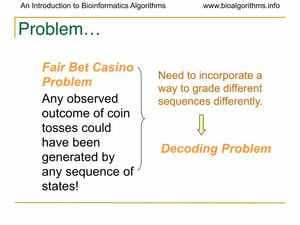
Problem…
Fair Bet Casino ProblemAny observed outcome of coin tosses could have been generated by any sequence of states!
Need to incorporate a way to grade different sequences differently.
Decoding Problem

An Introduction to Bioinformatics Algorithms www.bioalgorithms.info
P(x|fair coin) vs. P(x|biased coin)
• Suppose first that dealer never changes coins. Some definitions:• P(x|fair coin): prob. of the dealer using
the F coin and generating the outcome x.• P(x|biased coin): prob. of the dealer using
the B coin and generating outcome x.
An Introduction to Bioinformatics Algorithms www.bioalgorithms.info
P(x|fair coin) vs. P(x|biased coin)
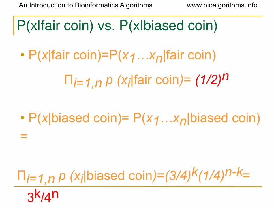
• P(x|fair coin)=P(x1…xn|fair coin)
Πi=1,n p (xi|fair coin)= (1/2)n
• P(x|biased coin)= P(x1…xn|biased coin)
=
Πi=1,n p (xi|biased coin)=(3/4)k(1/4)n-k=
3k/4n
• k - the number of Heads in x.

An Introduction to Bioinformatics Algorithms www.bioalgorithms.info
P(x|fair coin) vs. P(x|biased coin)
• P(x|fair coin) = P(x|biased coin)
• 1/2n = 3k/4n
• 2n = 3k
• n = k log23
• when k = n / log23 (k ~ 0.67n)
An Introduction to Bioinformatics Algorithms www.bioalgorithms.info
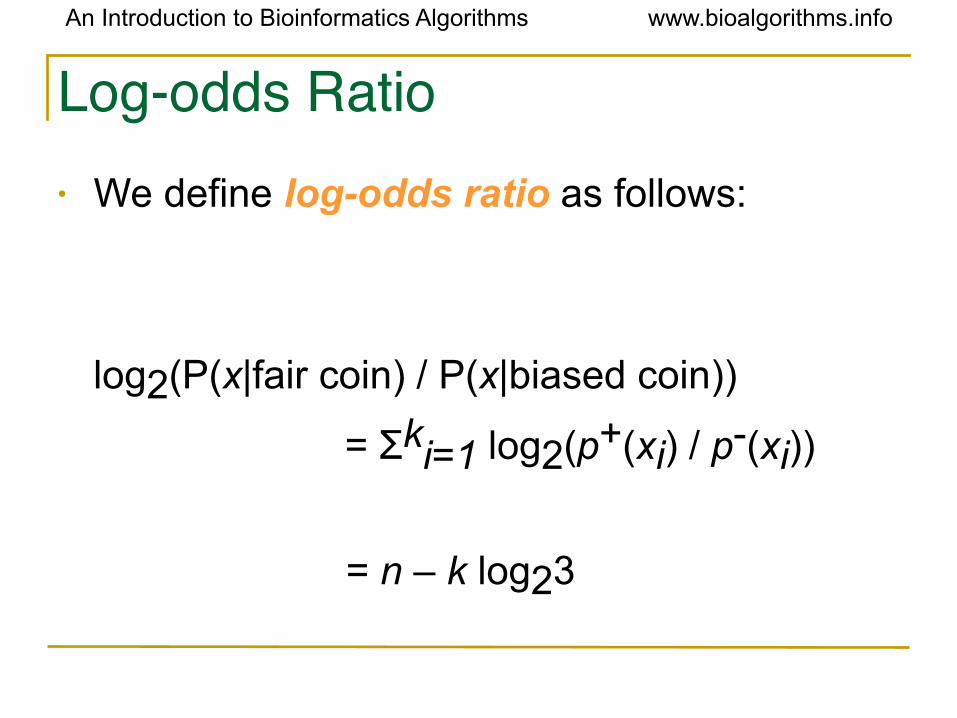
Log-odds Ratio• We define log-odds ratio as follows:
log2(P(x|fair coin) / P(x|biased coin))
= Σki=1 log2(p+(xi) / p-(xi))
= n – k log23

An Introduction to Bioinformatics Algorithms www.bioalgorithms.info
Computing Log-odds Ratio in Sliding Windows
x1x2x3x4x5x6x7x8…xn
Consider a sliding window of the outcome sequence. Find the log-odds for this short window.
Log-odds value
0
Fair coin most likely used
Biased coin most likely used
Disadvantages:- the length of CG-island is not known in advance- different windows may classify the same position differently

An Introduction to Bioinformatics Algorithms www.bioalgorithms.info
Hidden Markov Model (HMM)• Can be viewed as an abstract machine with k hidden states that emits symbols from an alphabet Σ.• Each state has its own probability distribution, and the machine switches between states according to this probability distribution.• While in a certain state, the machine makes 2 decisions:• What state should I move to next?• What symbol - from the alphabet Σ - should I emit?

An Introduction to Bioinformatics Algorithms www.bioalgorithms.info
Why “Hidden”?• Observers can see the emitted symbols of an
HMM but have no ability to know which state the HMM is currently in.
• Thus, the goal is to infer the most likely hidden states of an HMM based on the given sequence of emitted symbols.

An Introduction to Bioinformatics Algorithms www.bioalgorithms.info
HMM ParametersΣ: set of emission characters.
Ex.: Σ = {H, T} for coin tossing
Σ = {1, 2, 3, 4, 5, 6} for dice tossing
Q: set of hidden states, each emitting symbols from Σ.
Q={F,B} for coin tossing
An Introduction to Bioinformatics Algorithms www.bioalgorithms.info
HMM Parameters (cont’d)
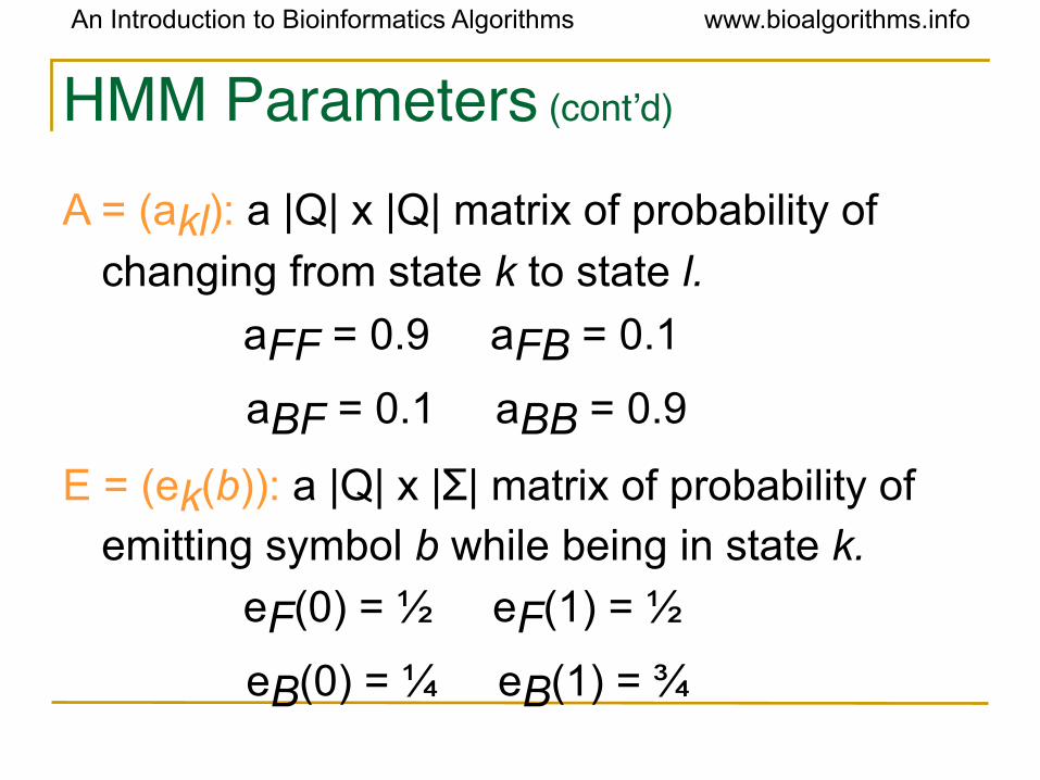
A = (akl): a |Q| x |Q| matrix of probability of
changing from state k to state l.
aFF = 0.9 aFB = 0.1
aBF = 0.1 aBB = 0.9
E = (ek(b)): a |Q| x |Σ| matrix of probability of emitting symbol b while being in state k.
eF(0) = ½ eF(1) = ½
eB(0) = ¼ eB(1) = ¾
An Introduction to Bioinformatics Algorithms www.bioalgorithms.info
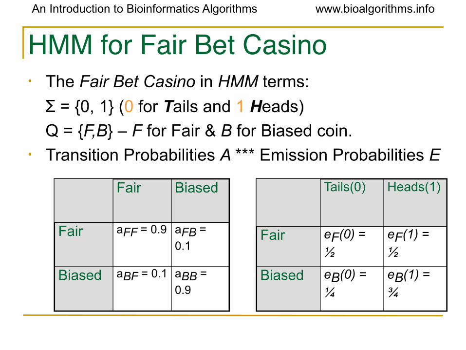
HMM for Fair Bet Casino• The Fair Bet Casino in HMM terms:
Σ = {0, 1} (0 for Tails and 1 Heads)
Q = {F,B} – F for Fair & B for Biased coin.• Transition Probabilities A *** Emission Probabilities E
Fair Biased
Fair aFF = 0.9 aFB =
0.1
Biased aBF = 0.1 aBB =
0.9
Tails(0) Heads(1)
Fair eF(0) = ½
eF(1) = ½
Biased eB(0) = ¼
eB(1) = ¾

An Introduction to Bioinformatics Algorithms www.bioalgorithms.info
HMM for Fair Bet Casino (cont’d)
HMM model for the Fair Bet Casino Problem

An Introduction to Bioinformatics Algorithms www.bioalgorithms.info
Hidden Paths• A path π = π1… πn in the HMM is defined as a
sequence of states.• Consider path π = FFFBBBBBFFF and sequence x =
01011101001
x 0 1 0 1 1 1 0 1 0 0 1
π = F F F B B B B B F F FP(xi|πi) ½ ½ ½ ¾ ¾ ¾ ¼ ¾ ½ ½ ½
P(πi-1 à πi) ½ 9/10 9/10 1/10 9/10 9/10 9/10 9/10 1/10 9/10 9/10
Transition probability from state πi-1 to state πi
Probability that xi was emitted from state πi

An Introduction to Bioinformatics Algorithms www.bioalgorithms.info
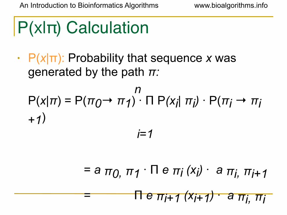
P(x|π) Calculation• P(x|π): Probability that sequence x was
generated by the path π: n P(x|π) = P(π0→ π1) · Π P(xi| πi) · P(πi → πi+1)
i=1
= a π0, π1 · Π e πi (xi) · a πi, πi+1
An Introduction to Bioinformatics Algorithms www.bioalgorithms.info
P(x|π) Calculation• P(x|π): Probability that sequence x was
generated by the path π: n P(x|π) = P(π0→ π1) · Π P(xi| πi) · P(πi → πi+1)
i=1
= a π0, π1 · Π e πi (xi) · a πi, πi+1
= Π e πi+1 (xi+1) · a πi, πi
+1
if we count from i=0
instead of i=1
An Introduction to Bioinformatics Algorithms www.bioalgorithms.info
Decoding Problem• Goal: Find an optimal hidden path of states
given observations.
• Input: Sequence of observations x = x1…xn
generated by an HMM M(Σ, Q, A, E)
• Output: A path that maximizes P(x|π) over all possible paths π.

An Introduction to Bioinformatics Algorithms www.bioalgorithms.info
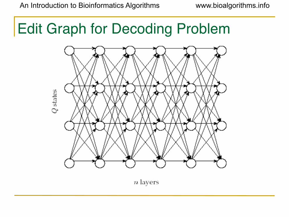
Building Manhattan for Decoding Problem
• Andrew Viterbi used the Manhattan grid model to solve the Decoding Problem.
• Every choice of π = π1… πn corresponds to
a path in the graph.
• The only valid direction in the graph is eastward.
• This graph has |Q|2(n-1) edges.
An Introduction to Bioinformatics Algorithms www.bioalgorithms.info
Edit Graph for Decoding Problem
An Introduction to Bioinformatics Algorithms www.bioalgorithms.info
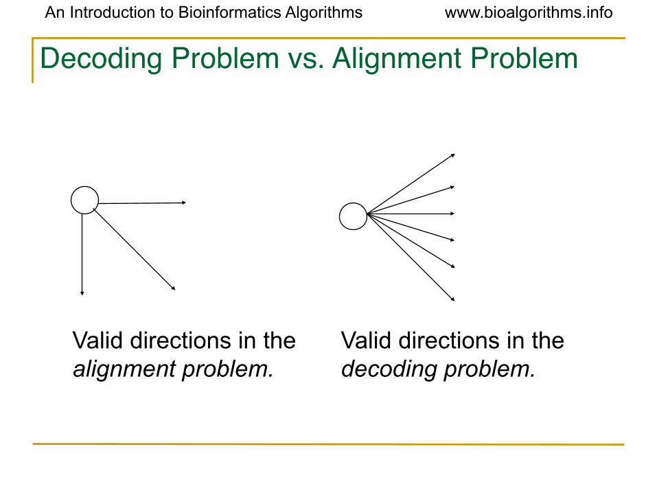
Decoding Problem vs. Alignment Problem
Valid directions in the alignment problem.
Valid directions in the decoding problem.
An Introduction to Bioinformatics Algorithms www.bioalgorithms.info
Decoding Problem as Finding a Longest Path in a DAG• The Decoding Problem is reduced to finding a longest path in the directed acyclic graph (DAG) above.
• Notes: the length of the path is defined as the product of its edges’ weights, not the sum.

An Introduction to Bioinformatics Algorithms www.bioalgorithms.info
Decoding Problem (cont’d)
• Every path in the graph has the probability P(x|π).
• The Viterbi algorithm finds the path that maximizes P(x|π) among all possible paths.
• The Viterbi algorithm runs in O(n|Q|2) time.
An Introduction to Bioinformatics Algorithms www.bioalgorithms.info
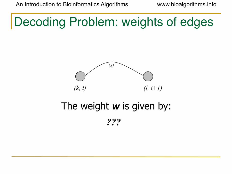
Decoding Problem: weights of edges
w
The weight w is given by:
???
(k, i) (l, i+1)

An Introduction to Bioinformatics Algorithms www.bioalgorithms.info
Decoding Problem: weights of edges
w
The weight w is given by:
??
(k, i) (l, i+1)
n P(x|π) = Π e πi+1 (xi+1) . a πi, πi+1
i=0
An Introduction to Bioinformatics Algorithms www.bioalgorithms.info
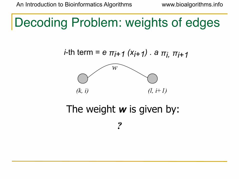
Decoding Problem: weights of edges
w
The weight w is given by:
?
(k, i) (l, i+1)
i-th term = e πi+1 (xi+1) . a πi, πi+1
An Introduction to Bioinformatics Algorithms www.bioalgorithms.info
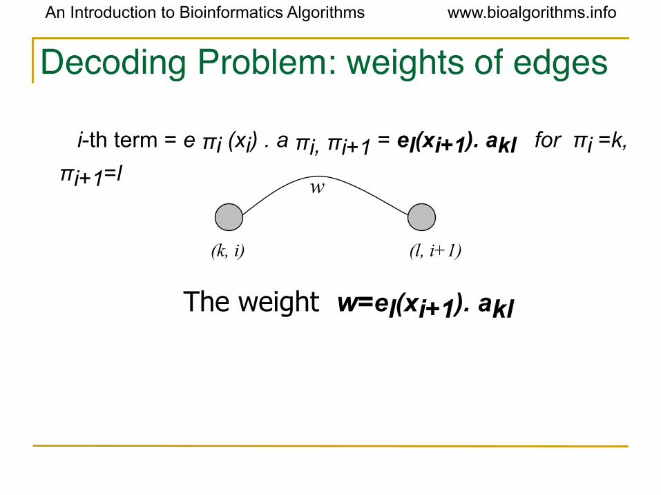
Decoding Problem: weights of edges
w
The weight w=el(xi+1). akl
(k, i) (l, i+1)
i-th term = e πi (xi) . a πi, πi+1 = el(xi+1). akl for πi =k,
πi+1=l

An Introduction to Bioinformatics Algorithms www.bioalgorithms.info
Decoding Problem and Dynamic Programming
sl,i+1 = maxk Є Q {sk,i · weight of edge between (k,i) and (l,i
+1)}=
maxk Є Q {sk,i · akl · el (xi+1)
}=
el (xi+1) · maxk Є Q {sk,i · akl}

An Introduction to Bioinformatics Algorithms www.bioalgorithms.info
Decoding Problem (cont’d)
• Initialization:• sbegin,0 = 1
• sk,0 = 0 for k ≠ begin.
• Let π* be the optimal path. Then,
P(x|π*) = maxk Є Q {sk,n . ak,end}

An Introduction to Bioinformatics Algorithms www.bioalgorithms.info
Viterbi Algorithm• The value of the product can become
extremely small, which leads to overflowing.• To avoid overflowing, use log value instead.
sk,i+1= logel(xi+1) + max k Є Q {sk,i + log(akl)}
An Introduction to Bioinformatics Algorithms www.bioalgorithms.info
Forward-Backward Problem
Given: a sequence of coin tosses generated by an HMM.
Goal: find the probability that the dealer was using a biased coin at a particular time.
An Introduction to Bioinformatics Algorithms www.bioalgorithms.info
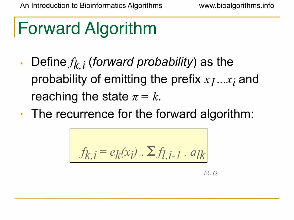
Forward Algorithm
• Define fk,i (forward probability) as the
probability of emitting the prefix x1…xi and
reaching the state π = k.• The recurrence for the forward algorithm:
fk,i = ek(xi) . Σ fl,i-1 . alk l Є Q
An Introduction to Bioinformatics Algorithms www.bioalgorithms.info
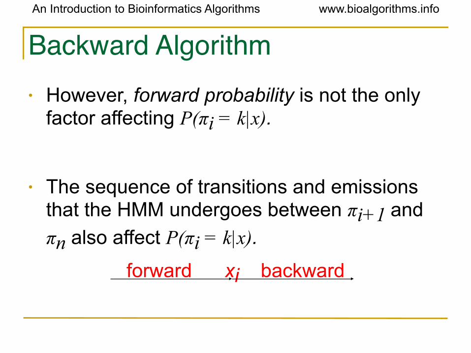
Backward Algorithm• However, forward probability is not the only
factor affecting P(πi = k|x).
• The sequence of transitions and emissions that the HMM undergoes between πi+1 and
πn also affect P(πi = k|x).
forward xi backward
An Introduction to Bioinformatics Algorithms www.bioalgorithms.info
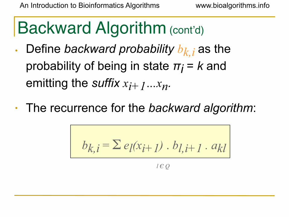
Backward Algorithm (cont’d)
• Define backward probability bk,i as the
probability of being in state πi = k and
emitting the suffix xi+1…xn.
• The recurrence for the backward algorithm:
bk,i = Σ el(xi+1) . bl,i+1 . akl l Є Q
An Introduction to Bioinformatics Algorithms www.bioalgorithms.info
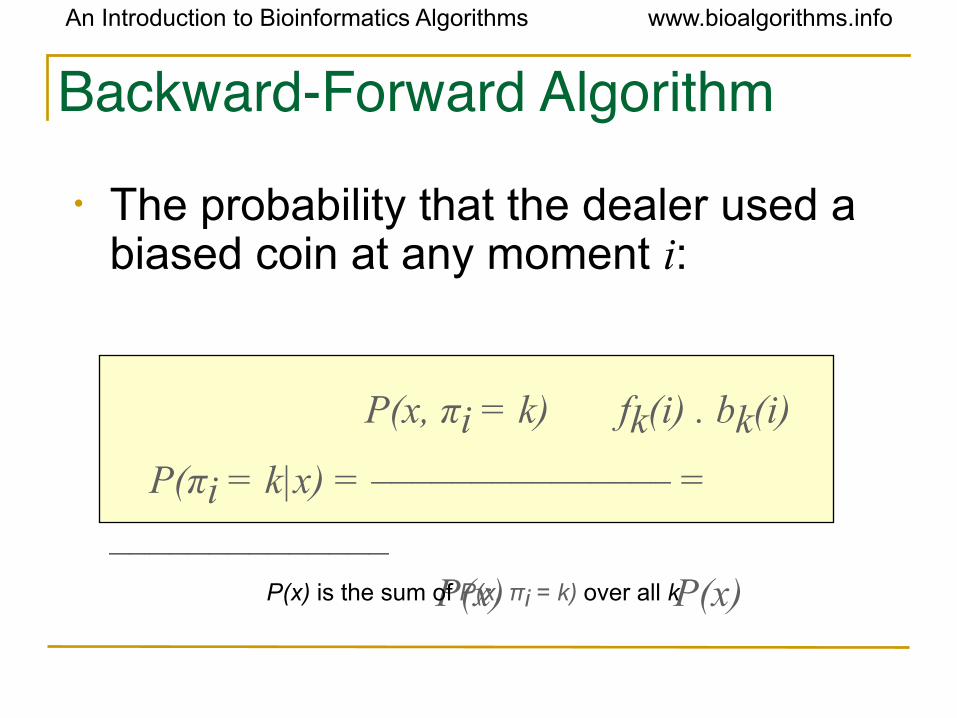
Backward-Forward Algorithm
• The probability that the dealer used a biased coin at any moment i:
P(x, πi = k) fk(i) . bk(i)
P(πi = k|x) = _______________ = ______________
P(x) P(x) P(x) is the sum of P(x, πi = k) over all k

An Introduction to Bioinformatics Algorithms www.bioalgorithms.info
Finding Distant Members of a Protein Family
• A distant cousin of functionally related sequences in a protein family may have weak pairwise similarities with each member of the family and thus fail significance test.
• However, they may have weak similarities with many members of the family.
• The goal is to align a sequence to all members of the family at once.
• Family of related proteins can be represented by their multiple alignment and the corresponding profile.
An Introduction to Bioinformatics Algorithms www.bioalgorithms.info
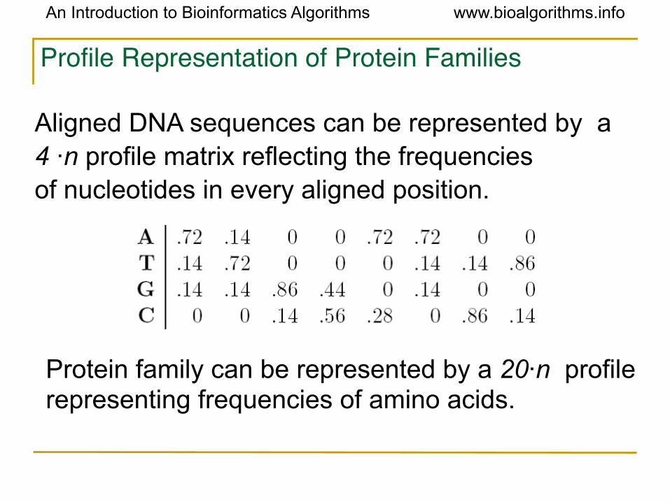
Profile Representation of Protein Families
Aligned DNA sequences can be represented by a 4 ·n profile matrix reflecting the frequencies of nucleotides in every aligned position.
Protein family can be represented by a 20·n profile representing frequencies of amino acids.
An Introduction to Bioinformatics Algorithms www.bioalgorithms.info
Profiles and HMMs
• HMMs can also be used for aligning a sequence against a profile representing
protein family.• A 20·n profile P corresponds to n
sequentially linked match states M1,…,Mn in the profile HMM of P.
An Introduction to Bioinformatics Algorithms www.bioalgorithms.info
Multiple Alignments and Protein Family Classification
• Multiple alignment of a protein family shows variations in conservation along the length of a protein
• Example: after aligning many globin proteins, the biologists recognized that the helices region in globins are more conserved than others.
An Introduction to Bioinformatics Algorithms www.bioalgorithms.info
What are Profile HMMs ?
• A Profile HMM is a probabilistic representation of a multiple alignment.
• A given multiple alignment (of a protein family) is used to build a profile HMM.
• This model then may be used to find and score less obvious potential matches of new protein sequences.

An Introduction to Bioinformatics Algorithms www.bioalgorithms.info
Profile HMM
A profile HMM
An Introduction to Bioinformatics Algorithms www.bioalgorithms.info
Building a profile HMM
• Multiple alignment is used to construct the HMM model.• Assign each column to a Match state in HMM. Add Insertion and
Deletion state. • Estimate the emission probabilities according to amino acid
counts in column. Different positions in the protein will have different emission probabilities.
• Estimate the transition probabilities between Match, Deletion and Insertion states
• The HMM model gets trained to derive the optimal parameters.
An Introduction to Bioinformatics Algorithms www.bioalgorithms.info
States of Profile HMM
• Match states M1…Mn (plus begin/end states)
• Insertion states I0I1…In
• Deletion states D1…Dn

An Introduction to Bioinformatics Algorithms www.bioalgorithms.info
Transition Probabilities in Profile HMM
• log(aMI)+log(aIM) = gap initiation penalty
• log(aII) = gap extension penalty

An Introduction to Bioinformatics Algorithms www.bioalgorithms.info
Emission Probabilities in Profile HMM• Probabilty of emitting a symbol a at an insertion state Ij:
eIj(a) = p(a)
where p(a) is the frequency of the occurrence of the symbol a in all the sequences.

An Introduction to Bioinformatics Algorithms www.bioalgorithms.info
Profile HMM Alignment
• Define vMj (i) as the logarithmic likelihood
score of the best path for matching x1..xi to
profile HMM ending with xi emitted by the
state Mj.
• vIj (i) and vDj (i) are defined similarly.
An Introduction to Bioinformatics Algorithms www.bioalgorithms.info
Profile HMM Alignment: Dynamic Programming
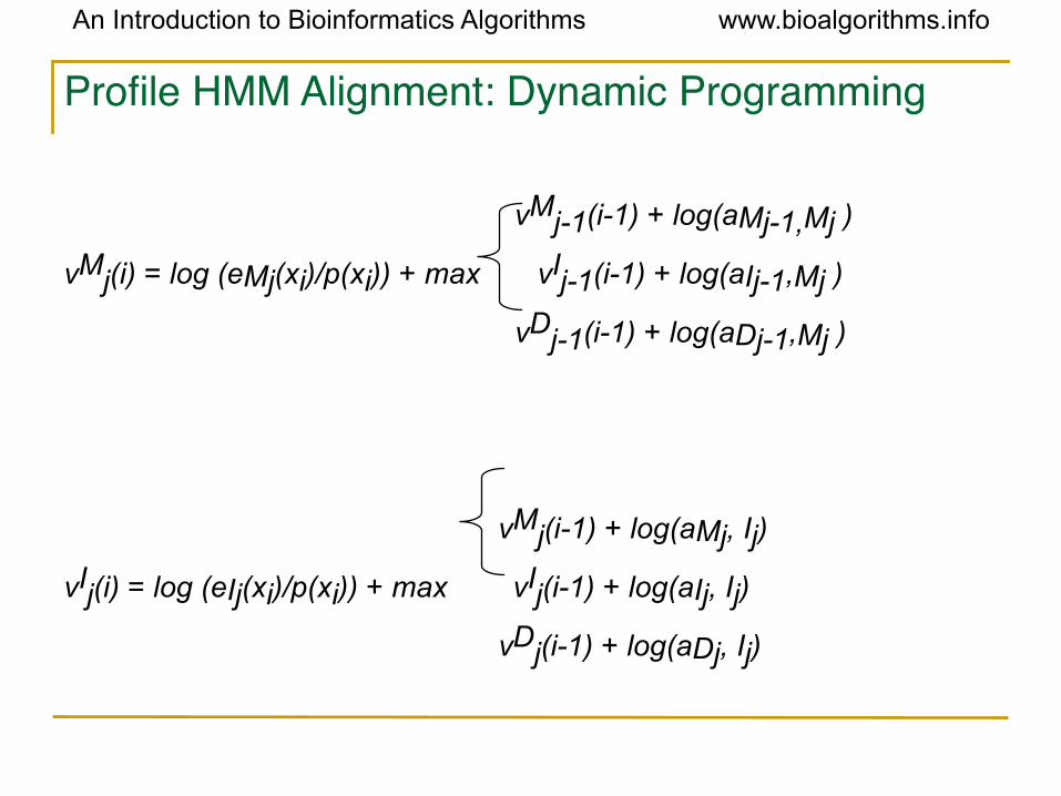
vMj-1(i-1) + log(aMj-1,Mj )
vMj(i) = log (eMj(xi)/p(xi)) + max vIj-1(i-1) + log(aIj-1,Mj )
vDj-1(i-1) + log(aDj-1,Mj )
vMj(i-1) + log(aMj, Ij)
vIj(i) = log (eIj(xi)/p(xi)) + max vIj(i-1) + log(aIj, Ij)
vDj(i-1) + log(aDj, Ij)
An Introduction to Bioinformatics Algorithms www.bioalgorithms.info
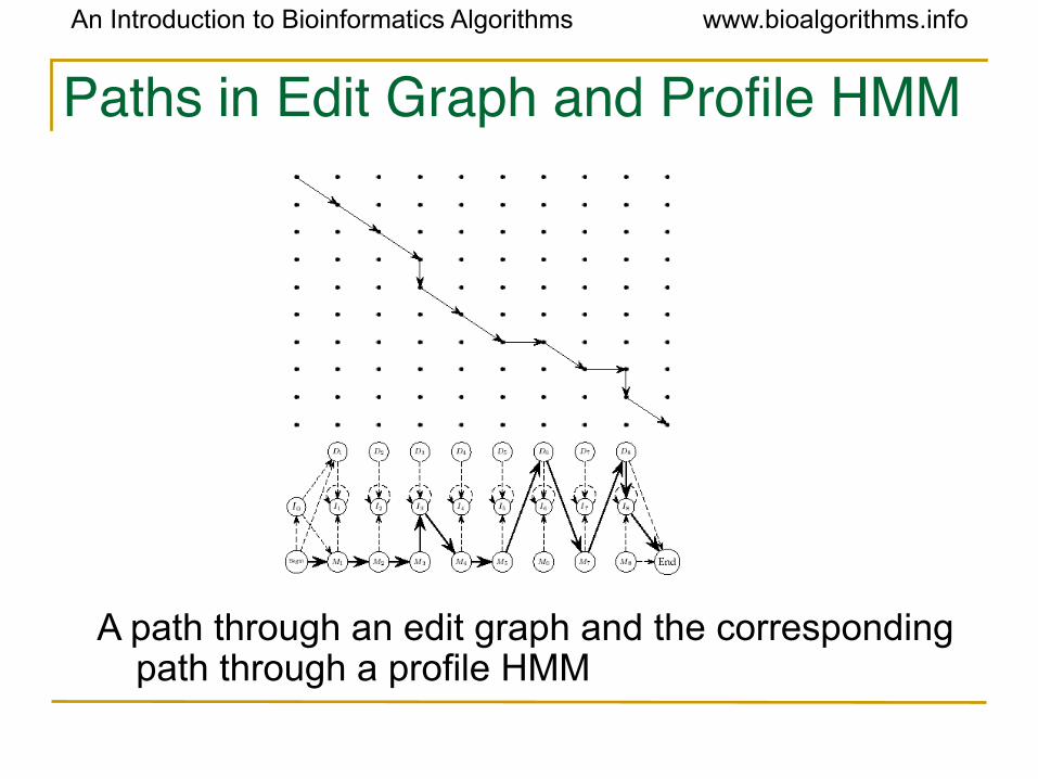
Paths in Edit Graph and Profile HMM
A path through an edit graph and the corresponding path through a profile HMM
An Introduction to Bioinformatics Algorithms www.bioalgorithms.info
Making a Collection of HMM for Protein Families
• Use Blast to separate a protein database into families of related proteins
• Construct a multiple alignment for each protein family.• Construct a profile HMM model and optimize the
parameters of the model (transition and emission probabilities).
• Align the target sequence against each HMM to find the best fit between a target sequence and an HMM
An Introduction to Bioinformatics Algorithms www.bioalgorithms.info
Application of Profile HMM to Modeling Globin Proteins• Globins represent a large collection of protein
sequences • 400 globin sequences were randomly selected
from all globins and used to construct a multiple alignment.
• Multiple alignment was used to assign an initial HMM
• This model then get trained repeatedly with model lengths chosen randomly between 145 to 170, to get an HMM model optimized probabilities.
An Introduction to Bioinformatics Algorithms www.bioalgorithms.info
How Good is the Globin HMM?• 625 remaining globin sequences in the database were
aligned to the constructed HMM resulting in a multiple alignment. This multiple alignment agrees extremely well with the structurally derived alignment.
• 25,044 proteins, were randomly chosen from the database and compared against the globin HMM.
• This experiment resulted in an excellent separation between globin and non-globin families.

An Introduction to Bioinformatics Algorithms www.bioalgorithms.info
PFAM• Pfam decribes protein domains • Each protein domain family in Pfam has:
- Seed alignment: manually verified multiple alignment of a representative set of sequences.
- HMM built from the seed alignment for further database searches.
- Full alignment generated automatically from the HMM• The distinction between seed and full alignments facilitates Pfam
updates.- Seed alignments are stable resources.- HMM profiles and full alignments can be updated with
newly found amino acid sequences.

An Introduction to Bioinformatics Algorithms www.bioalgorithms.info
PFAM Uses• Pfam HMMs span entire domains that include
both well-conserved motifs and less-conserved regions with insertions and deletions.
• It results in modeling complete domains that facilitates better sequence annotation and leeds to a more sensitive detection.
An Introduction to Bioinformatics Algorithms www.bioalgorithms.info
HMM Parameter Estimation• So far, we have assumed that the transition
and emission probabilities are known.
• However, in most HMM applications, the probabilities are not known. It’s very hard to estimate the probabilities.
An Introduction to Bioinformatics Algorithms www.bioalgorithms.info
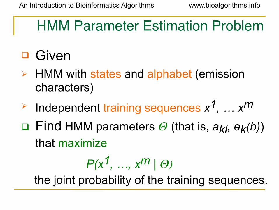
HMM Parameter Estimation Problem
Given HMM with states and alphabet (emission
characters)
Independent training sequences x1, … xm
Find HMM parameters Θ (that is, akl, ek(b))
that maximize
P(x1, …, xm | Θ) the joint probability of the training sequences.
An Introduction to Bioinformatics Algorithms www.bioalgorithms.info
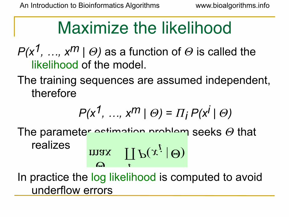
Maximize the likelihoodP(x1, …, xm | Θ) as a function of Θ is called the
likelihood of the model.The training sequences are assumed independent,
therefore
P(x1, …, xm | Θ) = Πi P(xi | Θ)
The parameter estimation problem seeks Θ that realizes
In practice the log likelihood is computed to avoid underflow errors

An Introduction to Bioinformatics Algorithms www.bioalgorithms.info
Two situationsKnown paths for training sequences
CpG islands marked on training sequences
One evening the casino dealer allows us to see when he changes dice
Unknown paths
CpG islands are not marked
Do not see when the casino dealer changes dice
An Introduction to Bioinformatics Algorithms www.bioalgorithms.info
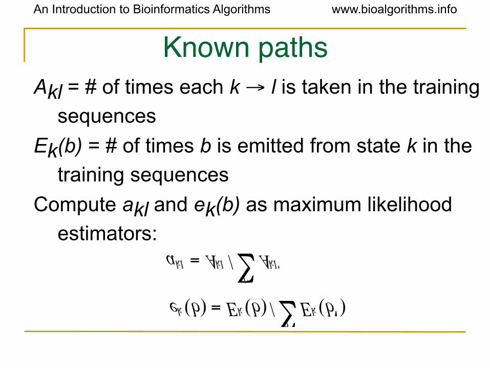
Known pathsAkl = # of times each k → l is taken in the training
sequences
Ek(b) = # of times b is emitted from state k in the
training sequences
Compute akl and ek(b) as maximum likelihood
estimators:

An Introduction to Bioinformatics Algorithms www.bioalgorithms.info
Pseudocounts Some state k may not appear in any of the training
sequences. This means Akl = 0 for every state l
and akl cannot be computed with the given
equation. To avoid this overfitting use predetermined
pseudocounts rkl and rk(b).
Akl = # of transitions k→l + rkl
Ek(b) = # of emissions of b from k + rk(b)
The pseudocounts reflect our prior biases about the probability values.

An Introduction to Bioinformatics Algorithms www.bioalgorithms.info
Unknown paths: Viterbi trainingIdea: use Viterbi decoding to compute the most
probable path for training sequence xStart with some guess for initial parameters and compute π* the most probable path for x using initial parameters.Iterate until no change in π* :
4. Determine Akl and Ek(b) as before5. Compute new parameters akl and ek(b) using the
same formulas as before6. Compute new π* for x and the current parameters

An Introduction to Bioinformatics Algorithms www.bioalgorithms.info
Viterbi training analysis The algorithm converges precisely
There are finitely many possible paths.New parameters are uniquely determined by the current π*.There may be several paths for x with the same probability, hence must compare the new π* with all previous paths having highest probability.
Does not maximize the likelihood Πx P(x | Θ) but the contribution to the likelihood of the most probable path Πx P
(x | Θ, π*) In general performs less well than Baum-Welch

An Introduction to Bioinformatics Algorithms www.bioalgorithms.info
Unknown paths: Baum-Welch
Idea:2. Guess initial values for parameters.
art and experience, not science4. Estimate new (better) values for parameters.
how ?6. Repeat until stopping criteria is met.
what criteria ?

An Introduction to Bioinformatics Algorithms www.bioalgorithms.info
Better values for parameters
Would need the Akl and Ek(b) values but cannot
count (the path is unknown) and do not want to use a most probable path.
For all states k,l, symbol b and training sequence x
Compute Akl and Ek(b) as expected
values, given the current parameters
An Introduction to Bioinformatics Algorithms www.bioalgorithms.info
NotationFor any sequence of characters x emitted
along some unknown path π, denote by πi = k the assumption that the state
at position i (in which xi is emitted) is k.
An Introduction to Bioinformatics Algorithms www.bioalgorithms.info
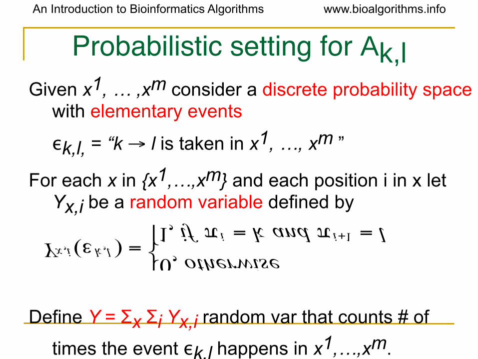
Probabilistic setting for Ak,lGiven x1, … ,xm consider a discrete probability space
with elementary events
εk,l, = “k → l is taken in x1, …, xm ”
For each x in {x1,…,xm} and each position i in x let Yx,i be a random variable defined by
Define Y = Σx Σi Yx,i random var that counts # of
times the event εk,l happens in x1,…,xm.
An Introduction to Bioinformatics Algorithms www.bioalgorithms.info
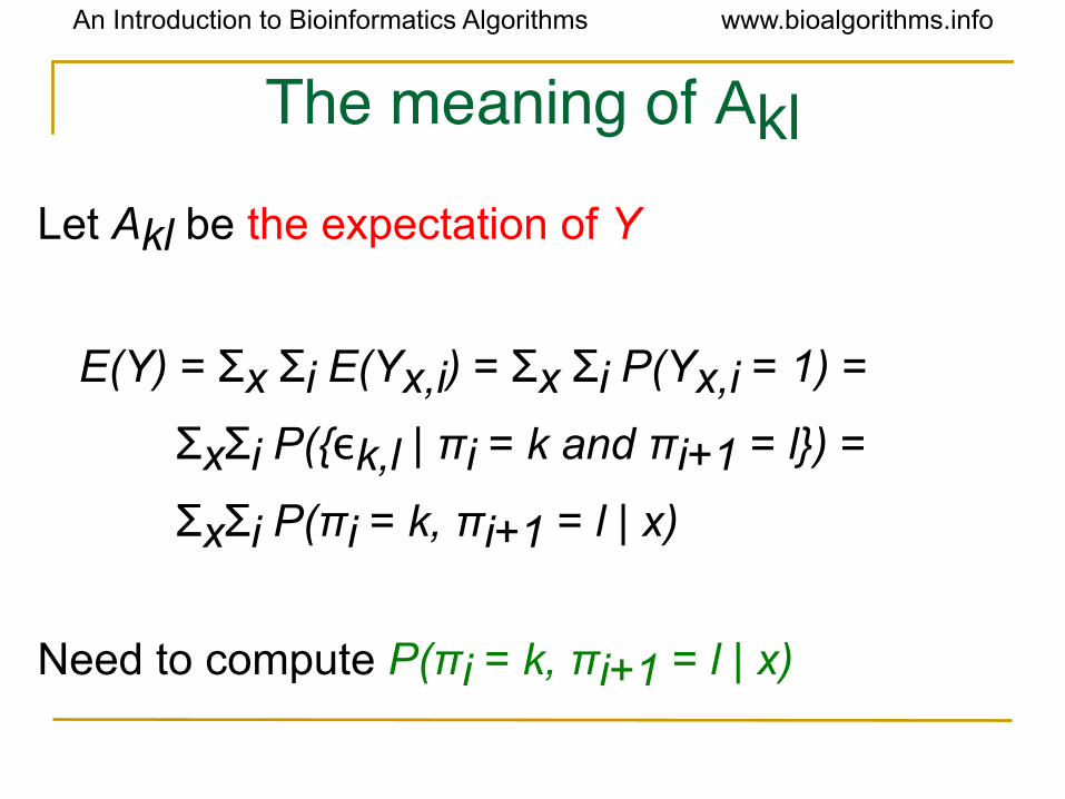
The meaning of Akl
Let Akl be the expectation of Y
E(Y) = Σx Σi E(Yx,i) = Σx Σi P(Yx,i = 1) =
ΣxΣi P({εk,l | πi = k and πi+1 = l}) =
ΣxΣi P(πi = k, πi+1 = l | x)
Need to compute P(πi = k, πi+1 = l | x)

An Introduction to Bioinformatics Algorithms www.bioalgorithms.info
Probabilistic setting for Ek(b)
Given x1, … ,xm consider a discrete probability space with elementary events
εk,b = “b is emitted in state k in x1, … ,xm ”
For each x in {x1,…,xm} and each position i in x let Yx,i be a random variable defined by
Define Y = Σx Σi Yx,i random var that counts # of
times the event εk,b happens in x1,…,xm.

An Introduction to Bioinformatics Algorithms www.bioalgorithms.info
The meaning of Ek(b)
Let Ek(b) be the expectation of Y
E(Y) = Σx Σi E(Yx,i) = Σx Σi P(Yx,i = 1) =
ΣxΣi P({εk,b | xi = b and πi = k})
Need to compute P(πi = k | x)

An Introduction to Bioinformatics Algorithms www.bioalgorithms.info
Computing new parametersConsider x = x1…xn training sequence
Concentrate on positions i and i+1
Use the forward-backward values:
fki = P(x1 … xi , πi = k)
bki = P(xi+1 … xn | πi = k)
An Introduction to Bioinformatics Algorithms www.bioalgorithms.info
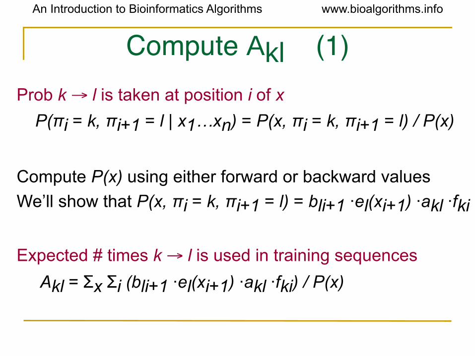
Compute Akl (1)Prob k → l is taken at position i of x
P(πi = k, πi+1 = l | x1…xn) = P(x, πi = k, πi+1 = l) / P(x)
Compute P(x) using either forward or backward values
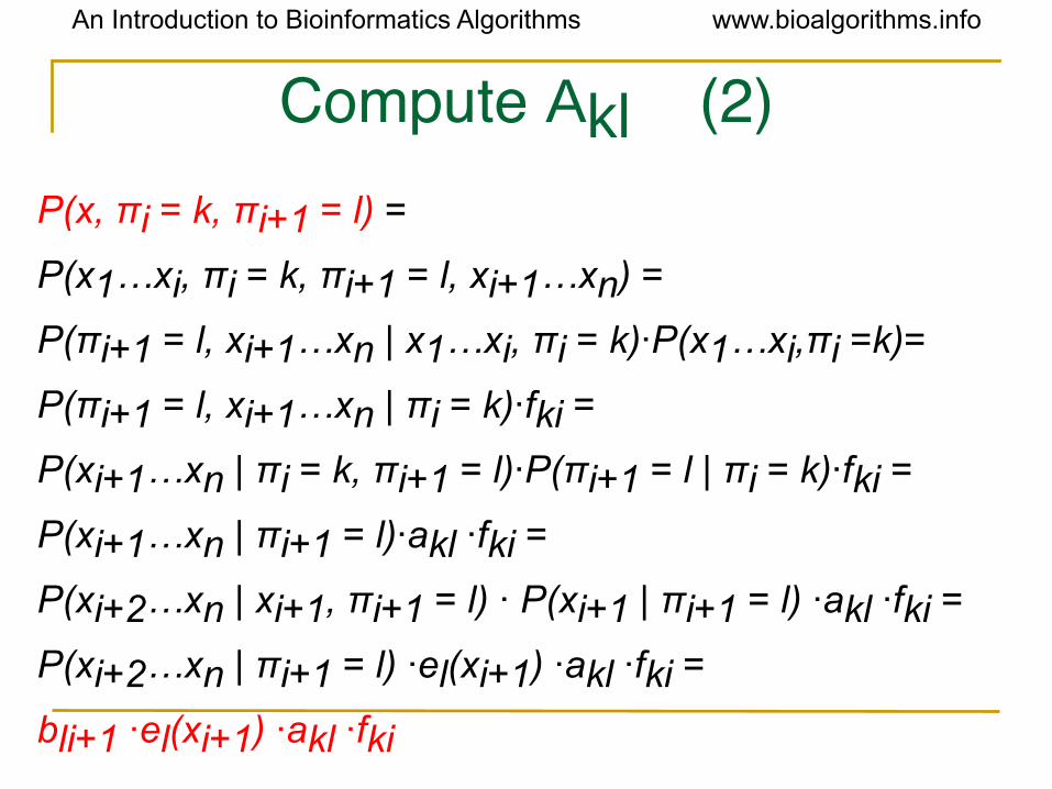
We’ll show that P(x, πi = k, πi+1 = l) = bli+1 ·el(xi+1) ·akl ·fki
Expected # times k → l is used in training sequences
Akl = Σx Σi (bli+1 ·el(xi+1) ·akl ·fki) / P(x)
An Introduction to Bioinformatics Algorithms www.bioalgorithms.info
Compute Akl (2)P(x, πi = k, πi+1 = l) =
P(x1…xi, πi = k, πi+1 = l, xi+1…xn) =
P(πi+1 = l, xi+1…xn | x1…xi, πi = k)·P(x1…xi,πi =k)=
P(πi+1 = l, xi+1…xn | πi = k)·fki =
P(xi+1…xn | πi = k, πi+1 = l)·P(πi+1 = l | πi = k)·fki =
P(xi+1…xn | πi+1 = l)·akl ·fki =
P(xi+2…xn | xi+1, πi+1 = l) · P(xi+1 | πi+1 = l) ·akl ·fki =
P(xi+2…xn | πi+1 = l) ·el(xi+1) ·akl ·fki =
bli+1 ·el(xi+1) ·akl ·fki

An Introduction to Bioinformatics Algorithms www.bioalgorithms.info
Compute Ek(b)
Prob xi of x is emitted in state k
P(πi = k | x1…xn) = P(πi = k, x1…xn)/P(x)
P(πi = k, x1…xn) = P(x1…xi,πi = k,xi+1…xn) =
P(xi+1…xn | x1…xi,πi = k) · P(x1…xi,πi = k) =
P(xi+1…xn | πi = k) · fki = bki · fkiExpected # times b is emitted in state k

An Introduction to Bioinformatics Algorithms www.bioalgorithms.info
Finally, new parameters
Can add pseudocounts as before.
An Introduction to Bioinformatics Algorithms www.bioalgorithms.info
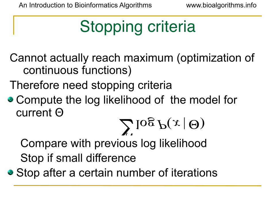
Stopping criteria
Cannot actually reach maximum (optimization of continuous functions)
Therefore need stopping criteriaCompute the log likelihood of the model for current Θ
Compare with previous log likelihoodStop if small difference
Stop after a certain number of iterations
An Introduction to Bioinformatics Algorithms www.bioalgorithms.info
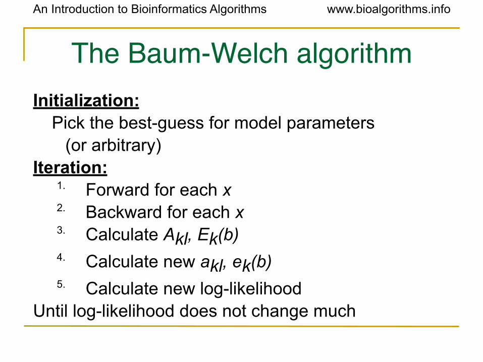
The Baum-Welch algorithmInitialization:
Pick the best-guess for model parameters(or arbitrary)
Iteration:1. Forward for each x2. Backward for each x3. Calculate Akl, Ek(b)4. Calculate new akl, ek(b)5. Calculate new log-likelihood
Until log-likelihood does not change much

An Introduction to Bioinformatics Algorithms www.bioalgorithms.info
Baum-Welch analysis
Log-likelihood is increased by iterations
Baum-Welch is a particular case of the EM (expectation maximization) algorithm
Convergence to local maximum. Choice of initial parameters determines local maximum to which the algorithm converges

An Introduction to Bioinformatics Algorithms www.bioalgorithms.info
Speech Recognition• Create an HMM of the words in a language
• Each word is a hidden state in Q.• Each of the basic sounds in the language is
a symbol in Σ.
• Input: use speech as the input sequence.• Goal: find the most probable sequence of
states.
An Introduction to Bioinformatics Algorithms www.bioalgorithms.info
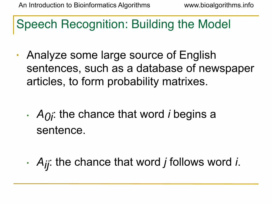
Speech Recognition: Building the Model
• Analyze some large source of English sentences, such as a database of newspaper articles, to form probability matrixes.
• A0i: the chance that word i begins a
sentence.
• Aij: the chance that word j follows word i.
An Introduction to Bioinformatics Algorithms www.bioalgorithms.info
Building the Model (cont’d)
• Analyze English speakers to determine what sounds are emitted with what words.
• Ek(b): the chance that sound b is spoken in
word k. Allows for alternate pronunciation of words.
An Introduction to Bioinformatics Algorithms www.bioalgorithms.info
Speech Recognition: Using the Model
• Use the same dynamic programming algorithm as before• Weave the spoken sounds through the
model the same way we wove the rolls of the die through the casino model.
• π represents the most likely set of words.
An Introduction to Bioinformatics Algorithms www.bioalgorithms.info
Using the Model (cont’d)
• How well does it work?• Common words, such as ‘the’, ‘a’, ‘of’ make
prediction less accurate, since there are so many words that follow normally.
An Introduction to Bioinformatics Algorithms www.bioalgorithms.info
Improving Speech Recognition• Initially, we were using a ‘bigram,’ a graph
connecting every two words.• Expand that to a ‘trigram’
• Each state represents two words spoken in succession.
• Each edge joins those two words (A B) to another state representing (B C)
• Requires n3 vertices and edges, where n is the number of words in the language.
• Much better, but still limited context.

An Introduction to Bioinformatics Algorithms www.bioalgorithms.info
References• Slides for CS 262 course at Stanford given by
Serafim Batzoglou


