Hidden Markov Models

State Space and Hidden Markov Models

Aliaksandr Hubin

Oslo 2014

Kunsch, H.R., State Space and Hidden Markov Models. ETH-Zurich, Zurich;

Contents

1. Introduction

2. Markov Chains

3. Hidden Markov and State Space Model

4. Filtering and Smoothing of State Densities

5. Estimation of Parameters

6. Spatial-Temporal Model

11/10/2014 ALIAKSANDR HUBIN. STK 9200 2

IntroductionHMM

Broadly speaking we will address the models where observations are noisy and incomplete functions of some underlying unobservable process, called the state process, which is assumed to have simple markovian dynamics.


Markov chains• Set of states:

• Process moves from one state to another generating a sequence of states :

• Markov chain property: probability of each subsequent state depends only on what was the previous state:

• To define Markov chain, the following probabilities have to be specified:

transition probabilities matrix and initial probabilities

• The output of the process is the set of states at each instant of time

• Joint probability of all states sequence:


,...2,1},,,,{ 21 immmx Ni ,,,, 21 kxxx

)|(),,,|( 1121 kkkk xxPxxxxP

)|( jiij mmPa )( ii mP

)()|()|()|(

),,,()|(

),,,(),,,|(),,,(

112211

1211

12112121

xPxxPxxPxxP

xxxPxxP

xxxPxxxxPxxxP

kkkk

kkk

kkkk

Simple Example of Markov Model

•Epigenetic state process is considered

•Two states : ‘Methylated’ and ‘Non-methylated’.

•Initial probabilities: P(‘Methylated’)=0.4 , P(‘Non-

methylated’)=0.6

•Transition probabilities described in the graph ->

•Inference example: Suppose we want to calculate a probability of a sequence of states in our example, {‘Methylated’,’ Methylated’,’ Non-methylated’, Non-methylated’}. This then corresponds to 0.4*0.3*0.7*0.8 = 6.72%


Hidden Markov Models• The observations are represented by a probabilistic function (discrete

or continuous) of a state instead of an one-to-one correspondence of a state

•The following components describe a Hidden Markov Model in the simplest case:

1. Distribution of transition probabilities ;

2. Distribution of initial state probabilities ;

3. Distribution of observation probabilities 𝜗𝑖 = 𝑃 𝑦𝑖 𝑥𝑖 .

𝑥𝑖 ∈ 𝑅𝑁- are usually addressed as state space models;

𝑥𝑖∈ {𝑚1, … ,𝑚𝑁} – are usually addressed as hidden markov chains;

Parameters listed above estimation might be very challenging for complicated models!


)|( jiij mmPa

)( ii mP

Hidden Markov ModelsThe following components describe a Hidden Markov Model in the general case:

1. Distribution of initial state probabilities 𝑋0~𝑎0 𝑥 𝑑𝜇(𝑥);

2. Distribution of transition probabilities 𝑋𝑡| 𝑋𝑡−1 = 𝑥𝑡−1 ~𝑎𝑡 𝑥𝑡−1, 𝑥 𝑑𝜇(𝑥);

3. Distribution of observation probabilities 𝑌𝑡 (𝑋𝑡= 𝑥𝑡 ~𝑏𝑡 𝑥𝑡 , 𝑦 𝑑𝑣 𝑦 ;

4. The joint density of the process and observations then looks as follows:

𝑃 𝑋0, … , 𝑋𝑇 , 𝑌1, … , 𝑌𝑇 = 𝑎0(𝑥0) 𝑡=1𝑇 𝑎𝑡 𝑥𝑡−1, 𝑥𝑡 𝑏𝑡(𝑥𝑡, 𝑦𝑡) .


Simple Example of HMM


•Whether state process is considered

•Two discrete states : ‘Methylated’ and ‘Non-methylated’.

•Initial probabilities: P(‘Methylated’)=0.4 , P(‘Non-

methylated’)=0.6

•Transition probabilities described in the graph ->

•Locations associated are observed with respect to their state-dependent probabilities

•Corresponding observation probabilities are represented in the graph ->

Graphical illustration of the Hidden Markov Model


Project application

Let further:

•𝐼𝑡 be a binary variable indication whether location t is methylated

•𝐸𝑡 be a binary varibale indicating whether the gene, to which location 𝑡 belongs is expressed

•𝑛𝑡 be an amount of reads for location t

•𝑦𝑡 be a binomial variable indicating the number of methylated reads at location t

•𝑧𝑡 be a quantitative measure of some phenotypic response for the expressed genes at location t


Project application


𝐸1 𝐸𝑡 𝐸𝑡+1 𝐸𝑇

𝐼𝑡+1 𝐼𝑇

𝑧1 𝑧𝑡 𝑧𝑡+1 𝑧𝑇

𝑦1 𝑦𝑡 𝑦𝑡+1 𝑦𝑇

……

…

…

……

…

…

𝐼1 𝐼𝑡 Initial

Extended

Project application

•𝐼𝑡 = 1, − location 𝑡 is methylated0,− location 𝑡 is not methylated

~ 𝑃(𝐼𝑡) = 𝑃1, − location 𝑡 is methylated𝑃2, −location 𝑡 is not methylated

•𝑃𝑖𝑗 = 𝑃 𝐼𝑡 = 𝑗 𝐼𝑡−1 = 𝑖 −define dynamic structures in the given neighborhood

•𝑦𝑡|𝐼𝑡, 𝑛𝑡 − number of metylated observations in given reads and methylation status

•𝑃(𝑦𝑡 𝐼𝑡 , 𝑛𝑡 = 𝑃𝐵𝑖𝑛𝑜𝑚 𝑛𝑡,𝑃 𝐼𝑡𝑦𝑡 − it has binomial distribution


Extensions of the model

Let 𝑝𝑡be continuous: define stochastic process 𝑝(𝐼𝑡)= 𝐵𝑒𝑡𝑎(𝛽

𝑝𝑡−1

1−𝑝𝑡−1)

𝐵𝑒𝑡𝑎(𝛽𝑞𝐼𝑡

1−𝑞𝐼𝑡)

, giving similarities when the state do

not change but a renewal in cases where the state changes.

Link state transition probabilities to underlying genomic structure

Look at more global structures than transition probabilities 𝑃𝑖𝑗:

-address more complex models describing more global structures (ARIMA, n-markov chains, etc.)

-use simple markov chain model above as a first step, but then extract more global features of {𝐼𝑡}

Consider more complex spatial structures than the one-directional approach above.

Simultaneous modelling of several tissues and/or individuals at the same time.


Parameters’ estimation & Inference1. Viterbi algorithm for fitting the joint distribution of the most probable sequence of states

𝑎𝑟𝑔𝑚𝑎𝑥𝑥1:𝑇{𝑃(𝑥1:𝑇|𝑑1:𝑇)}

2. Forward algorithm for fitting filtered probability of a given state, given data up to 𝑃(𝑥𝑡|𝑑1, … , 𝑑𝑡)

3. Forward–backward algorithm for fitting the smoothed probability of a given state, given all data 𝑃(𝑥𝑘|𝑑1, … , 𝑑𝑇)

4. Maximal likelihood maximization or Bayesian methods for parameters’ vector 𝜃 estimation

Where 𝑑𝑡 is data at point t;

Note that these algorithms are linear in the number of time points.


Inference. Filtering.1. Recursion in k for prediction density of the states:

𝑓𝑡+𝑘|𝑡 𝑥𝑡+𝑘 𝑦1𝑡 = 𝑎𝑡+𝑘 𝑥, 𝑥𝑡+𝑘 𝑓𝑡+𝑘−1|𝑡 𝑥 𝑦1

𝑡 𝑑𝜇(𝑥)

2. Prediction densities for the observations given the corresponding prediction densities of the states:

𝑝 𝑦𝑡+𝑘 𝑦1𝑡 = 𝑏𝑡+𝑘 𝑥, 𝑦𝑡+𝑘 𝑓𝑡+𝑘 𝑥 𝑦1

𝑡 𝑑𝜇(𝑥)

3. Thus, filtering densities of the states can be computed according to the following forward recursion in t (starting with 𝑓0|0):

𝑓𝑡+1|𝑡+1 𝑥𝑡+1 𝑦1𝑡+1 =

𝑏𝑡+1 𝑥𝑡+1,𝑦𝑡+1 𝑓𝑡+1|𝑡 𝑥𝑡+1 𝑦1𝑡

𝑝 𝑦𝑡+𝑘 𝑦1𝑡


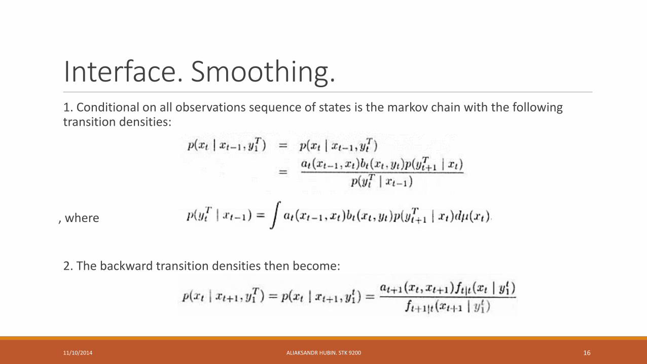
Interface. Smoothing.1. Conditional on all observations sequence of states is the markov chain with the following transition densities:

, where

2. The backward transition densities then become:


Interface. Smoothing.The smoothing densities are then computed with respect to the recursions in t:

and

,

where

5. Note that the joint density of the subsequence of states, which might be required at ML stage:


Recursion order


Inference on a function of states.6. It can also shown that having the smoothing distribution of the sequence of states it is easy to obtain the conditional expectation of some function assigned to the sequence, which can be recursively updated when a new observation becomes available (t>s):


Posterior mode estimationWe want to get the posterior mean of the states, namely:

Maximization of the posterior joint distribution of its states is invariant to being logorithmed:


Viterbi algorithmBecause of the special structure of the expression above the most likely value of 𝑥0 depends on only on 𝑥1 and after maximizing over 𝑥0, the most likely value of 𝑥1 depends only on 𝑥2 and so on, which leads to the following dynamic programming algorithm:

After which other values of the sequence are recovered in the following way:


Reference Probability MethodLet 𝑃 define the distribution when states and observations are independent with distribution g for the observations, then the following ratio can be derived:

And for any absolutely continuous measurable transformation 𝜙: 𝑥 → ℝ, we have (easy to compute):

On the other hand:


Reference Probability MethodWith

From the last expression on previous slide one can easily derive filtering recursions for the states of the model:

Thus, gives us an easy way to compute the filtering recursions for the states,

Even for the case when the time becomes continuous (e.g. differential equation model for states)


Forgetting initial distributionsLet us define the transition operator 𝐴∗and Bayes operator B:

and

Then the recursion densities which forget the initial distributions

if 𝐴∗ and B are contracting for some norm of densities.

It can be shown that initial distribution of the states is forgotten exponentially fast, and thus changes in filtering distributions and changes at fixed times disappear when the updates are made with the same observations.


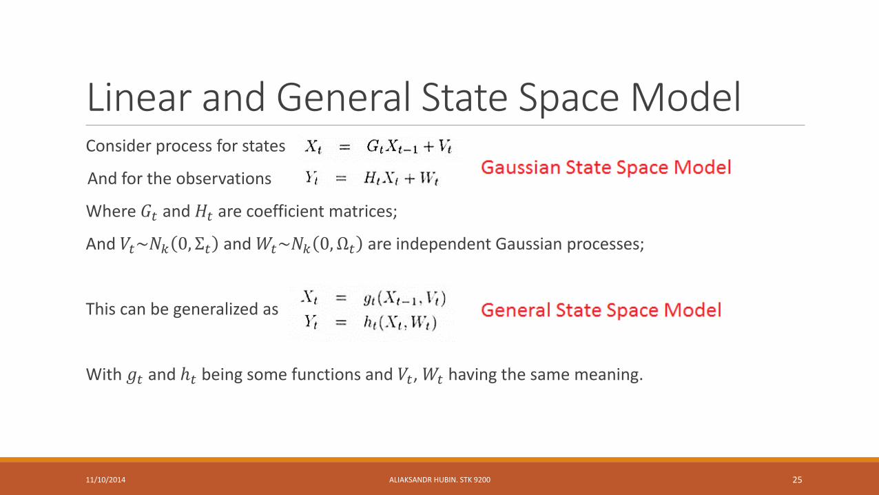
Linear and General State Space ModelConsider process for states

And for the observations

Where 𝐺𝑡 and 𝐻𝑡 are coefficient matrices;

And 𝑉𝑡~𝑁𝑘 0, Σ𝑡 and 𝑊𝑡~𝑁𝑘 0, Ω𝑡 are independent Gaussian processes;

This can be generalized as

With 𝑔𝑡 and ℎ𝑡 being some functions and 𝑉𝑡, 𝑊𝑡 having the same meaning.


Kalman filtering and SmoothingThen filtering densities for its hidden process look as follows:

Known as the so called Kalman Filter.

Kalman smoother correspondingly looks as follows:


Extended Kalman Filtering and SmoothingUse the standard Kalman filers and smoothers for the approximation of the process below:


General Cases• Use robust approximations for filtering and smoothing

• Use MCMC algorithms for filtering and smoothing


Parameter estimationLet state transitions 𝑎𝑡 depend on the vector of parameters 𝜏 and observation densities - 𝜂;

Let 𝜃 = {𝜏, 𝜂};

Then the following methods are usually addressed for estimation of 𝜃 in HMM:

Maximal likelihood method:

•EM(expectation-maximization)-algorithm, fast convergence to the neighborhood of the optimal value, extremely slow performance within this region;

• Newton's algorithm, slow convergence to the neighborhood of the optimal solution, good performance within it; Methaheuristics and/or Combinations of them can be applied.

Bayesian algorithms (Gibbs, Metropolis, etc.) can be applied after having set the priors for 𝜏and 𝜂. Full conditionals of posteriors are then as follows:


and

Parameter estimation ML


- Posterior joint probability of interest

- Likelihood function to be maximized

-Pdf of signal given statessequence

- Probability of the states' sequence

Where ℳ - is a model, s – is a sequence of states and X – is a set of the corresponding Observations.

Parameter estimation ML

Thus we are to maximize the likelihood of the model to estimate the parameters of interest:

Note that in general case the difficulty of these calculations is exponential 𝑂(𝑁𝑇), however in the efficient implementation the structure of the sequence of states yields into getting the polynomial difficulty algorithm.


Spatial-Temporal Model•Consider positions spatial-temporal positions t and their neighborhoods L(t) on 1…𝑇1 ×1…𝑇2 , with the following markov property 𝑃 𝑥 𝑡 𝑥 𝑢 , 𝑢 ≠ 𝑡 = 𝑃 𝑥 𝑡 𝑥 𝑢 , 𝑢 ∈ 𝐿(𝑡 )

•Then given the prior for x: 𝑃 𝑥𝐶 =1

𝑍 𝑐∈𝐶 𝑒

−Ф𝑐(𝑥𝑐) for any class C of non-empty complete

subsets of L

•The posterior for the state looks as:

•The joint distribution of the observation within given neighborhood:

•The joint density for the neighborhood:


Spatial-Temporal Model. Issues


Spatial-Temporal Model. Issues


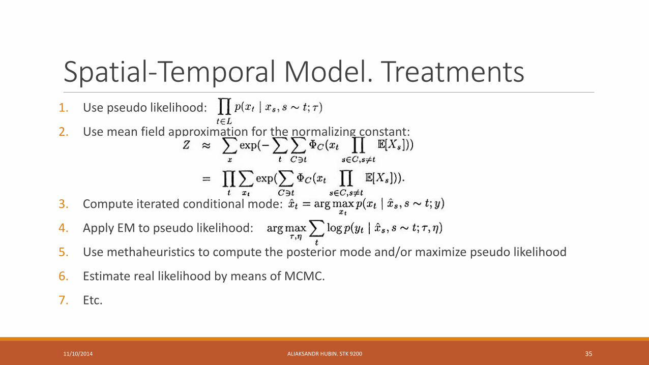
Spatial-Temporal Model. Treatments1. Use pseudo likelihood:

2. Use mean field approximation for the normalizing constant:

3. Compute iterated conditional mode:

4. Apply EM to pseudo likelihood:

5. Use methaheuristics to compute the posterior mode and/or maximize pseudo likelihood

6. Estimate real likelihood by means of MCMC.

7. Etc.


References

1. Kunsch, H.R., State Space and Hidden Markov Models. ETH-Zurich, Zurich;

2. Vaseghi, S. V., Hidden Markov Models. Wiley & Sons Ltd.


The End


Date post:	03-Jul-2020
Category:	Documents
Upload:	others
View:	1 times
Download:	0 times

Hidden Markov Models - Universitetet i oslo · Hidden Markov Models •The observations are...

Documents

Markov Models and Hidden Markov Models (HMMs)

L13: hidden Markov models - Texas A&M Universityresearch.cs.tamu.edu/prism/lectures/sp/l13.pdf · L13: hidden Markov models • Discrete Markov processes • Hidden Markov models

Introduction to Probabilistic Graphical Modelspub.ist.ac.at/~chl/courses/PGM_W16/part6.pdf · Inference in Hidden Markov Models Learning Hidden Markov Models Hidden Markov Models

Hidden Markov Models - uml.edugrinstei/91.510/HMM/Class Sildes - Hidden Markov... · Hidden Markov Models. ... particular hidden state. • Thus a hidden Markov model is a standard

Hidden Markov Models - AUusers-cs.au.dk/cstorm/courses/PRiB_f12/slides/hidden-markov-model… · Hidden Markov Models Markov Model Hidden Markov Model If the latent variables are

Markov Chains and Hidden Markov Models - Rice University · are “hidden”; hence, we have a hidden Markov model, or HMM. ... In Markov chains and hidden Markov models, the probability

L13: hidden Markov modelscourses.cs.tamu.edu/rgutier/csce630_f14/l13.pdf · L13: hidden Markov models • Discrete Markov processes • Hidden Markov models • Forward and Backward

EE365: Hidden Markov Models - Stanford Universityee266.stanford.edu/lectures/hmm.pdf · EE365: Hidden Markov Models Hidden Markov Models The Viterbi Algorithm 1. Hidden Markov Models

Hidden Markov Models - Home | Princeton Universityrvan/orf557/hmm080728.pdf · 1 Hidden Markov Models..... 1 1.1 Markov Processes ..... 1 1.2 Hidden Markov Models..... 4 ... able

Hidden Markov Models -

Bioinformatics Introduction to Hidden Markov Models - … · Bioinformatics Introduction to Hidden Markov Models Hidden Markov Models and Multiple Sequence Alignment Slides borrowed

Hidden Markov Models in Bioinformaticscsatol/mach_learn/bemutato/Mate_Korosi_HMMpr… · Outline ˜ Markov Chain ˜ HMM (Hidden Markov Model) ˜ Hidden Markov Models in Bioinformatics

Inference in Mixed Hidden Markov Models and Applications ... · 2. From hidden Markov models to mixed hidden Markov models Many authors suggested applying hidden Markov models to

9 Markov chains and Hidden Markov Models - Freie … · 9 Markov chains and Hidden Markov Models We will discuss: Markov chains Hidden Markov Models (HMMs) Algorithms: Viterbi, forward,

Hidden Markov Models and Gaussian Mixture Models · Hidden Markov Models and Gaussian Mixture Models ... Hidden Markov Model ... ASR Lectures 4&5 Hidden Markov Models and Gaussian

Hidden Markov Models./awm/tutorials/hmm14.pdf · Hidden Markov Models ... 14)

Overview Hidden Markov Models Gaussian Mixture Models · Hidden Markov Models and Gaussian Mixture Models ... Hidden Markov models HMM algorithms ... model ASR Lectures 4&5 Hidden