5 HIDDEN MARKOV MODELS 5.1 Statistical Models for Non-Stationary Processes 5.2 Hidden Markov Models 5.3 Training Hidden Markov Models 5.4 Decoding of Signals Using Hidden Markov Models 5.5 HMM-Based Estimation of Signals in Noise 5.6 Signal and Noise Model Combination and Decomposition 5.7 HMM-Based Wiener Filters 5.8 Summary
idden Markov models (HMMs) are used for the statistical modelling of non-stationary signal processes such as speech signals, image sequences and time-varying noise. An HMM models the time
variations (and/or the space variations) of the statistics of a random process with a Markovian chain of state-dependent stationary subprocesses. An HMM is essentially a Bayesian finite state process, with a Markovian prior for modelling the transitions between the states, and a set of state probability density functions for modelling the random variations of the signal process within each state. This chapter begins with a brief introduction to continuous and finite state non-stationary models, before concentrating on the theory and applications of hidden Markov models. We study the various HMM structures, the Baum–Welch method for the maximum-likelihood training of the parameters of an HMM, and the use of HMMs and the Viterbi decoding algorithm for the classification and decoding of an unlabelled observation signal sequence. Finally, applications of the HMMs for the enhancement of noisy signals are considered.
H
H E LL O
Advanced Digital Signal Processing and Noise Reduction, Second Edition.Saeed V. Vaseghi
5.1 Statistical Models for Non-Stationary Processes A non-stationary process can be defined as one whose statistical parameters vary over time. Most “naturally generated” signals, such as audio signals, image signals, biomedical signals and seismic signals, are non-stationary, in that the parameters of the systems that generate the signals, and the environments in which the signals propagate, change with time. A non-stationary process can be modelled as a double-layered stochastic process, with a hidden process that controls the time variations of the statistics of an observable process, as illustrated in Figure 5.1. In general, non-stationary processes can be classified into one of two broad categories:
(a) Continuously variable state processes. (b) Finite state processes.
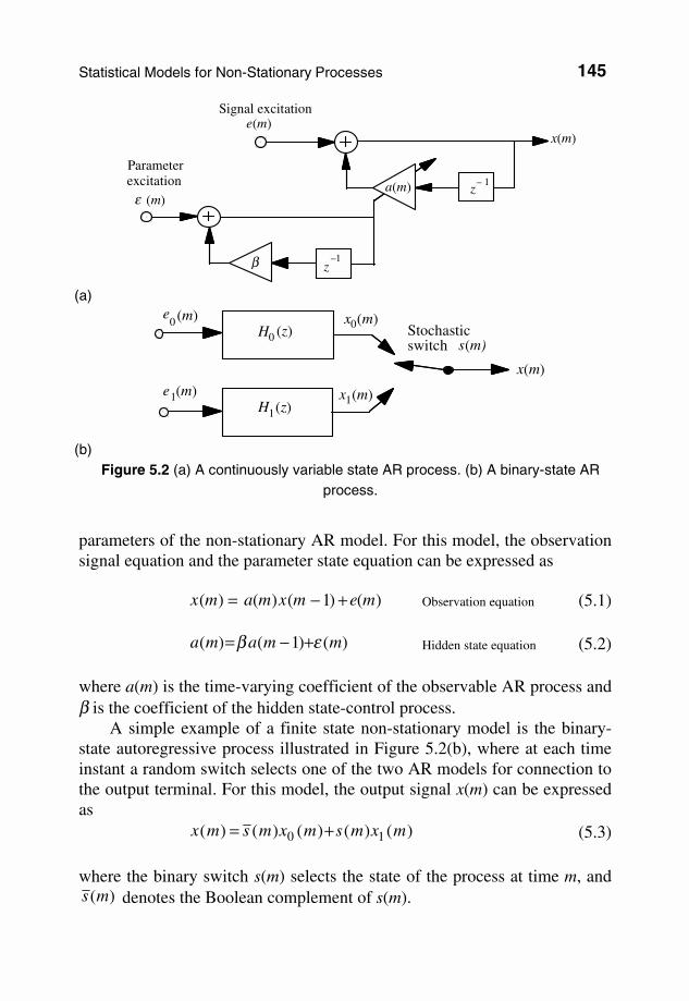
A continuously variable state process is defined as one whose underlying statistics vary continuously with time. Examples of this class of random processes are audio signals such as speech and music, whose power and spectral composition vary continuously with time. A finite state process is one whose statistical characteristics can switch between a finite number of stationary or non-stationary states. For example, impulsive noise is a binary-state process. Continuously variable processes can be approximated by an appropriate finite state process. Figure 5.2(a) illustrates a non-stationary first-order autoregressive (AR) process. This process is modelled as the combination of a hidden stationary AR model of the signal parameters, and an observable time-varying AR model of the signal. The hidden model controls the time variations of the
Hidden state-controlmodel
Observable process model
Processparameters
SignalExcitation
Figure 5.1 Illustration of a two-layered model of a non-stationary process.
Statistical Models for Non-Stationary Processes 145
parameters of the non-stationary AR model. For this model, the observation signal equation and the parameter state equation can be expressed as
where a(m) is the time-varying coefficient of the observable AR process and β is the coefficient of the hidden state-control process. A simple example of a finite state non-stationary model is the binary-state autoregressive process illustrated in Figure 5.2(b), where at each time instant a random switch selects one of the two AR models for connection to the output terminal. For this model, the output signal x(m) can be expressed as
)()()()()( 10 mxmsmxmsmx += (5.3) where the binary switch s(m) selects the state of the process at time m, and
)(ms denotes the Boolean complement of s(m).
z– 1
Signal excitation e(m)
Parameter excitation
ε (m)a(m)
x(m)
β z–1
(a)
H0 (z)e
0 (m)Stochastic switch s(m)
x(m)
H1(z)e 1(m)
x0(m)
x1(m)
(b)
Figure 5.2 (a) A continuously variable state AR process. (b) A binary-state AR process.
146 Hidden Markov Models
(a)
State1 State2
PW =0.8 PB =0.2 PW =0.6 PB =0.4
Hidden state selector
(b)
0.2
0.4
0.80.6
S1
S2
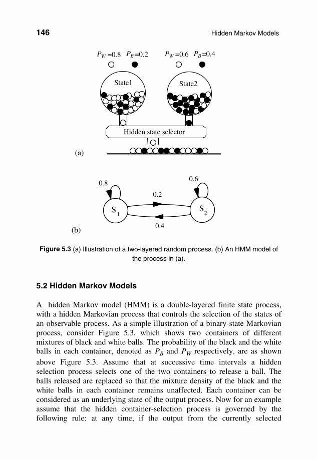
Figure 5.3 (a) Illustration of a two-layered random process. (b) An HMM model of
the process in (a).
5.2 Hidden Markov Models A hidden Markov model (HMM) is a double-layered finite state process, with a hidden Markovian process that controls the selection of the states of an observable process. As a simple illustration of a binary-state Markovian process, consider Figure 5.3, which shows two containers of different mixtures of black and white balls. The probability of the black and the white balls in each container, denoted as PB and PW respectively, are as shown above Figure 5.3. Assume that at successive time intervals a hidden selection process selects one of the two containers to release a ball. The balls released are replaced so that the mixture density of the black and the white balls in each container remains unaffected. Each container can be considered as an underlying state of the output process. Now for an example assume that the hidden container-selection process is governed by the following rule: at any time, if the output from the currently selected
Statistical Models for Non-Stationary Processes 147
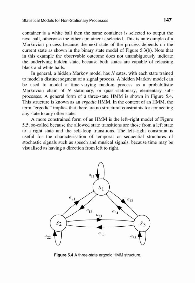
container is a white ball then the same container is selected to output the next ball, otherwise the other container is selected. This is an example of a Markovian process because the next state of the process depends on the current state as shown in the binary state model of Figure 5.3(b). Note that in this example the observable outcome does not unambiguously indicate the underlying hidden state, because both states are capable of releasing black and white balls. In general, a hidden Markov model has N sates, with each state trained to model a distinct segment of a signal process. A hidden Markov model can be used to model a time-varying random process as a probabilistic Markovian chain of N stationary, or quasi-stationary, elementary sub-processes. A general form of a three-state HMM is shown in Figure 5.4. This structure is known as an ergodic HMM. In the context of an HMM, the term “ergodic” implies that there are no structural constraints for connecting any state to any other state. A more constrained form of an HMM is the left–right model of Figure 5.5, so-called because the allowed state transitions are those from a left state to a right state and the self-loop transitions. The left–right constraint is useful for the characterisation of temporal or sequential structures of stochastic signals such as speech and musical signals, because time may be visualised as having a direction from left to right.
a12
a21
a23
a32
a31
a13
a11
a22 a33
S2 S3
S1
Figure 5.4 A three-state ergodic HMM structure.
148 Hidden Markov Models
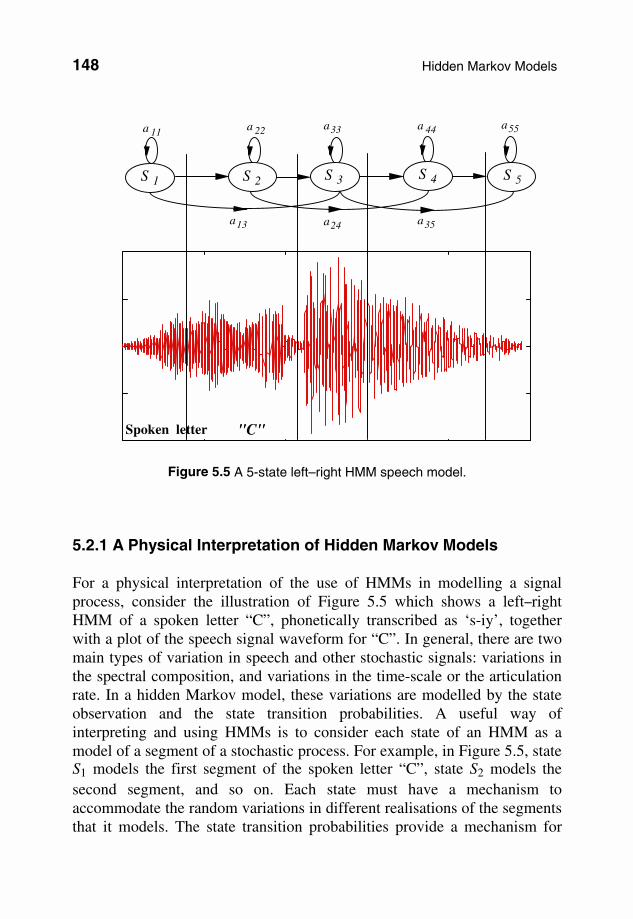
Figure 5.5 A 5-state left–right HMM speech model.
5.2.1 A Physical Interpretation of Hidden Markov Models For a physical interpretation of the use of HMMs in modelling a signal process, consider the illustration of Figure 5.5 which shows a left–right HMM of a spoken letter “C”, phonetically transcribed as ‘s-iy’, together with a plot of the speech signal waveform for “C”. In general, there are two main types of variation in speech and other stochastic signals: variations in the spectral composition, and variations in the time-scale or the articulation rate. In a hidden Markov model, these variations are modelled by the state observation and the state transition probabilities. A useful way of interpreting and using HMMs is to consider each state of an HMM as a model of a segment of a stochastic process. For example, in Figure 5.5, state S1 models the first segment of the spoken letter “C”, state S2 models the second segment, and so on. Each state must have a mechanism to accommodate the random variations in different realisations of the segments that it models. The state transition probabilities provide a mechanism for
S 1
a 11 a 22 a33 a 44 a55
a13 a24 a35
Spoken letter "C"
S 2 S 3 S 4 S 5
Hidden Markov Models 149
connection of various states, and for the modelling the variations in the duration and time-scales of the signals in each state. For example if a segment of a speech utterance is elongated, owing, say, to slow articulation, then this can be accommodated by more self-loop transitions into the state that models the segment. Conversely, if a segment of a word is omitted, owing, say, to fast speaking, then the skip-next-state connection accommodates that situation. The state observation pdfs model the probability distributions of the spectral composition of the signal segments associated with each state. 5.2.2 Hidden Markov Model as a Bayesian Model A hidden Markov model M is a Bayesian structure with a Markovian state transition probability and a state observation likelihood that can be either a discrete pmf or a continuous pdf. The posterior pmf of a state sequence s of a model M, given an observation sequence X, can be expressed using Bayes’ rule as the product of a state prior pmf and an observation likelihood function:
( )( )
( ) ( )MMM MMM s,XsX
X,s S,XSX
X,S |||1
fPf
P = (5.4)
where the observation sequence X is modelled by a probability density function PS|X,M(s|X,M).
The posterior probability that an observation signal sequence X was generated by the model M is summed over all likely state sequences, and may also be weighted by the model prior )(MMP :
( )( )
( ) ( )∑=s
S,X|SX
X s,XsX
X�� ��� ����������
likelihoodnObservatioriorpStateriorpModel
fPPf
P MMMM MMMM || )(1
(5.5)
The Markovian state transition prior can be used to model the time variations and the sequential dependence of most non-stationary processes. However, for many applications, such as speech recognition, the state observation likelihood has far more influence on the posterior probability than the state transition prior.
150 Hidden Markov Models
5.2.3 Parameters of a Hidden Markov Model A hidden Markov model has the following parameters: Number of states N. This is usually set to the total number of distinct, or
elementary, stochastic events in a signal process. For example, in modelling a binary-state process such as impulsive noise, N is set to 2, and in isolated-word speech modelling N is set between 5 to 10.
State transition-probability matrix A={aij, i,j=1, ... N}. This provides a
Markovian connection network between the states, and models the variations in the duration of the signals associated with each state. For a left–right HMM (see Figure 5.5), aij=0 for i>j, and hence the transition matrix A is upper-triangular.
State observation vectors {µi1, µi2, ..., µiM, i=1, ..., N}. For each state a set
of M prototype vectors model the centroids of the signal space associated with each state.
State observation vector probability model. This can be either a discrete model composed of the M prototype vectors and their associated probability mass function (pmf) P={Pij(· ); i=1, ..., N, j=1, ... M}, or it may be a continuous (usually Gaussian) pdf model F={fij(· ); i=1, ..., N, j=1, ..., M}.
Initial state probability vector π=[π1, π2, ..., πN]. 5.2.4 State Observation Models Depending on whether a signal process is discrete-valued or continuous-valued, the state observation model for the process can be either a discrete-valued probability mass function (pmf), or a continuous-valued probability density function (pdf). The discrete models can also be used for the modelling of the space of a continuous-valued process quantised into a number of discrete points. First, consider a discrete state observation density model. Assume that associated with the ith state of an HMM there are M discrete centroid vectors [µi1, ..., µiM] with a pmf [Pi1, ..., PiM]. These centroid vectors and their probabilities are normally obtained through clustering of a set of training signals associated with each state.
Hidden Markov Models 151
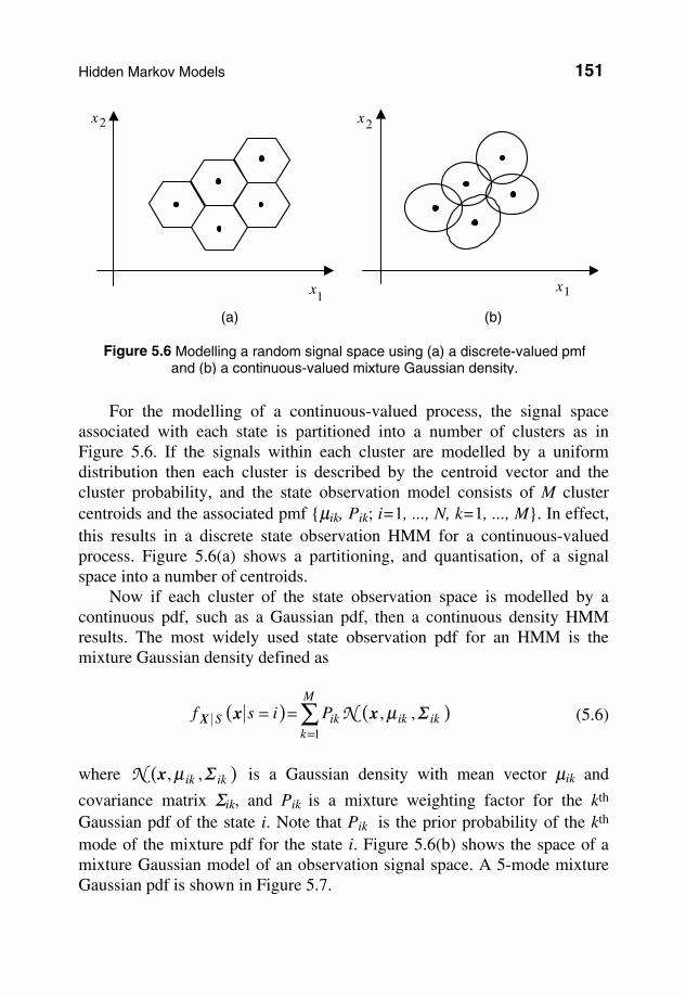
For the modelling of a continuous-valued process, the signal space associated with each state is partitioned into a number of clusters as in Figure 5.6. If the signals within each cluster are modelled by a uniform distribution then each cluster is described by the centroid vector and the cluster probability, and the state observation model consists of M cluster centroids and the associated pmf {µik, Pik; i=1, ..., N, k=1, ..., M}. In effect, this results in a discrete state observation HMM for a continuous-valued process. Figure 5.6(a) shows a partitioning, and quantisation, of a signal space into a number of centroids. Now if each cluster of the state observation space is modelled by a continuous pdf, such as a Gaussian pdf, then a continuous density HMM results. The most widely used state observation pdf for an HMM is the mixture Gaussian density defined as
( ) ( )∑=
==M
kikikikS Pisf
1
,, ΣµxxX N (5.6)
where ( )ikik Σµ ,,xN is a Gaussian density with mean vector µik and
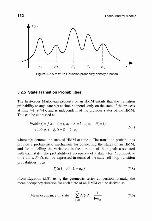
covariance matrix Σik, and Pik is a mixture weighting factor for the kth Gaussian pdf of the state i. Note that Pik is the prior probability of the kth mode of the mixture pdf for the state i. Figure 5.6(b) shows the space of a mixture Gaussian model of an observation signal space. A 5-mode mixture Gaussian pdf is shown in Figure 5.7.
x1
x2
x1
x2
(a) (b)
Figure 5.6 Modelling a random signal space using (a) a discrete-valued pmf and (b) a continuous-valued mixture Gaussian density.
152 Hidden Markov Models
5.2.5 State Transition Probabilities The first-order Markovian property of an HMM entails that the transition probability to any state s(t) at time t depends only on the state of the process at time t–1, s(t–1), and is independent of the previous states of the HMM. This can be expressed as
( )( ) ijaitsjtsProb
lNtsktsitsjtsProb
==−===−=−=−=
)1()(
)(,,)2(,)1()( �
(5.7)
where s(t) denotes the state of HMM at time t. The transition probabilities provide a probabilistic mechanism for connecting the states of an HMM, and for modelling the variations in the duration of the signals associated with each state. The probability of occupancy of a state i for d consecutive time units, Pi(d), can be expressed in terms of the state self-loop transition probabilities aii as
( ) ( )iidiii aadP −= − 11 (5.8)
From Equation (5.8), using the geometric series conversion formula, the mean occupancy duration for each state of an HMM can be derived as
iidi a
dPdi−
== ∑∞
= 1
1)(stateofoccupancyMean
0 (5.9)
µ 1 µ µ µ µ
f (x)
x2 3 4 5
Figure 5.7 A mixture Gaussian probability density function.
Hidden Markov Models 153
s1 s2 s3
s4
a13 a24
a11 a22 a33 a44
a12 a23 a34
(a)
s1
Time
Stat
es s2
s3
s4
(b)
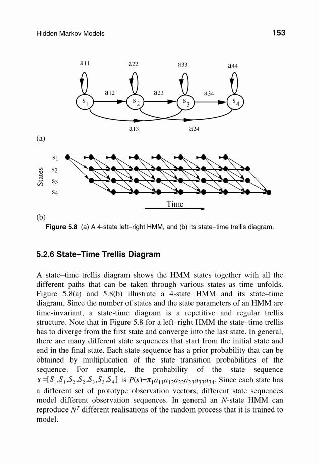
Figure 5.8 (a) A 4-state left–right HMM, and (b) its state–time trellis diagram.
5.2.6 State–Time Trellis Diagram A state–time trellis diagram shows the HMM states together with all the different paths that can be taken through various states as time unfolds. Figure 5.8(a) and 5.8(b) illustrate a 4-state HMM and its state–time diagram. Since the number of states and the state parameters of an HMM are time-invariant, a state-time diagram is a repetitive and regular trellis structure. Note that in Figure 5.8 for a left–right HMM the state–time trellis has to diverge from the first state and converge into the last state. In general, there are many different state sequences that start from the initial state and end in the final state. Each state sequence has a prior probability that can be obtained by multiplication of the state transition probabilities of the sequence. For example, the probability of the state sequence
],,,,,,[ 4332211 SSSSSSS=s is P(s)=π1a11a12a22a23a33a34. Since each state has a different set of prototype observation vectors, different state sequences model different observation sequences. In general an N-state HMM can reproduce NT different realisations of the random process that it is trained to model.
154 Hidden Markov Models
5.3 Training Hidden Markov Models The first step in training the parameters of an HMM is to collect a training database of a sufficiently large number of different examples of the random process to be modelled. Assume that the examples in a training database consist of L vector-valued sequences [X]=[Xk; k=0, ..., L–1], with each sequence Xk=[x(t); t=0, ..., Tk–1] having a variable number of Tk vectors. The objective is to train the parameters of an HMM to model the statistics of the signals in the training data set. In a probabilistic sense, the fitness of a model is measured by the posterior probability PM|X(M|X) of the model M
given the training data X. The training process aims to maximise the posterior probability of the model M and the training data [X], expressed using Bayes’ rule as
( )( )
( ) ( )MMM MMM Pff
PX
XX
X XX ||1= (5.10)
where the denominator fX(X) on the right-hand side of Equation (5.10) has only a normalising effect and PM(M) is the prior probability of the model M. For a given training data set [X] and a given model M, maximising Equation (5.10) is equivalent to maximising the likelihood function PX|M(X|M). The
likelihood of an observation vector sequence X given a model M can be expressed as
( ) ( ) ( )∑=s
sSXX ssXX MMM MMM |,|| , Pff (5.11)
where fX|S,M(X(t)|s(t),M), the pdf of the signal sequence X along the state
sequence 1)]((1)(0)[ −Ts,,s,s= �s of the model M, is given by
(5.12) where s(t), the state at time t, can be one of N states, and fX|S(X(t)|s(t)), a shorthand for fX|S,M(X(t)|s(t),M), is the pdf of x(t) given the state s(t) of the
model M. The Markovian probability of the state sequence s is given by
( ) 1)2)((2)(1)(1)(0)(0)| −− s(TTssssss aaa=P �πMM sS (5.13)
Training Hidden Markov Models 155
Substituting Equations (5.12) and (5.13) in Equation (5.11) yields
( )
( ) ( ) ( )∑
∑−−=
=
−−s
s
1)(1)((1)(1)(0)(0)
|(,||(
|1)(2)(|(1)(0)|(0)
|,||
TsTfasfa sf
)Pf)f
TsTssss xxx
ssXX
SXSXSX
sSXX
�π
MMM MMM
(5.14)
where the summation is taken over all state sequences s. In the training process, the transition probabilities and the parameters of the observation pdfs are estimated to maximise the model likelihood of Equation (5.14). Direct maximisation of Equation (5.14) with respect to the model parameters is a non-trivial task. Furthermore, for an observation sequence of length T vectors, the computational load of Equation (5.14) is O(NT). This is an impractically large load, even for such modest values as N=6 and T=30. However, the repetitive structure of the trellis state–time diagram of an HMM implies that there is a large amount of repeated computation in Equation (5.14) that can be avoided in an efficient implementation. In the next section we consider the forward-backward method of model likelihood calculation, and then proceed to describe an iterative maximum-likelihood model optimisation method. 5.3.1 Forward–Backward Probability Computation An efficient recursive algorithm for the computation of the likelihood function fX|M(X|M) is the forward–backward algorithm. The forward–
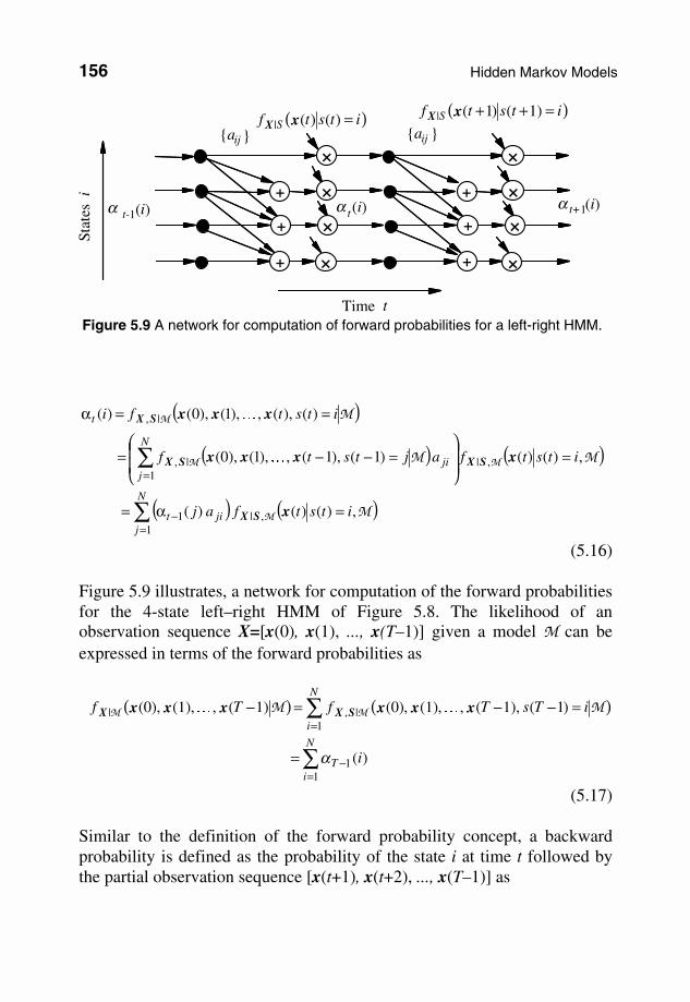
backward computation method exploits the highly regular and repetitive structure of the state–time trellis diagram of Figure 5.8. In this method, a forward probability variable αt(i) is defined as the joint probability of the partial observation sequence X=[x(0), x(1), ..., x(t)] and the state i at time t, of the model M:
The forward probability variable αt(i) of Equation (5.15) can be expressed in a recursive form in terms of the forward probabilities at time t–1, αt–1(i):
156 Hidden Markov Models
( )
( ) ( )
( ) ( )∑
∑
=−
=
=α=
=
=−−=
==α
N
jjit
ji
N
j
t
itstfaj
itstfajtstf
itstfi
1,|1
,|1
|,
|,
,)()( )(
,)()( )1( ),1(, ),1(),0(
)( ),(, ),1(),0( )(
M
MM
M
M
MM
M
x
xxxx
xxx
SX
SXSX
SX
�
�
(5.16)
Figure 5.9 illustrates, a network for computation of the forward probabilities for the 4-state left–right HMM of Figure 5.8. The likelihood of an observation sequence X=[x(0), x(1), ..., x(T–1)] given a model M can be expressed in terms of the forward probabilities as
( ) ( )
∑
∑
=−
=
=
=−−=−
N
iT
N
i
i
iTsTfTf
11
1|,|
)(
)1( ,1)(, ,(1),(0)1)(, ,(1),(0)
α
MM MM xxxxxx SXX ��
(5.17)
Similar to the definition of the forward probability concept, a backward probability is defined as the probability of the state i at time t followed by the partial observation sequence [x(t+1), x(t+2), ..., x(T–1)] as
{aij }
Time t
Stat
esi
α t-1(i) α t(i)+
α t+1(i)
+
+
×{aij }
+
+
+
×
×
× ×
×
×
×
( )itstf S =)()(| xX( )itstf S =++ 1)()1(| xX
Figure 5.9 A network for computation of forward probabilities for a left-right HMM.
Training Hidden Markov Models 157
( )
( )
( )
( )∑
∑
=+
=
=++=
=+×
−=+=
−==
N
jtij
N
jij
t
jtstfja
jts+tf
T+t+tjtsfa
T+t+titsfi
1|1
|
1,
,
)1()1()(
)1(1)(
1)(, ,)3(,)2(,)1(
)1(, 2),(,1)(,)( )(
M
M
M
M
M
M
,x
x
xxx
xxx
S,X
SX
SX
SX
β
β
,
�
�
(5.18)
In the next section, forward and backward probabilities are used to develop a method for the training of HMM parameters. 5.3.2 Baum–Welch Model Re-Estimation The HMM training problem is the estimation of the model parameters M=(π, A, F) for a given data set. These parameters are the initial state probabilities π, the state transition probability matrix A and the continuous (or discrete) density state observation pdfs. The HMM parameters are estimated from a set of training examples {X=[x(0), ..., x(T–1)]}, with the objective of maximising fX|M(X|M), the likelihood of the model and the
training data. The Baum–Welch method of training HMMs is an iterative likelihood maximisation method based on the forward–backward probabilities defined in the preceding section. The Baum–Welch method is an instance of the EM algorithm described in Chapter 4. For an HMM M, the posterior probability of a transition at time t from state i to state j of the model M, given an observation sequence X, can be expressed as
( )( )
( )( )
∑=
−
+=++=
=+==
=+==
N
iT
tSijt
t
i
jjtstfai
f
jtsitsf
jtsitsPji
11
1,|
|
|
,|
)(
)(,)1()1()(
,)1(,)(
,)1(,)( ),(
α
βα
γ
M
M
M
M
M
M
M
M
x
X
X
X
X
X
XS,
XS
(5.19)
where ( )MM XXS, ,)1(,)(| jtsitsf =+= is the joint pdf of the states s(t) and
158 Hidden Markov Models
s(t+1) and the observation sequence X, and ( )itstf S =++ )1()1(| xX is the state observation pdf for the state i. Note that for a discrete observation density HMM the state observation pdf in Equation (5.19) is replaced with the discrete state observation pmf ( )itstP S =++ )1()1(| xX . The posterior probability of state i at time t given the model M and the observation X is
( )( )
( )
∑=
−
=
==
==
N
jT
tt
t
j
ii
f
itsf
itsPi
11
|
|
,|
)(
)()(
,)(
,)( )(
α
βα
γ
M
M
M
M
M
M
X
X
X
X
XS,
XS
(5.20)
Now the state transition probability aij can be interpreted as
From Equations (5.19)–(5.21), the state transition probability can be re-estimated as the ratio
∑
∑−
=
−
==2
0
2
0
)(
),(
T
tt
T
tt
ij
i
ji
a
γ
γ
(5.22)
Note that for an observation sequence [x(0), ..., x(T–1)] of length T, the last transition occurs at time T–2 as indicated in the upper limits of the summations in Equation (5.22). The initial-state probabilities are estimated as
)(0 ii γπ = (5.23)
Training Hidden Markov Models 159
5.3.3 Training HMMs with Discrete Density Observation Models In a discrete density HMM, the observation signal space for each state is modelled by a set of discrete symbols or vectors. Assume that a set of M vectors [µi1,µi2, ..., µiM] model the space of the signal associated with the ith state. These vectors may be obtained from a clustering process as the centroids of the clusters of the training signals associated with each state. The objective in training discrete density HMMs is to compute the state transition probabilities and the state observation probabilities. The forward–backward equations for discrete density HMMs are the same as those for continuous density HMMs, derived in the previous sections, with the difference that the probability density functions such as ( )itstf S =)()(| xX
are substituted with probability mass functions ( )itstP S =)()(| xX defined
as ( ) ( )itstQPitstP SS === )()]([)()( || xx XX (5.24)
where the function Q[x(t)] quantises the observation vector x(t) to the nearest discrete vector in the set [µi1,µi2, ..., µiM]. For discrete density HMMs, the probability of a state vector µik can be defined as the ratio of the number of occurrences of µik (or vectors quantised to µik ) in the state i, divided by the total number of occurrences of all other vectors in the state i:
∑
∑−
=
−
→∈=
=
1
0
1
)(
)(
)(
stateintimesofnumberexpected
observingandstateintimesofnumberexpected)(
T
tt
T
ttt
ikikik
i
i
i
iP
ik
γ
γµ
µµ
x
(5.25)
In Equation (5.25) the summation in the numerator is taken over those time instants t where the kth symbol µik is observed in the state i. For statistically reliable results, an HMM must be trained on a large data set X consisting of a sufficient number of independent realisations of the process to be modelled. Assume that the training data set consists of L realisations X=[X(0), X(1), ..., X(L–1)], where X(k)=[x(0), x(1), ..., x(Tk–1)]. The re-estimation formula can be averaged over the entire data set as
160 Hidden Markov Models
∑−
==
1
00 )(
1ˆ
L
l
li i
Lγπ (5.26)
∑ ∑
∑ ∑−
=
−
=
−
=
−
==1
0
2
0
1
0
2
0
)(
),(
ˆL
l
T
t
lt
L
l
T
t
lt
ijl
l
i
ji
a
γ
γ
(5.27)
and
∑ ∑
∑ ∑−
=
−
=
−
=
−
→∈=1
0
1
0
1
0
1
)(
)(
)(
)(ˆL
l
T
t
lt
L
l
T
tt
lt
ikil
l
ik
i
i
P
γ
γµµ x
(5.28)
The parameter estimates of Equations (5.26)–(5.28) can be used in further iterations of the estimation process until the model converges. 5.3.4 HMMs with Continuous Density Observation Models In continuous density HMMs, continuous probability density functions (pdfs) are used to model the space of the observation signals associated with each state. Baum et al. generalised the parameter re-estimation method to HMMs with concave continuous pdfs such a Gaussian pdf. A continuous P-variate Gaussian pdf for the state i of an HMM can be defined as
( )( )
[ ] [ ]{ }iiii
PS ttitstf µΣµΣ
−−== − )()(exp2
1)()( 1T
2/12/xxxX
π (5.29)
where µi and Σi are the mean vector and the covariance matrix associated with the state i. The re-estimation formula for the mean vector of the state Gaussian pdf can be derived as
Training Hidden Markov Models 161
∑
∑−
=
−
==1
0
1
0
)(
)()(
T
tt
T
tt
i
i
ti
γ
γ x
µ (5.30)
Similarly, the covariance matrix is estimated as
( )( )
∑
∑−
=
−
=−−
=1
0
1
0
T
)(
)()()(
T
tt
T
tiit
i
i
tti
γ
γ µµΣ
xx
(5.31)
The proof that the Baum–Welch re-estimation algorithm leads to maximisation of the likelihood function fX|M(X|M) can be found in Baum.
5.3.5 HMMs with Mixture Gaussian pdfs The modelling of the space of a signal process with a mixture of Gaussian pdfs is considered in Section 4.5. In HMMs with mixture Gaussian pdf state models, the signal space associated with the ith state is modelled with a mixtures of M Gaussian densities as
( ) ( )∑=
==M
kikikikS tPitstf
1| ,,)()()( ΣµxxX N (5.32)
where Pik is the prior probability of the kth component of the mixture. The posterior probability of state i at time t and state j at time t+1 of the model M, given an observation sequence X=[x(0), ..., x(T–1)], can be expressed as
( )
( )
∑
∑
=−
+=
α
β
+α
=
=+==γ
N
iT
t
M
kjkjkjkijt
t
i
j)t(Pai
jtsitsPji
11
11
,|
)(
)(,,1)(
,|)1(,)( ),(
Σµx
XXS
N
MM
(5.33)
162 Hidden Markov Models
and the posterior probability of state i at time t given the model M and the observation X is given by
( )
∑=
−
=
==
N
jT
tt
t
j
ii
i)t(sPi
11
,|
)(
)()(
, )(
α
βα
γ MM XXS
(5.34)
Now we define the joint posterior probability of the state i and the kth
Gaussian mixture component pdf model of the state i at time t as
( )
( )
∑
∑
=−
=−
α
βα
=
===ζ
N
jT
N
jtikikikjit
KSt
j
itPaj
ktmitsPki
11
11
,|,
)(
)(,,)()(
,)(,)( ),(
Σµx
XX
N
MM
(5.35)
where m(t) is the Gaussian mixture component at time t. Equations (5.33) to (5.35) are used to derive the re-estimation formula for the mixture coefficients, the mean vectors and the covariance matrices of the state mixture Gaussian pdfs as
∑
∑−
=
−
==
=
1
0
1
0
)(
),(
stateintimesofnumberexpected
mixtureobservingandstateintimesofnumberexpected
T
tt
T
tt
ik
i
ki
i
kiP
γ
ξ (5.36)
and
∑
∑−
=
−
==1
0
1
0
),(
)(),(
T
tt
T
tt
ik
ki
tki
ξ
ξ x
µ (5.37)
Decoding of Signals Using Hidden Markov Models 163
Similarly the covariance matrix is estimated as
[ ][ ]
∑
∑−
=
−
=−−
=1
0
1
0
T
),(
)()(),(
T
tt
T
tikikt
ik
ki
ttki
ξ
ξ µµΣ
xx
(5.38)
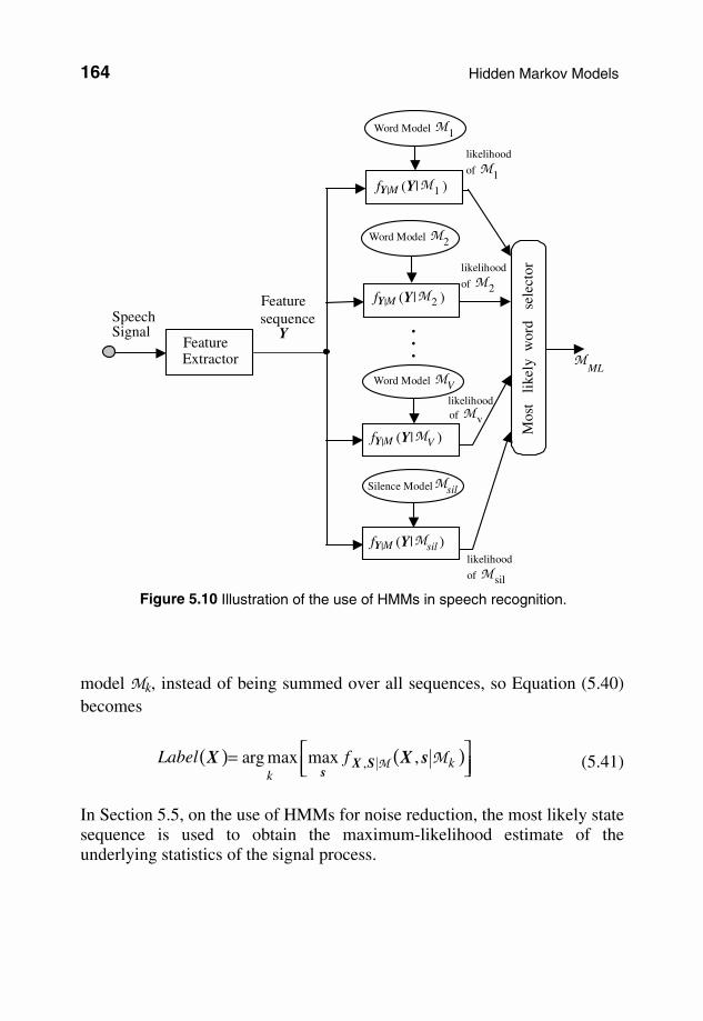
5.4 Decoding of Signals Using Hidden Markov Models Hidden Markov models are used in applications such as speech recognition, image recognition and signal restoration, and for the decoding of the underlying states of a signal. For example, in speech recognition, HMMs are trained to model the statistical variations of the acoustic realisations of the words in a vocabulary of say size V words. In the word recognition phase, an utterance is classified and labelled with the most likely of the V+1 candidate HMMs (including an HMM for silence) as illustrated in Figure 5.10. In Chapter 12 on the modelling and detection of impulsive noise, a binary–state HMM is used to model the impulsive noise process. Consider the decoding of an unlabelled sequence of T signal vectors X=[x(0), x(1), ..., X(T–1)] given a set of V candidate HMMs [M1 ,..., MV]. The probability score for the observation vector sequence X and the model Mk can be calculated as the likelihood:
where the likelihood of the observation sequence X is summed over all possible state sequences of the model M. Equation (5.39) can be efficiently calculated using the forward–backward method described in Section 5.3.1. The observation sequence X is labelled with the HMM that scores the highest likelihood as
In decoding applications often the likelihood of an observation sequence X and a model Mk is obtained along the single most likely state sequence of
164 Hidden Markov Models
model Mk, instead of being summed over all sequences, so Equation (5.40) becomes
( ) ( )
= k
kfLabel MM sXX SX
s,maxmaxarg , (5.41)
In Section 5.5, on the use of HMMs for noise reduction, the most likely state sequence is used to obtain the maximum-likelihood estimate of the underlying statistics of the signal process.
MML
.
.
.
Speech Signal
Feature sequence
Y
fY|M (Y|M1 )
Word Model M2
likelihood
of M2
Mos
t li
kely
wor
d s
elec
tor
Feature Extractor
Word Model MV
Word Model M1
fY|M (Y|M2 )
fY|M (Y|MV )
likelihood
of M1
likelihood of Mv
Silence Model Msil
fY|M (Y|Msil )likelihood
of M sil
Figure 5.10 Illustration of the use of HMMs in speech recognition.
Decoding of Signals Using Hidden Markov Models 165
5.4.1 Viterbi Decoding Algorithm In this section, we consider the decoding of a signal to obtain the maximum a posterior (MAP) estimate of the underlying state sequence. The MAP state sequence sMAP of a model M given an observation signal sequence X=[x(0), ..., x(T–1)] is obtained as
( )
( ) ( )( )MM
M
MM
M
ssX
sXs
SSXs
SXs
Pf
fMAP
,maxarg
,maxarg
,
,
=
=
(5.42)
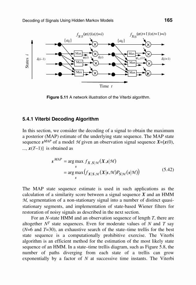
The MAP state sequence estimate is used in such applications as the calculation of a similarity score between a signal sequence X and an HMM M, segmentation of a non-stationary signal into a number of distinct quasi-stationary segments, and implementation of state-based Wiener filters for restoration of noisy signals as described in the next section. For an N-state HMM and an observation sequence of length T, there are altogether NT state sequences. Even for moderate values of N and T say (N=6 and T=30), an exhaustive search of the state–time trellis for the best state sequence is a computationally prohibitive exercise. The Viterbi algorithm is an efficient method for the estimation of the most likely state sequence of an HMM. In a state–time trellis diagram, such as Figure 5.8, the number of paths diverging from each state of a trellis can grow exponentially by a factor of N at successive time instants. The Viterbi
{aij}
Time t
Stat
esi
fX|S (x(t)|s(t)=i) fX|S
×Max
Max
Max
x
×
×
×
(x(t+1)|s(t+1)=i)
{aij}
×Max
Max
Max
×
×
×
ψt(i) ψt+1(i)δt(i) δt(i+1)δt(i–1)
Figure 5.11 A network illustration of the Viterbi algorithm.
166 Hidden Markov Models
method prunes the trellis by selecting the most likely path to each state. At each time instant t, for each state i, the algorithm selects the most probable path to state i and prunes out the less likely branches. This procedure ensures that at any time instant, only a single path survives into each state of the trellis.
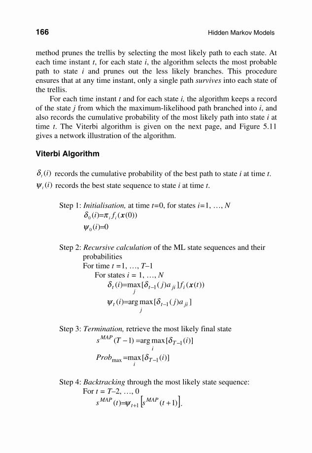
For each time instant t and for each state i, the algorithm keeps a record of the state j from which the maximum-likelihood path branched into i, and also records the cumulative probability of the most likely path into state i at time t. The Viterbi algorithm is given on the next page, and Figure 5.11 gives a network illustration of the algorithm. Viterbi Algorithm
)(itδ records the cumulative probability of the best path to state i at time t.
)(itψ records the best state sequence to state i at time t. Step 1: Initialisation, at time t=0, for states i=1, …, N ))0(()(0 xii fi πδ =
0)(0 =iψ Step 2: Recursive calculation of the ML state sequences and their probabilities For time t =1, …, T–1 For states i = 1, …, N ))((])([max)( 1 tfaji ijit
jt x−= δδ
])([maxarg)( 1 jitj
t aji −= δψ
Step 3: Termination, retrieve the most likely final state
)]([maxarg)1( 1 iTs Ti
MAP−=− δ
)]([max 1max iProb Ti
−= δ
Step 4: Backtracking through the most likely state sequence: For t = T–2, …, 0
[ ])1()( 1 += + tsts MAPt
MAP ψ .
HMM-Based Estimation of Signals in Noise 167
The backtracking routine retrieves the most likely state sequence of the model M. Note that the variable Probmax, which is the probability of the observation sequence X=[x(0), ..., x(T–1)] and the most likely state sequence of the model M, can be used as the probability score for the model
M and the observation X. For example, in speech recognition, for each candidate word model the probability of the observation and the most likely state sequence is calculated, and then the observation is labelled with the word that achieves the highest probability score. 5.5 HMM-Based Estimation of Signals in Noise In this section, and the following two sections, we consider the use of HMMs for estimation of a signal x(t) observed in an additive noise n(t), and modelled as
)()()( ttt nxy += (5.43) From Bayes’ rule, the posterior pdf of the signal x(t) given the noisy observation y(t) is defined as
( )( )
( ) ( ))()()())((
1
))((
))(()()()()( |
|
tfttftf
tf
tfttfttf
Y
xxyy
y
xxyyx
XNY
XXYYX
−=
= (5.44)
For a given observation, fY(y(t)) is a constant, and the maximum a posteriori (MAP) estimate is obtained as
( ) ( ))()()(maxarg)(ˆ)(
tfttftMAP xxyx XNtx
−= (5.45)
The computation of the posterior pdf, Equation (5.44), or the MAP estimate Equation (5.45), requires the pdf models of the signal and the noise processes. Stationary, continuous-valued, processes are often modelled by a Gaussian or a mixture Gaussian pdf that is equivalent to a single-state HMM. For a non-stationary process an N-state HMM can model the time-
168 Hidden Markov Models
varying pdf of the process as a Markovian chain of N stationary Gaussian subprocesses. Now assume that we have an Ns-state HMM M for the signal, and another Nn-state HMM η for the noise. For signal estimation, we need estimates of the underlying state sequences of the signal and the noise
processes. For an observation sequence of length T, there are TsN possible
signal state sequences and TnN possible noise state sequences that could
have generated the noisy signal. Since it is assumed that the signal and noise are uncorrelated, each signal state may be observed in any noisy state;
therefore the number of noisy signal states is on the order of TsN × T
nN . Given an observation sequence Y=[y(0), y(1), ..., y(T–1)], the most probable state sequences of the signal and the noise HMMs maybe expressed as
( )
= η,,,maxmaxarg noisesignalsignal
noisesignal
MssYs Yss
fMAP (5.46)
and
( )
= η,,,maxmaxarg noisesignalnoise
signalnoise
MssYs Yss
fMAP (5.47)
Given the state sequence estimates for the signal and the noise models, the MAP estimation Equation (5.45) becomes
( ) ( )( )MM ,)()()(maxarg)(ˆ signal,noiseMAP
XMAP
,MAP tf,ttft sxsxyx SSN
xηη −= (5.48)
Implementation of Equations (5.46)–(5.48) is computationally prohibitive. In Sections 5.6 and 5.7, we consider some practical methods for the estimation of signal in noise. Example Assume a signal, modelled by a binary-state HMM, is observed in an additive stationary Gaussian noise. Let the noisy observation be modelled as
)()()()()()( 10 tttsttst nxxy ++= (5.49) where s(t) is a hidden binary-state process such that: s(t) = 0 indicates that
HMM-Based Estimation of Signals in Noise 169
the signal is from the state S0 with a Gaussian pdf of )(000
,),( xxxx ΣµtN ,
and s(t) = 1 indicates that the signal is from the state S1 with a Gaussian pdf
of )(111
,),( xxxx ΣµtN . Assume that a stationary Gaussian process
)( ,),( nnnt ΣµnN , equivalent to a single-state HMM, can model the noise.
Using the Viterbi algorithm the maximum a posteriori (MAP) state sequence of the signal model can be estimated as
( ) ( )[ ]MM MM ssYs SSYs
PfMAP ,maxarg ,|signal = (5.50)
For a Gaussian-distributed signal and additive Gaussian noise, the observation pdf of the noisy signal is also Gaussian. Hence, the state observation pdfs of the signal model can be modified to account for the additive noise as
( ) ( ))(,)(),()(0000 0| nnxxnxY yy ΣΣµµ ++= tstf s N (5.51)
and ( ) ( ))(,)(),()(
1111 1| nnxxnxY yy ΣΣµµ ++= tstf s N (5.52)
where ( )Σµ,),(tyN
denotes a Gaussian pdf with mean vector µ and
covariance matrix Σ . The MAP signal estimate, given a state sequence estimate sMAP, is obtained from
( ) ( ) ( )[ ])()(,)(maxargˆ ,| ttftft MAPS
MAP xysxx NXx
−= MM (5.53)
Substitution of the Gaussian pdf of the signal from the most likely state sequence, and the pdf of noise, in Equation (5.53) results in the following MAP estimate:
ˆ x MAP(t ) = Σ xx ,s(t ) + Σnn( )−1Σ xx,s(t ) y( t) − µ n( ) + Σ xx ,s( t) + Σnn( )−1
Σ nn µ x,s(t )
(5.54)
where µ x,s(t) and Σ xx ,s( t) are the mean vector and covariance matrix of the
signal x(t) obtained from the most likely state sequence [s(t)].
170 Hidden Markov Models
Noisy speech
SpeechHMMs
Model
combination
NoiseHMMs
State
decomposition
Noisy speechHMMs
Speechstates
Noisestates
Wienerfilter
Speech
Noise
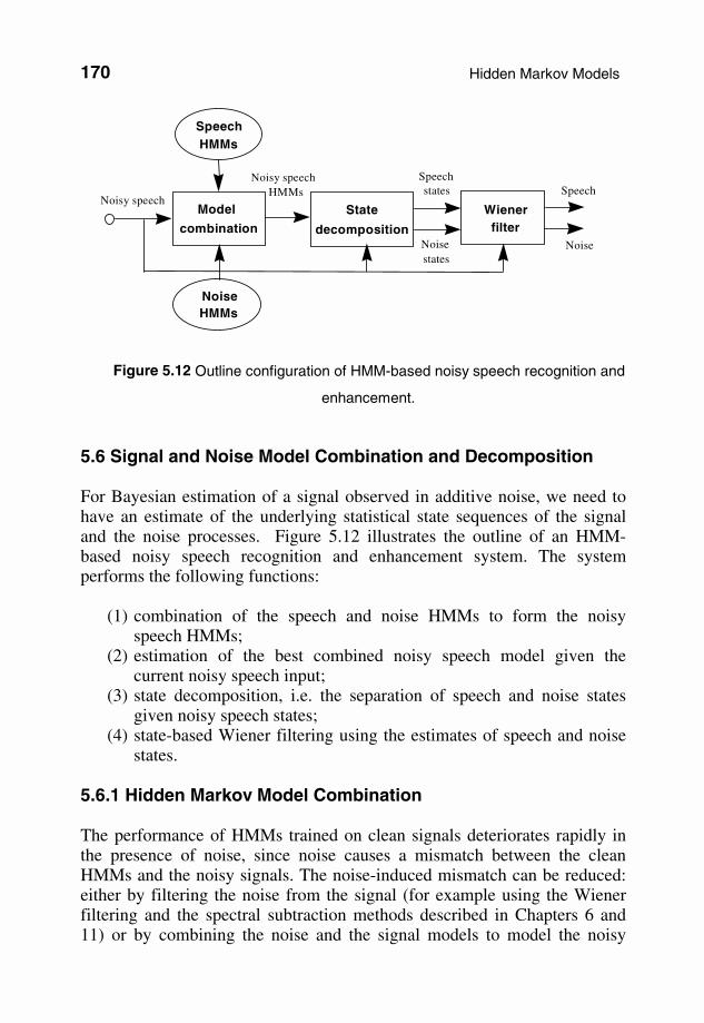
Figure 5.12 Outline configuration of HMM-based noisy speech recognition and
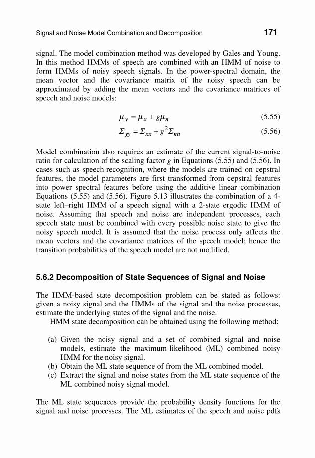
enhancement. 5.6 Signal and Noise Model Combination and Decomposition For Bayesian estimation of a signal observed in additive noise, we need to have an estimate of the underlying statistical state sequences of the signal and the noise processes. Figure 5.12 illustrates the outline of an HMM-based noisy speech recognition and enhancement system. The system performs the following functions:
(1) combination of the speech and noise HMMs to form the noisy speech HMMs;
(2) estimation of the best combined noisy speech model given the current noisy speech input;
(3) state decomposition, i.e. the separation of speech and noise states given noisy speech states;
(4) state-based Wiener filtering using the estimates of speech and noise states.
5.6.1 Hidden Markov Model Combination The performance of HMMs trained on clean signals deteriorates rapidly in the presence of noise, since noise causes a mismatch between the clean HMMs and the noisy signals. The noise-induced mismatch can be reduced: either by filtering the noise from the signal (for example using the Wiener filtering and the spectral subtraction methods described in Chapters 6 and 11) or by combining the noise and the signal models to model the noisy
Signal and Noise Model Combination and Decomposition 171
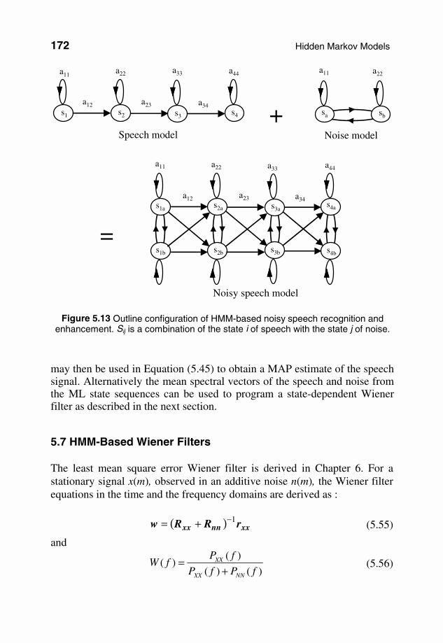
signal. The model combination method was developed by Gales and Young. In this method HMMs of speech are combined with an HMM of noise to form HMMs of noisy speech signals. In the power-spectral domain, the mean vector and the covariance matrix of the noisy speech can be approximated by adding the mean vectors and the covariance matrices of speech and noise models:
nxy µµµ g+= (5.55)
nnxxyy ΣΣΣ 2g+= (5.56)
Model combination also requires an estimate of the current signal-to-noise ratio for calculation of the scaling factor g in Equations (5.55) and (5.56). In cases such as speech recognition, where the models are trained on cepstral features, the model parameters are first transformed from cepstral features into power spectral features before using the additive linear combination Equations (5.55) and (5.56). Figure 5.13 illustrates the combination of a 4-state left–right HMM of a speech signal with a 2-state ergodic HMM of noise. Assuming that speech and noise are independent processes, each speech state must be combined with every possible noise state to give the noisy speech model. It is assumed that the noise process only affects the mean vectors and the covariance matrices of the speech model; hence the transition probabilities of the speech model are not modified. 5.6.2 Decomposition of State Sequences of Signal and Noise The HMM-based state decomposition problem can be stated as follows: given a noisy signal and the HMMs of the signal and the noise processes, estimate the underlying states of the signal and the noise. HMM state decomposition can be obtained using the following method:
(a) Given the noisy signal and a set of combined signal and noise models, estimate the maximum-likelihood (ML) combined noisy HMM for the noisy signal.
(b) Obtain the ML state sequence of from the ML combined model. (c) Extract the signal and noise states from the ML state sequence of the
ML combined noisy signal model.
The ML state sequences provide the probability density functions for the signal and noise processes. The ML estimates of the speech and noise pdfs
172 Hidden Markov Models
may then be used in Equation (5.45) to obtain a MAP estimate of the speech signal. Alternatively the mean spectral vectors of the speech and noise from the ML state sequences can be used to program a state-dependent Wiener filter as described in the next section. 5.7 HMM-Based Wiener Filters
The least mean square error Wiener filter is derived in Chapter 6. For a stationary signal x(m), observed in an additive noise n(m), the Wiener filter equations in the time and the frequency domains are derived as :
( ) xxnnxx rRRw 1−+= (5.55)
and
)()(
)()(
fPfP
fPfW
NN
XX
+=
XX
(5.56)
s1 s2 s3 s4
a11 a22 a33 a44
a12 a23 a34
s1b
a11 a22 a33 a44
a12 a34
s3b s4b
s4as3as2as1a
s2b
a23
+Speech model Noise model
Noisy speech model
=
sb
a22
sa
a11
Figure 5.13 Outline configuration of HMM-based noisy speech recognition and enhancement. Sij is a combination of the state i of speech with the state j of noise.
HMM-Based Wiener Filters 173
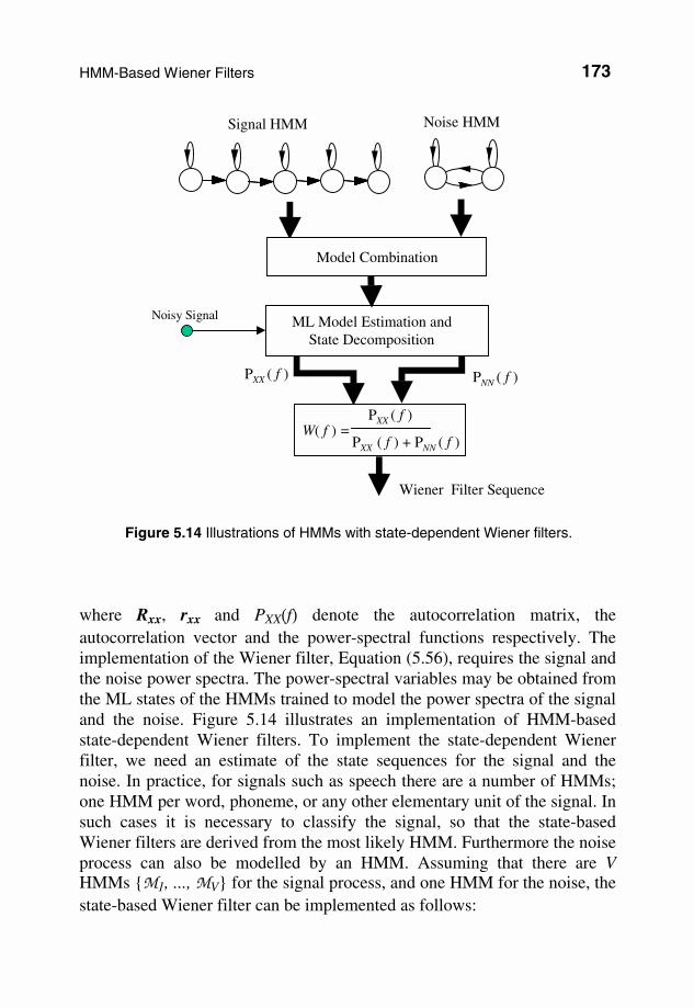
where Rxx, rxx and PXX(f) denote the autocorrelation matrix, the autocorrelation vector and the power-spectral functions respectively. The implementation of the Wiener filter, Equation (5.56), requires the signal and the noise power spectra. The power-spectral variables may be obtained from the ML states of the HMMs trained to model the power spectra of the signal and the noise. Figure 5.14 illustrates an implementation of HMM-based state-dependent Wiener filters. To implement the state-dependent Wiener filter, we need an estimate of the state sequences for the signal and the noise. In practice, for signals such as speech there are a number of HMMs; one HMM per word, phoneme, or any other elementary unit of the signal. In such cases it is necessary to classify the signal, so that the state-based Wiener filters are derived from the most likely HMM. Furthermore the noise process can also be modelled by an HMM. Assuming that there are V HMMs {M1, ..., MV} for the signal process, and one HMM for the noise, the state-based Wiener filter can be implemented as follows:
Signal HMM Noise HMM
Wiener Filter Sequence
PXX ( f )
Noisy Signal
PNN ( f )
ML Model Estimation and State Decomposition
W( f ) = PXX ( f )
PXX ( f ) + PNN ( f )
Model Combination
Figure 5.14 Illustrations of HMMs with state-dependent Wiener filters.
174 Hidden Markov Models
Step 1: Combine the signal and noise models to form the noisy signal
models. Step 2: Given the noisy signal, and the set of combined noisy signal
models, obtain the ML combined noisy signal model. Step 3: From the ML combined model, obtain the ML state sequence of
speech and noise. Step 4: Use the ML estimate of the power spectra of the signal and the
noise to program the Wiener filter Equation (5.56). Step 5: Use the state-dependent Wiener filters to filter the signal.
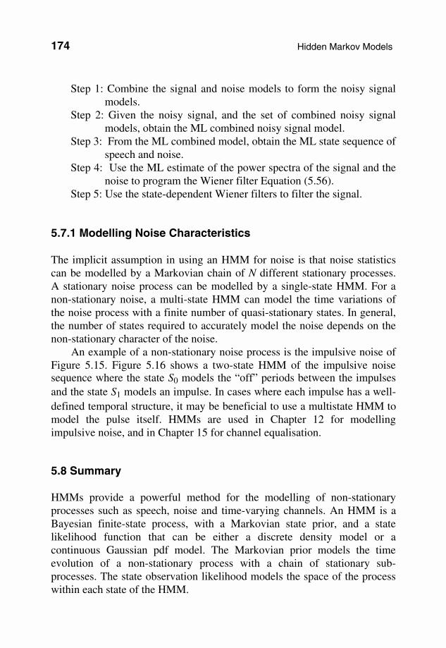
5.7.1 Modelling Noise Characteristics The implicit assumption in using an HMM for noise is that noise statistics can be modelled by a Markovian chain of N different stationary processes. A stationary noise process can be modelled by a single-state HMM. For a non-stationary noise, a multi-state HMM can model the time variations of the noise process with a finite number of quasi-stationary states. In general, the number of states required to accurately model the noise depends on the non-stationary character of the noise.
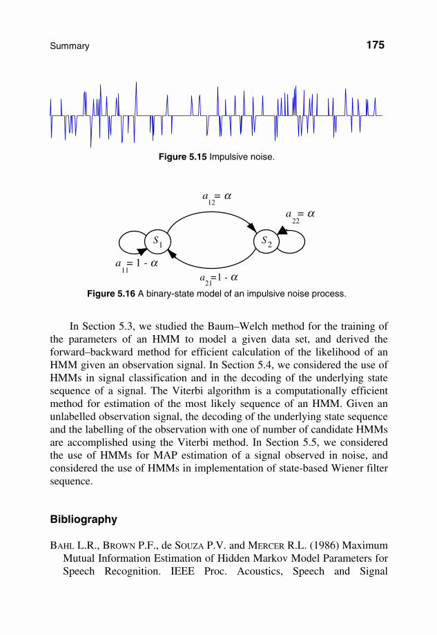
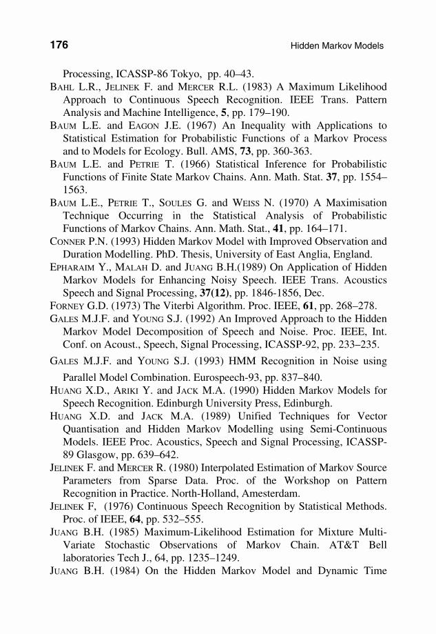
An example of a non-stationary noise process is the impulsive noise of Figure 5.15. Figure 5.16 shows a two-state HMM of the impulsive noise sequence where the state S0 models the “off” periods between the impulses and the state S1 models an impulse. In cases where each impulse has a well-defined temporal structure, it may be beneficial to use a multistate HMM to model the pulse itself. HMMs are used in Chapter 12 for modelling impulsive noise, and in Chapter 15 for channel equalisation. 5.8 Summary HMMs provide a powerful method for the modelling of non-stationary processes such as speech, noise and time-varying channels. An HMM is a Bayesian finite-state process, with a Markovian state prior, and a state likelihood function that can be either a discrete density model or a continuous Gaussian pdf model. The Markovian prior models the time evolution of a non-stationary process with a chain of stationary sub-processes. The state observation likelihood models the space of the process within each state of the HMM.
Summary 175
In Section 5.3, we studied the Baum–Welch method for the training of the parameters of an HMM to model a given data set, and derived the forward–backward method for efficient calculation of the likelihood of an HMM given an observation signal. In Section 5.4, we considered the use of HMMs in signal classification and in the decoding of the underlying state sequence of a signal. The Viterbi algorithm is a computationally efficient method for estimation of the most likely sequence of an HMM. Given an unlabelled observation signal, the decoding of the underlying state sequence and the labelling of the observation with one of number of candidate HMMs are accomplished using the Viterbi method. In Section 5.5, we considered the use of HMMs for MAP estimation of a signal observed in noise, and considered the use of HMMs in implementation of state-based Wiener filter sequence. Bibliography BAHL L.R., BROWN P.F., de SOUZA P.V. and MERCER R.L. (1986) Maximum
Mutual Information Estimation of Hidden Markov Model Parameters for Speech Recognition. IEEE Proc. Acoustics, Speech and Signal
Figure 5.15 Impulsive noise.
a = 1 - α11
12
21
a = α22
a = α
a =1 - α
S S21
Figure 5.16 A binary-state model of an impulsive noise process.
176 Hidden Markov Models
Processing, ICASSP-86 Tokyo, pp. 40–43. BAHL L.R., JELINEK F. and MERCER R.L. (1983) A Maximum Likelihood
Approach to Continuous Speech Recognition. IEEE Trans. Pattern Analysis and Machine Intelligence, 5, pp. 179–190.
BAUM L.E. and EAGON J.E. (1967) An Inequality with Applications to Statistical Estimation for Probabilistic Functions of a Markov Process and to Models for Ecology. Bull. AMS, 73, pp. 360-363.
BAUM L.E. and PETRIE T. (1966) Statistical Inference for Probabilistic Functions of Finite State Markov Chains. Ann. Math. Stat. 37, pp. 1554–1563.
BAUM L.E., PETRIE T., SOULES G. and WEISS N. (1970) A Maximisation Technique Occurring in the Statistical Analysis of Probabilistic Functions of Markov Chains. Ann. Math. Stat., 41, pp. 164–171.
CONNER P.N. (1993) Hidden Markov Model with Improved Observation and Duration Modelling. PhD. Thesis, University of East Anglia, England.
EPHARAIM Y., MALAH D. and JUANG B.H.(1989) On Application of Hidden Markov Models for Enhancing Noisy Speech. IEEE Trans. Acoustics Speech and Signal Processing, 37(12), pp. 1846-1856, Dec.
FORNEY G.D. (1973) The Viterbi Algorithm. Proc. IEEE, 61, pp. 268–278. GALES M.J.F. and YOUNG S.J. (1992) An Improved Approach to the Hidden
Markov Model Decomposition of Speech and Noise. Proc. IEEE, Int. Conf. on Acoust., Speech, Signal Processing, ICASSP-92, pp. 233–235.
GALES M.J.F. and YOUNG S.J. (1993) HMM Recognition in Noise using
Parallel Model Combination. Eurospeech-93, pp. 837–840. HUANG X.D., ARIKI Y. and JACK M.A. (1990) Hidden Markov Models for
Speech Recognition. Edinburgh University Press, Edinburgh. HUANG X.D. and JACK M.A. (1989) Unified Techniques for Vector
Quantisation and Hidden Markov Modelling using Semi-Continuous Models. IEEE Proc. Acoustics, Speech and Signal Processing, ICASSP-89 Glasgow, pp. 639–642.
JELINEK F. and MERCER R. (1980) Interpolated Estimation of Markov Source Parameters from Sparse Data. Proc. of the Workshop on Pattern Recognition in Practice. North-Holland, Amesterdam.
JELINEK F, (1976) Continuous Speech Recognition by Statistical Methods. Proc. of IEEE, 64, pp. 532–555.
JUANG B.H. (1985) Maximum-Likelihood Estimation for Mixture Multi-Variate Stochastic Observations of Markov Chain. AT&T Bell laboratories Tech J., 64, pp. 1235–1249.
JUANG B.H. (1984) On the Hidden Markov Model and Dynamic Time
Bibliography 177
Warping for Speech Recognition- A unified Overview. AT&T Technical J., 63, pp. 1213–1243.
KULLBACK S. and LEIBLER R.A. (1951) On Information and Sufficiency. Ann. Math. Stat., 22, pp. 79–85.
LEE K.F. (1989) Automatic Speech Recognition: the Development of SPHINX System. MA: Kluwer Academic Publishers, Boston.
LEE K.F. (1989) Hidden Markov Model: Past, Present and Future. Eurospeech-89, Paris.
LIPORACE L.R. (1982) Maximum Likelihood Estimation for Multi-Variate Observations of Markov Sources. IEEE Trans. IT, IT-28, pp. 729–735.
MARKOV A.A. (1913) An Example of Statistical Investigation in the text of Eugen Onyegin Illustrating Coupling of Tests in Chains. Proc. Acad. Sci. St Petersburg VI Ser., 7, pp. 153–162.
MILNER B.P. (1995) Speech Recognition in Adverse Environments, PhD. Thesis, University of East Anglia, England.
PETERIE T. (1969) Probabilistic Functions of Finite State Markov Chains. Ann. Math. Stat., 40, pp. 97–115.
RABINER L.R. and JUANG B.H. (1986) An Introduction to Hidden Markov Models. IEEE ASSP. Magazine, pp. 4–15.
RABINER L.R., JUANG B.H., LEVINSON S.E. and SONDHI M.M., (1985) Recognition of Isolated Digits using Hidden Markov Models with Continuous Mixture Densities. AT&T Technical Journal, 64, pp. 1211-1235.
RABINER L.R. and JUANG B.H. (1993) Fundamentals of Speech Recognition. Prentice-Hall, Englewood Cliffs, NJ.
YOUNG S.J. (1999), HTK: Hidden Markov Model Tool Kit. Cambridge University Engineering Department.
VARGA A. and MOORE R.K., Hidden Markov Model Decomposition of Speech and Noise. in Proc. IEEE Int., Conf. on Acoust., Speech, Signal Processing, 1990, pp. 845–848
VITERBI A.J. (1967) Error Bounds for Convolutional Codes and an Asymptotically Optimum Decoding Algorithm. IEEE Trans. on Information theory, IT-13, pp. 260–269.