Approximate Bayesian computation (ABC) is a powerful technique for estimating the posterior dis-tribution of a model’s parameters. It is especially important when the model to be fit has no explicitlikelihood function, which happens for computational (or simulation-based) models such as those thatare popular in cognitive neuroscience and other areas in psychology. However, ABC is usually appliedonly to models with few parameters. Extending ABC to hierarchical models has been difficult becausehigh-dimensional hierarchical models add computational complexity that conventional ABC cannot ac-commodate. In this paper, we summarize some current approaches for performing hierarchical ABC andintroduce a new algorithm called Gibbs ABC. This new algorithm incorporates well-known Bayesian tech-niques to improve the accuracy and efficiency of the ABC approach for estimation of hierarchical models.We then use the Gibbs ABC algorithm to estimate the parameters of two models of signal detection, onewith and one without a tractable likelihood function.
Key words: approximate Bayesian computation, hierarchical Bayesian estimation, signal detection the-ory, dynamic signal detection.
1. Introduction
Recently, there has been great interest in Bayesian estimation techniques, and our work(Turner & Van Zandt, 2012; Turner, Dennis, & Van Zandt, 2013; Turner & Sederberg, 2012) hasfocused on a particular approach called approximate Bayesian computation (ABC). The goal ofthis paper is to demonstrate how ABC can be applied to hierarchical models, in which the data-generating mechanisms for subjects are nested within a larger global structure that restricts theparameters for each subject.
To make the concepts that we will discuss more clear, we will orient our presentation aroundthe classic model of signal detection theory (SDT; e.g., Green & Swets, 1966; Egan, 1958). Wechose SDT as our working example because it is simple, well known in experimental psychol-ogy, and also because the classic SDT model can be contrasted with a more recent approachfor which explicit predictions are difficult to derive (Turner, Van Zandt, & Brown, 2011). Suchmodels, those without analytic expressions to describe their output, are usually explored by wayof simulation and are the kinds of models for which ABC was designed. Note, however, thatthe techniques we present in this paper are applicable to a wide variety of models, and are notintended to be restricted to SDT alone.
1.1. Signal Detection Theory: Our Working Example
SDT is commonly applied to two-choice data in which signals (e.g., an auditory tone) areembedded in noise. For example, an auditory signal detection experiment might ask participants
Requests for reprints should be sent to Brandon M. Turner, Stanford University, Stanford, USA. E-mail:[email protected]
to respond either “yes,” indicating that they did hear a tone, or “no,” indicating that they didnot hear a tone after the presentation of a stimulus. The variability in the sensory effect of thestimulus is represented by two random variables. One variable represents the sensory effect ofnoise when no signal is presented, while the other variable represents the sensory effect of asignal.
The classic (equal-variance) SDT model has two parameters. The first parameter d is thestandardized distance between the means of the signal and noise distributions. The parameter d
represents the discriminability of the stimuli, such that higher values of d result in less overlapbetween the two distributions, and hence signals are more easily recognized. The model furtherassumes the presence of a fixed criterion c somewhere along the axis of sensory effect. Stimulithat have sensory effects greater than c are labeled signals and elicit a “yes” response, whilestimuli that have sensory effects less than c are labeled noise and elicit a “no” response (seeMacmillan & Creelman, 2005, for a review).
When the signal and noise representations have equal variance and the payoffs and penaltiesfor correct and incorrect responses are the same for both signal and noise trials, an “optimal”observer should place their criterion c at d/2, the point at which the two representations cross or,equivalently, the point at which the likelihood that the stimulus is a signal equals the likelihoodthat it is noise. We can then write an observer’s criterion c as d/2 + b, where b represents theobserver’s bias. Negative bias results in an downward shift of the criterion along the axis ofsensory effect, whereas positive bias results in an upward shift.
Both d and b are psychologically meaningful in that they represent two critical ideas inperceptual decision making. The parameter d reflects the degree of difference between the twostimulus classes, and is assumed to change as the stimulus classes become more or less similar.The parameter b is a subject-specific parameter that reflects the subject’s bias to respond either“yes” or “no.” In an experiment, we manipulate the stimuli and observe changes in d , and ma-nipulate stimulus frequencies or payoffs for correct and incorrect responses and observe changesin b. If the estimated values for d and b do not change with experimental conditions in ways thatare theoretically sensible, then we can question the validity of the SDT model in that particularexperimental context.
Figure 1 shows the equal-variance SDT model. The Gaussian distribution on the right repre-sents the signal representation and the distribution on the left represents the noise representation.The criterion c is represented as the solid vertical line, which shows a slight positive bias (i.e.,a tendency to say “no” more frequently than would an optimal observer). The light gray shadedregion corresponds to the probability of a “yes” response when a signal stimuli is presented(i.e., the hit rate) whereas the dark gray shaded region corresponds to the probability of a “no”response when a noise stimulus is presented (i.e., the false alarm rate).
In equal-variance SDT, we can explicitly solve for d and b given the correct and incorrectresponse frequencies in the different stimulus categories. For more complex models, parameterestimates can be obtained in a number of ways, including maximum likelihood (e.g., Dorfman& Alf, 1969; Myung, 2003; Van Zandt, 2000) or least squares (e.g., Van Zandt, Colonius, &Proctor, 2000; McElree & Dosher, 1993; Nosofsky & Palmeri, 1997). These techniques are oftenlimited in the extent to which parameters for subjects in the experiment are permitted to vary.For instance, we usually assume that the data-generating mechanism (such as SDT) is the sameacross all subjects (e.g., Nosofsky, Little, Donkin, & Fific, 2011).
Psychologists are often interested in systematic differences between groups or subjects.Subject-specific details such as age, demographic factors, or gender may be expected to influ-ence a subject’s performance on different tasks. For example, older observers might have lowerds than younger subjects. One naïve approach to understanding these subject differences is toassume that they manifest as differences in parameters across subjects, and so we might estimatemodel parameters (d and b) for each subject independently. We could then use these parameter
BRANDON M. TURNER AND TRISHA VAN ZANDT
FIGURE 1.The classic, equal-variance model of signal detection theory. Representations for signals and noise are represented asequal-variance Gaussian distributions, separated by a distance of d : the discriminability parameter. A criterion, shown asthe vertical line, is used to determine the response. Any deviation from the optimal criterion placement (i.e., at d/2) isknown as a “bias,” and is measured by the parameter b.
estimates as subject measurements in the same way that we might treat the data. That is, we couldperform inferential statistical analysis on the estimated parameters to draw conclusions about theinfluence of the experimental conditions on the underlying data-generating mechanism.
However, another approach is to assume that the subject-level parameters share some com-monality, a relationship that is described by “group-level” parameters. One could then simulta-neously estimate the parameters specific to each subject and the parameters that are common tothe group in a hierarchical structure. For example, we might assume that each observer’s d canbe different, but that all of the ds over subjects are constrained in some theoretically interestingway. This approach is called hierarchical modeling.
1.2. Bayesian Hierarchical Modeling
Hierarchical modeling can be approached in a number of different ways. In this paper, wewill discuss hierarchical modeling within the Bayesian framework (e.g., Efron, 1986; Lee, 2008;Shiffrin, Lee, Kim, & Wagenmakers, 2008; Rouder & Lu, 2005; Rouder, Lu, Speckman, Sun, &Jiang, 2005; Rouder, Sun, Speckman, Lu, & Zhou, 2003; Vandekerckhove, Tuerlinckx, & Lee,2011). Bayesian inference treats the parameters of the model (which we assume generated thedata) as random variables, just as the data are random variables. This randomness can be viewedeither as reflecting the assumption that parameters fluctuate over time, subject or experimentalconditions, or as reflecting our uncertainty about the true values of the parameters. The Bayesianapproach provides a probability distribution for the possible values of the parameters of a modelgiven the observed data. This probability distribution is called the posterior distribution of theparameters.
To acquire the posterior distribution we require two things: a prior distribution for the param-eters and a likelihood function for the data. The prior distribution reflects our prior knowledge orbeliefs about possible values for the parameters. For example, in classic SDT, values for d typi-cally range as low as 0 and as high as 4, depending on the task. Because the classic SDT modelis well established and we know the range of values the parameters may take, we can incorpo-rate this previous knowledge into the analysis by selecting a prior that reflects this knowledge(Rouder & Lu, 2005; Lee, 2008; Lee & Wagenmakers, 2012; DeCarlo, 2012). For instance, inrecognition memory, d might have an average of 1, and so we might select a normal prior for d
with mean 1 and standard deviation 0.3.The likelihood function, by contrast, can be more difficult to specify. The likelihood function
relates the data to the model parameters by providing an estimate of how “likely” the observeddata are to have been generated by different parameter values; this is the distribution of the
PSYCHOMETRIKA
data under the model of interest. Specifically, let θ = {θ1, . . . , θK} be the model parameters andY = {Y1, Y2, . . . , Yn} be the measured variables. After the experiment is conducted, we observethat Y = y, so lower-case variables y indicate specific values for the random variables Y . Weoften make the assumption that the variables Y = {Y1, Y2, . . . , Yn} are independent, and giventhe parameters θ , follow a probability distribution f (y | θ) provided by the model of interest.Then, given Y = y, the likelihood function is
L(θ | Y1 = y1, Y2 = y2, . . . , Yn = yn) =n∏
i=1
f (yi | θ). (1)
If the prior distribution of θ is given by π(θ), then using Bayes’ rule, the posterior distribu-tion of θ is
π(θ | Y) = L(θ | Y)π(θ)∫L(θ | Y)π(θ) dθ
,
where the integral over θ in the denominator is the marginal distribution of Y called the priorpredictive distribution. Because the prior predictive distribution is a normalizing constant of theposterior distribution, the posterior π(θ | Y) is proportional to the product of the likelihood L(θ |Y) and the prior π(θ):
π(θ | Y) ∝ L(θ | Y)π(θ).
Modern Bayesian methods have permitted us to estimate π(θ | Y) without having to deal withthe intractable normalizing constant (Robert & Casella, 2004; Gelman, Carlin, Stern, & Rubin,2004; Christensen, Johnson, Branscum, & Hanson, 2011).
Most modern methods for sampling from an unknown posterior distribution use some formof the Markov chain Monte Carlo (MCMC) algorithm. These methods rely on the theory ofMarkov chains, which describe the movement of a “particle” from one location to another. Undercertain conditions and given enough time, the distribution of the possible locations of the particlewill converge to a stationary distribution. In Bayesian analysis, the particle is a sample and thestationary distribution is the desired posterior distribution.
The most popular MCMC methods are random walks, which perturb a sample θ by somerandom amount and then decide whether or not the new value θ∗ should be accepted as anothersample from the posterior. A popular method for making this decision is called Metropolis–Hastings, which in its simplest form, directly evaluates the posterior probability of the new valuerelative to posterior probability of the old value. Because the unknown constant of proportionalitycancels out,
π(θ∗ | Y)
π(θ | Y)= L(θ∗ | Y)π(θ∗)
L(θ | Y)π(θ)
can be computed exactly. If the probability of θ∗ is greater than the probability of θ , as indicatedby a probability ratio greater than one, we jump to the new value. If not, we jump to θ∗ withprobability equal to the probability ratio.
Another random walk method is Gibbs sampling, which forms the basis of the hierarchicalmodeling approach that we advocate in this paper. We discuss both Metropolis–Hastings andGibbs sampling in more detail below. Interested readers may consult Robert and Casella (2004),Gelman et al. (2004), or Christensen et al. (2011) for a more thorough treatment of these andother computational Bayesian methods. For now, it is important to recognize that all of thesemethods require an analytic expression of the likelihood L(θ | Y).
BRANDON M. TURNER AND TRISHA VAN ZANDT
1.3. Approximate Bayesian Computation
Although evaluation of the likelihood L(θ | Y) is essential to Bayesian estimation, for someinteresting models it can be difficult or even impossible to mathematically specify. Consider, forexample, the many simulation-based models in cognitive neuroscience (e.g., Usher & McClel-land, 2001; Jilk, Lebiere, O’Reilly, & Anderson, 2008; O’Reilly & Frank, 2006; Mazurek, Roit-man, Ditterich, & Shadlen, 2003). These models are frequently constructed from biologically-based mechanisms and have parameters that represent biological constructs such as long-termpotentiation, membrane potential and spiking rates. Such constructs do not easily permit deriva-tion of the probability function that describes the random behavior of the measured behavioralvariables—the likelihood.
There are other models that are also difficult to fit to data because their likelihoods are in-tractable or poorly behaved. One example of such a model is Ratcliff’s drift-diffusion model(Ratcliff, 1978; Ratcliff & Smith, 2004). Assuming constant parameters over trials, this modelhas an analytic likelihood function describing the random behavior of both response times and re-sponse accuracy. However, the likelihood is poorly behaved (for some parameter values and somedata), and so parameter estimation can sometimes be numerically difficult. In particular, whenthe model’s parameters are free to vary across trials (e.g., Ratcliff & Rouder, 1998), the likeli-hood must be numerically integrated, compounding issues of instability. An alternative approachis to specify a hierarchical model, where “trial” effects are modeled by separate parameters (Van-dekerckhove et al., 2011). While this approach avoids the problems associated with numericalintegration, the computational complexity remains high because it requires the estimation of amyriad number of parameters.
Some researchers have resorted to an approximation to least-squares estimation to fitsimulation-based and intractable models (e.g., Ratcliff & Starns, 2009; Tsetsos, Usher, & Mc-Clelland, 2011; Malmberg, Zeelenberg, & Shiffrin, 2004). In this procedure, they simulate themodel to generate data under different combinations of the parameters and then compare thissimulated data to the observed data, each set of parameters providing a “distance” between thesimulated and observed data. The distance is computed using a discriminant function such asthe sum of squared errors. The parameter values that minimize this discriminant function areselected as the “best-fitting” values.
Methods for exploring the parameter space in approximate least-squares may rely on al-gorithms such as the simplex method (Nelder & Mead, 1965), or they may be little more thantrial-and-error fits or fits “by hand.” By-hand fits are more qualitative than quantitative, and fo-cus on determining whether or not a model can produce predictions that are similar in patternto those that were observed. More formal or exhaustive parameter searches are computationallyvery expensive: A large number of simulated data sets must be generated and compared to thedata for each proposed set of parameters to obtain accurate parameter estimates. While such fitscan appear to be quantitatively optimal, least-squares approaches do not always find the bestparameter estimates (e.g., see Van Zandt, 2000; Rouder et al., 2005; Myung, 2003), and theseapproaches are not Bayesian.
The approximate Bayesian computation (ABC) technique provides a framework that is sim-ilar in concept to the approximate least-squares approach (Pritchard, Seielstad, Perez-Lezaun,& Feldman, 1999; Sisson, Fan, & Tanaka, 2007; Beaumont, Cornuet, Marin, & Robert, 2009;Toni, Welch, Strelkowa, Ipsen, & Stumpf, 2009). ABC originated in population genetics, whereit still currently receives the most attention. However, there has been a recent surge of interest inABC in other related areas such as ecology, epidemiology, and systems biology (see Beaumont,2010, for a broad overview). Even more recently, ABC has been applied to models in psychology(Turner & Van Zandt, 2012; Turner et al., 2013).
To perform an ABC analysis, we first simulate the model under different combinations ofthe parameter values. Then, if this simulated data is close to the data that were observed (if the
PSYCHOMETRIKA
value of a discriminant function is small), we can conclude that the parameters that generated thedata must have some density in the posterior distribution. In this way, we can estimate the fullposterior distribution without ever evaluating the likelihood function. Thus, using ABC, we canperform a Bayesian analysis for any model that can be simulated.
Despite its widening use, ABC is currently difficult to implement in hierarchical designs.The reason for this difficulty is mostly because ABC algorithms rely heavily on rejection sam-plers. In a rejection sampler parameter values are sampled from some “proposal” distribution,which may be quite far from the desired posterior distribution, and rejected if the simulated datathey produce are too far from the observed data. When the number of parameters is small (a low-dimensional problem), ABC algorithms can be naïvely extended to hierarchical designs by jointlyestimating the parameters across the tiers of the hierarchy; subject-level parameters are sampledand rejected at the same time as the group-level parameters. This idea has been implemented inthe genetics literature to analyze mutation rate variation across specific gene locations (Excofferet al., 2005; Pritchard, Seielstad, Perez-Lezaun, & Feldman, 1999). However, as dimensionalityincreases, as it would, for example, in an experimental design with a large number of subjects, thestandard ABC algorithms can be very slow and even impractical because of the overwhelminglyhigher rejection rate. This problem has been called the “curse of dimensionality” (Beaumont,2010).
In the rest of this paper, we extend the powerful ABC approach to complex hierarchicaldesigns, an advance that is crucial to Bayesian analysis of simulation-based models. First, weprovide a brief review of ABC and Gibbs sampling. We then introduce the Gibbs ABC algo-rithm, which is a fast and accurate method for sampling from the posterior distributions of fullyhierarchical models. We demonstrate the algorithm’s effectiveness on a simple SDT example bycomparing the true posteriors of the model to the estimated posteriors obtained by the algorithmapplied to data simulated by that model. We then apply the algorithm to fit a hierarchical versionof a computational SDT model.
2. Extending ABC to Hierarchical Models: The Gibbs ABC Algorithm
In previous work (Turner & Van Zandt, 2012; Turner et al., 2013; Turner & Sederberg,2012), we have discussed ABC in some detail and demonstrated how ABC can be used to ex-plore psychological models. For example, Turner and Van Zandt (2012) fit a simple version of theRetrieving Effectively from Memory (REM; Shiffrin & Steyvers, 1997) model and Turner et al.(2013) extended this approach to fit hierarchical versions of REM and the Bind, Cue, DecideModel of Episodic Memory (BCDMEM; Dennis & Humphreys, 2001). Turner and Sederberg(2012) showed in a simulation study that their algorithm could recover the true posterior distri-bution of a psychologically grounded model of simple response time: the Wald model (Wald,1947; Matzke & Wagenmakers, 2009).1 For the purposes of this paper, we will provide only abrief review of ABC, and focus on how Gibbs sampling can be used to extend ABC to hierar-chical designs. Our approach uses the fact that the posterior of a set of hyperparameters dependson the data (that is, makes use of the likelihood) only through the lower-level parameters. Thismeans we can employ Gibbs sampling at the level of the hyperparameters and bypass the prob-lem of dimensionality. We will first briefly outline the ABC approach and then Gibbs sampling.Then we will present the Gibbs ABC algorithm.
1The Wald distribution describes the behavior of the first-passage time distribution of a single boundary diffusionprocess.
BRANDON M. TURNER AND TRISHA VAN ZANDT
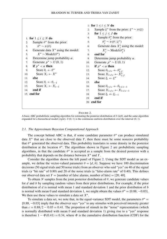
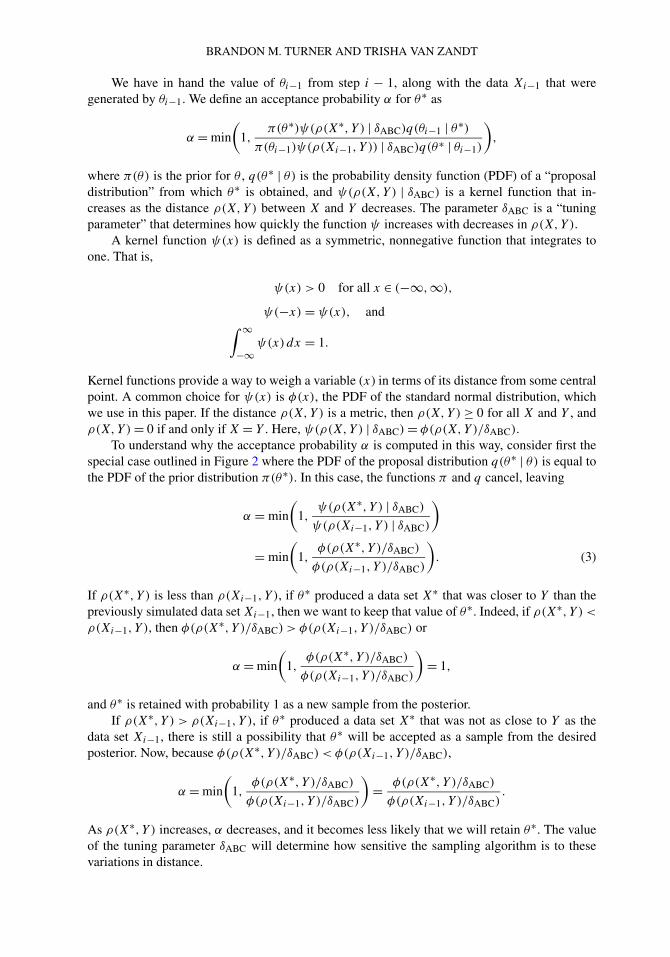
1: for 1 ≤ i ≤ N do2: Sample θ∗ from the prior:3: θ∗ ∼ π(θ)
4: Generate data X∗ using the model:5: X∗ ∼ Model(θ∗)6: Determine jump probability α.7: Generate p∗ ∼ U(0,1)
8: if p∗ < α then9: Store θi ← θ∗
10: Store Xi ← X∗11: else12: Store θi ← θi−113: Store Xi ← Xi−114: end if15: end for
1: for 1 ≤ i ≤ N do2: Sample ξ∗ from the prior: ξ∗ ∼ π(ξ)
3: for 1 ≤ j ≤ J do4: Sample θ∗
j from the prior:5: θ∗
j ∼ π(θ | ξ∗)6: Generate data X∗
j using the model:7: X∗
j ∼ Model(θ∗j )
8: end for9: Determine jump probability α.
10: Generate p∗ ∼ U(0,1)
11: if p∗ < α then12: Store θ1:J,i ← θ∗
1:J13: Store X1:J,i ← X∗
1:J14: Store ξi ← ξ∗15: else16: Store θ1:J,i ← θ1:J,i−117: Store X1:J,i ← X1:J,i−118: Store ξi ← ξi−119: end if20: end for
FIGURE 2.A basic ABC probabilistic sampling algorithm for estimating the posterior distribution of θ (left), and the same algorithmexpanded for a hierarchical model (right). U(0,1) is the continuous uniform distribution over the interval (0,1).
2.1. The Approximate Bayesian Computational Approach
The concept behind ABC is that, if some candidate parameter θ∗ can produce simulateddata X∗ that are close to the observed data Y , then there must be some nonzero probabilitythat θ∗ generated the observed data. This probability translates to some density in the posteriordistribution at the location θ∗. The algorithms shown in Figure 2 are probabilistic samplingalgorithms, in that the candidate θ∗ is accepted as a sample from the desired posterior with aprobability that depends on the distance between X∗ and Y .
Consider the algorithm shown the left panel of Figure 2. Using the SDT model as an ex-ample, we define the vector-valued parameter θ = {d, b}. Suppose we have 100 discriminationdecisions (50 signal trials and 50 noise trials) from an observer who said “yes” on 40 of the signaltrials (a “hit rate” of 0.80) and 20 of the noise trials (a “false-alarm rate” of 0.40). This definesour observed data set Y = {number of false alarms, number of hits} = {20,40}.
To obtain N samples from the joint posterior distribution of θ , we generate candidate valuesfor d and b by sampling random values from their prior distributions. For example, if the priordistribution of d is normal with mean 1 and standard deviation 1 and the prior distribution of b
is normal with mean 0 and standard deviation 1, we might obtain the values θ∗ = {0.88,−0.03}.We then use these values to simulate a data set X∗.
To simulate a data set, we note that, in the equal-variance SDT model, the parameters θ∗ ={0.88,−0.03} imply that the observer says “yes” to any stimulus with perceived intensity greaterthan c = 0.88/2 − 0.03 = 0.41. The proportion of stimuli in the “noise” representation (whichis normally distributed with mean 0 and standard deviation 1) giving rise to a “yes” responseis therefore 1 − Φ(0.41) = 0.34, where Φ is the cumulative distribution function (CDF) for the
PSYCHOMETRIKA
standard normal distribution. Similarly, the proportion of stimuli in the “signal” representation(which is normally distributed with mean 0.88 and standard deviation 1) giving rise to a “yes”response is therefore 1−Φ(0.41−0.88) = 0.68. We can then generate a sample from a binomialdistribution with number of trials equal to 50 and probability of success equal to 0.34 for thesimulated false alarms, and another sample from a binomial distribution with number of trialsequal to 50 and probability of success equal to 0.68 for the simulated hits.
Using the binomial probabilities 0.34 and 0.68, we might obtain the simulated data set X∗ ={19,30}. We must now determine whether θ∗ has any reasonable chance of having been drawnfrom the desired posterior π(θ | Y). To do that, we must decide how close X∗ is to Y . If X∗ isvery close to Y , we will have a high probability of accepting θ∗, and this probability will decreaseas the distance between X∗ and Y increases.
2.1.1. Defining Distance Between X∗ and Y The success of ABC algorithms hinges onhow we measure the distance ρ(X,Y ) between two data sets X and Y . For our running SDTexample, Y = {number of false alarms, number of hits} = {20,40}. For θ∗ = {0.88,−0.03} wegenerated X∗ = {19,30}. One likely distance function might be the Euclidean metric
ρ(X∗, Y
) = (X∗
1 − Y1)2 + (
X∗2 − Y2
)2 = 101.
If ρ(X,Y ) is chosen well, then ABC algorithms allow us to obtain an approximation tothe posterior distribution π(θ | Y) that is conditioned on the values of the discriminant functionρ(X,Y ) rather than the data Y alone. That is,
π(θ | Y) ≈ π(θ | ρ(X,Y ) ≤ ε
). (2)
This approximation is exact for certain algorithms under the appropriate choice of ρ(X,Y ).Specifically, ρ(X,Y ) should be a function of sufficient summary statistics S(X) and S(Y ).A thorough discussion of this issue is beyond the scope of this paper. Interested readers shouldconsult Turner and Van Zandt (2012) and Wilkinson (2011), and be assured that the algorithmwe present here satisfies the conditions for exact posterior estimates.
The quantity ε is called a tolerance threshold. For many realistic problems, it is unlikely thatwe will be able to generate data X∗ so that ρ(X∗, Y ) = 0, especially if Y and X∗ are continuous,or if the sample size of Y and X∗ is very large. For this reason, some ABC algorithms use afixed tolerance threshold ε such that if ρ(X∗, Y ) ≤ ε we keep θ∗ as a sample of θ from anapproximation of the posterior distribution π(θ | Y). However, if ρ(X∗, Y ) > ε then we discardthe proposed θ∗.
These rejection procedures face two problems. First, if ε is too small, it will be difficult togenerate X∗ close enough to Y to accept θ∗, which means that the rejection rate will be veryhigh and computation time will be greatly increased. Second, if ε is not small enough, thenthe approximation π(θ | ρ(X,Y ) < ε) will not be very good. A number of solutions have beenproposed to ameliorate these problems (see, e.g., Turner & Van Zandt, 2012, for a review), butan alternative is to use kernel-based ABC, a method that smoothly weights the “fitness” of θ∗based on the distance between X∗ and Y (Turner & Sederberg, 2012; Wilkinson, 2011).
2.1.2. Sampling Values of θ Consider whether or not we should accept a proposal θ∗ onstep i of the algorithm shown in the left panel of Figure 2. We described earlier the Metropolis–Hastings method, which is one way of making an accept/reject decision in a MCMC algorithm.The method we describe here is very similar to the standard Metropolis–Hastings method, exceptthat it is based on an evaluation of the distance ρ(X∗, Y ) instead of the posterior probability of θ∗.
BRANDON M. TURNER AND TRISHA VAN ZANDT
We have in hand the value of θi−1 from step i − 1, along with the data Xi−1 that weregenerated by θi−1. We define an acceptance probability α for θ∗ as
α = min
(1,
π(θ∗)ψ(ρ(X∗, Y ) | δABC)q(θi−1 | θ∗)π(θi−1)ψ(ρ(Xi−1, Y )) | δABC)q(θ∗ | θi−1)
),
where π(θ) is the prior for θ , q(θ∗ | θ) is the probability density function (PDF) of a “proposaldistribution” from which θ∗ is obtained, and ψ(ρ(X,Y ) | δABC) is a kernel function that in-creases as the distance ρ(X,Y ) between X and Y decreases. The parameter δABC is a “tuningparameter” that determines how quickly the function ψ increases with decreases in ρ(X,Y ).
A kernel function ψ(x) is defined as a symmetric, nonnegative function that integrates toone. That is,
ψ(x) > 0 for all x ∈ (−∞,∞),
ψ(−x) = ψ(x), and∫ ∞
−∞ψ(x)dx = 1.
Kernel functions provide a way to weigh a variable (x) in terms of its distance from some centralpoint. A common choice for ψ(x) is φ(x), the PDF of the standard normal distribution, whichwe use in this paper. If the distance ρ(X,Y ) is a metric, then ρ(X,Y ) ≥ 0 for all X and Y , andρ(X,Y ) = 0 if and only if X = Y . Here, ψ(ρ(X,Y ) | δABC) = φ(ρ(X,Y )/δABC).
To understand why the acceptance probability α is computed in this way, consider first thespecial case outlined in Figure 2 where the PDF of the proposal distribution q(θ∗ | θ) is equal tothe PDF of the prior distribution π(θ∗). In this case, the functions π and q cancel, leaving
α = min
(1,
ψ(ρ(X∗, Y ) | δABC)
ψ(ρ(Xi−1, Y ) | δABC)
)
= min
(1,
φ(ρ(X∗, Y )/δABC)
φ(ρ(Xi−1, Y )/δABC)
). (3)
If ρ(X∗, Y ) is less than ρ(Xi−1, Y ), if θ∗ produced a data set X∗ that was closer to Y than thepreviously simulated data set Xi−1, then we want to keep that value of θ∗. Indeed, if ρ(X∗, Y ) <
ρ(Xi−1, Y ), then φ(ρ(X∗, Y )/δABC) > φ(ρ(Xi−1, Y )/δABC) or
α = min
(1,
φ(ρ(X∗, Y )/δABC)
φ(ρ(Xi−1, Y )/δABC)
)= 1,
and θ∗ is retained with probability 1 as a new sample from the posterior.If ρ(X∗, Y ) > ρ(Xi−1, Y ), if θ∗ produced a data set X∗ that was not as close to Y as the
data set Xi−1, there is still a possibility that θ∗ will be accepted as a sample from the desiredposterior. Now, because φ(ρ(X∗, Y )/δABC) < φ(ρ(Xi−1, Y )/δABC),
α = min
(1,
φ(ρ(X∗, Y )/δABC)
φ(ρ(Xi−1, Y )/δABC)
)= φ(ρ(X∗, Y )/δABC)
φ(ρ(Xi−1, Y )/δABC).
As ρ(X∗, Y ) increases, α decreases, and it becomes less likely that we will retain θ∗. The valueof the tuning parameter δABC will determine how sensitive the sampling algorithm is to thesevariations in distance.
PSYCHOMETRIKA
Assume for our running example that ρ(Xi−1, Y ) = 12. Setting the tuning parameter δABC =50, we obtain
α = min
(1,
φ(101/50)
φ(12/50)
)≈ 0.13.
We now sample a p∗ between 0 and 1 from a continuous uniform distribution (p∗ ∼ U(0,1)),and if that p∗ is less than 0.13, then we accept θ∗ = {0.88,−0.03} as a sample from the desiredposterior. We would set θi = θ∗, Xi = X∗, and generate a new proposal θ∗ for the i + 1th step.
The dependence of the rejection rate (the number of θ∗s that are proposed and then rejected)on the tuning parameter δABC is evident when we recompute α with a tuning parameter δABC = 5.In this case,
α = min
(1,
φ(101/5)
φ(12/5)
)≈ 0.
It is now virtually impossible (probability less than 10−89) that we would sample a p∗ from aU(0,1) distribution that is less than α, and we would certainly reject θ∗ = {0.88,−0.03} as asample from the desired posterior. Instead, we would set θi = θi−1 and generate a new proposalθ∗ for the i + 1th step. The ABC implementations in this paper used the normal kernel φ(x)
with tuning parameter δABC = 0.01. The parameter δABC was selected based on preliminarysimulation studies where our goal was to select a δABC that achieved accurate posterior estimateswhile maintaining reasonable acceptance rates (i.e., acceptance rates greater than 10 %).
In the right panel of Figure 2, proposals θ∗ are chosen by sampling from the prior π(θ),which is a common practice in the simplest ABC algorithms. While these simple algorithms areappealing, many models are either too complex or the prior for θ is too diffuse, resulting in largerejection rates to obtain values of ρ(X,Y ) that are small enough. In these situations, we cansample instead from a proposal distribution q(θ∗ | θ), which is chosen so that q is in some way“close” to the desired posterior (also see Fearnhead & Prangle, 2012, for more principled rules).If q(θ∗ | θ) is symmetric, so that q(θ∗ | θ) = q(θ | θ∗), then the choice of q(θ∗ | θ) has no effecton the acceptance probability and α can be understood as we described above. In this paper, wechose q(θ∗ | θ) to be the normal distribution with mean θ and standard deviation 0.1, which issymmetric.
2.1.3. Gibbs Sampling Having now considered the dual problems of proposing values forθ and evaluating their fitness, we must now consider the problem of scaling up into higher-dimensional parameter spaces. In our running SDT example, θ = {d, b} is two-dimensional, andit is not very difficult to imagine extending the algorithm in the left panel of Figure 2 to three,four, or even more dimensions. The ability to extend the algorithm will be limited when we beginto tackle the problem of hierarchical models, with the subject-level parameters for each subject,plus the hyperparameters in the upper levels of the hierarchy.
Estimating all the posteriors for the subject- and group-level parameters requires that weobtain a large number of n-dimensional samples from an n-dimensional joint probability distri-bution. Sampling from a joint distribution is more difficult than sampling from the (univariate)distribution of a single variable, but under general conditions, we can use a technique calledGibbs sampling to make this process more tractable.
Consider our SDT experiment with a single subject. We have been writing the subject’sparameters as the vector θ = {d, b}. Although it might be possible, we do not typically try tosample from the joint distribution of {d, b}. Instead, we initialize (perhaps by sampling from thepriors) the sequence of samples (called the chain) to θ1 = {d1, b1}, and then begin a process wherewe select d2 by sampling from the conditional distribution of d | b = b1, and then select b2 bysampling from the conditional distribution of b | d = d2. This process is called Gibbs sampling.
BRANDON M. TURNER AND TRISHA VAN ZANDT
Gibbs sampling requires that we know the conditional posteriors π(b | d,Y ) and π(d | b,Y ).If we know the priors for d and b and the probability of Y given d and b (i.e., the likelihood),then we can either sample directly from the appropriate (known) posteriors or, if the posteriors donot have an obvious analytic form, we can use a convenient MCMC technique, like Metropolis–Hastings or slice sampling. (These are the methods used by the popular Gibbs sampling programWinBUGS; see Lunn, Thomas, Best, & Spiegelhalter, 2000.)
More generally, for a fully hierarchical problem, we might consider a SDT experiment withJ subjects. Each subject’s parameters θj (j = 1, . . . , J ) can be written as the vector θj = {dj , bj }.The model hierarchy assumes that each subject’s dj is sampled from a normal distribution withmean dμ and standard deviation dσ . Similarly, each subject’s bj is sampled from a normal dis-tribution with mean bμ and standard deviation bσ . The group parameters can be written as thevector ξ = {dμ, dσ , bμ, bσ }. We might, for example, specify that the hyperparameter dμ has anormal prior with mean 1 and standard deviation 1, bμ has a normal prior with mean 0 and stan-dard deviation 1, and the hyperparameters dσ and bσ have gamma priors with shape and scaleequal to 1 (i.e., exponential with mean 1).
Our goal is to obtain a large number of samples from the joint distribution of
(ξ, θ) = {dμ, bμ, dσ , bσ , d1, b1, d2, b2, . . . , dJ , bJ },which has dimension KJ + M , where M = 4 is the number of hyperparameters and K = 2 isthe number of subject-specific parameters.
We use θj,k to denote the kth subject-level parameter for Subject j and θj,k,i to denote theith sample of θj,k obtained on iteration i. Similarly, ξm,i is the value of the mth hyperparameterξm on iteration i. We will also write ξ1:M,i and θ1:J,1:K,i to indicate all the values defining thevectors ξ and θ on the ith iteration. Using Gibbs sampling, we obtain samples from the jointposterior by first initializing the values of all the parameters to
ξ1:M,1 = {dμ,1, bμ,1, dσ,1, bσ,1} and
θ1:J,1:K,1 = {d1,1, b1,1, d2,1, b2,1, . . . , dJ,1, bJ,1}.Then, on each iteration i > 1, we obtain samples from the conditional distributions of
ξm | ξ−m, θ, and
θj | θ−j , ξ(4)
for j = 1,2, . . . , J and m = 1,2, . . . ,M , where ξ−m denotes the set of parameters ξ excludingthe mth element, so that
ξ−m = {ξ1, . . . , ξm−1, ξm+1, . . . , ξM}.To do this sampling in the Gibbs framework, we update each set of parameters separately
by setting all of the other parameters to their current value in the chain. Thus, ξm is updated bysetting
θ = θ1:J,1:K,1, and
ξ−m = {ξ1,2, ξ2,2, . . . , ξm−1,2, ξm+1,1, . . . , ξM,1}in Equation (4), and θj is updated by setting
in Equation (4). This is straightforward, if a little tedious, to implement for models with ananalytic likelihood function.
If the model under consideration does not have an analytic likelihood function, then we mustconsider methods to adapt the algorithm in the left panel of Figure 2 to the hierarchical problem.The right panel of Figure 2 shows a naïve solution to this problem in which the hyperparametervector ξ is updated in a single step together with the parameters θ .
The right panel of Figure 2, which does not use Gibbs sampling, breaks the sampling prob-lem into two steps. First, we sample proposal hyperparameters ξ∗ from the prior π(ξ) andthen we sample proposal parameters θ∗
j from the conditional prior π(θj | ξ∗). Writing the dataY = {Y1, Y2, . . . , YJ }, so that Yj represents the observations taken on Subject j , each set of pa-rameters {ξ∗, θ∗
j } must generate data X∗j so that ρ(X∗
j , Yj ) ≤ ε. If a candidate hyperparameterξ∗ produces θ∗
j s that satisfy the criterion for all j ∈ {1,2, . . . , J }, then ξ∗ and the θ∗j s have some
nonzero density in the approximate joint posterior distribution π(ξ, θ | ρ(X,Y ) ≤ ε).2 If it is notpossible to find a θ∗
j that produces X∗j close to Yj , even if all the other θ∗
l �=j produced X∗l s close
to their Yls, then the proposed ξ∗ and all the proposed θ∗j s must be discarded and the search for
a sample of θ begins again with a new ξ∗. Therefore, this algorithm, while producing accurateestimates of the posterior is like the algorithm in the left panel of Figure 2, hopelessly inefficientfor even moderately complex problems.
We could do several things to make the algorithm more efficient. First, we could use anempirical Bayes method. Empirical Bayes methods inform the choice of the priors by first usingclassical estimation techniques such as maximum likelihood. For example, given the maximumlikelihood estimate ξ̂ for ξ , we could generate the θ∗
j s from the conditional prior π(θj | ξ̂ ) (Line 5of the right panel of Figure 2; see Pritchard et al., 1999, for an example). Second, we could allowthe simulated data X∗
j to be arranged in any way possible to optimize the acceptance rate. Thatis, we might not want to restrict our comparison of X∗
j to data Yj ; perhaps data Yl are closer toX∗
j and we could accept θ∗j on that basis (see, e.g., Hickerson, Stahl, & Lessios, 2006; Hickerson
& Meyer, 2008; Sousa, Fritz, Beaumont, & Chikhi, 2009). Finally, Bazin, Dawson, and Beau-mont (2010) proposed a two-stage technique that can improve the naïve sampler. However, thismethod introduces additional error above and beyond the error encountered when ρ(X,Y ) �= 0(Beaumont, 2010).
Gibbs sampling, however, provides a way to avoid the pitfalls of the naïve sampler entirely,and so we now present an alternative method that permits sampling from the posteriors of a fullyhierarchical model with much greater computational efficiency.
2.2. The Gibbs ABC Algorithm
In this section, we show how we can sample directly from the conditional posterior distribu-tion of the hyperparameters using well-accepted techniques. The key insight to this approach isthe fact that the conditional distribution of the hyperparameters does not depend on the likelihoodfunction. This, in combination with a mixture of Gibbs sampling and ABC sampling provides analgorithm that offers a significant improvement in accuracy and computation efficiency.
To implement the algorithm, we first consider the conditional posterior distribution of thesubject-level parameters θ , which is
π(θ | Y, ξ) ∝ L(θ | Y, ξ)π(θ | ξ)
∝J∏
j=1
L(θj | Yj )π(θj | ξ),
2One can also use a kernel to weigh the fitness of the proposals ξ∗ and θ∗j
.
BRANDON M. TURNER AND TRISHA VAN ZANDT
given the conditional independence of the θj s and Yj s. To see that the parameter ξ can be droppedfrom the likelihood, recall that the likelihood for Subject j can be seen as the probability ofthe data Yj given the parameters θj ; there is no role played by ξ in the PDF of Yj , and so thelikelihood Yj depends on ξ only through the parameters θj . The conditional posterior distributionof θj given the data and all of the other parameters is therefore
π(θj | Y, ξ) ∝ L(θj | Yj )π(θj | ξ). (5)
Because the conditional posterior distribution of each of the θj s depends on the partition ofthe data exclusive to the j th subject, the problem simplifies to performing ABC for each subject,and we can approximate each conditional posterior by
π(θj | Y, ξ) ≈ ψ(ρ(Xj ,Y )|δABC
)π(θj | ξ). (6)
Noting that π(ξ | Y, θ) ∝ π(θ | ξ)π(ξ), the joint conditional posterior distribution of thehyperparameters ξ is
π(ξ | Y, θ) ∝ L(θ | Y)π(θ | ξ)π(ξ)
∝ π(θ | ξ)π(ξ)
∝ π(ξ)
J∏
j=1
π(θj | ξ). (7)
Because ξ influences the likelihood only through the parameter θ , the joint conditional distri-bution of ξ = {ξ1, . . . , ξm, . . . , ξM} does not depend on the likelihood; the likelihood is just aconstant with respect to ξ . This means that we can sample from the conditional posterior distri-bution of ξ using standard techniques. If this distribution has a convenient form, we can directlysample from it. Otherwise, we can use any numerical technique, such as discretized sampling(e.g., Gelman et al., 2004), adaptive rejection sampling (Gilks & Wild, 1992), or MCMC (e.g.,Robert & Casella, 2004).
This brings us to the Gibbs ABC algorithm shown in Figure 3, which is a mixture of stan-dard and ABC estimation techniques. After initializing values for ξ1:M,1 and θ1:J,1:K,1, on eachiteration i > 2, we first draw samples of ξm,i conditioned on all other parameters in the model,including all other values in the vector ξ . We use a Gibbs sampler to obtain values of ξ1:M,i bysampling directly from π(ξm | Y, θ1:J,1:K,i−1, ξ−m,i) given by Equation (7).
Having obtained the values for ξ on iteration i, we then use those values to generate samplesfrom the joint conditional posterior distribution of θ using ABC. If the distribution q(θ) fromwhich the proposed values θ∗
j,k are drawn is equal to the prior distribution π(θj,k | θj,−k,i , ξ1:M,i)
then the jumping probability α is calculated in a similar manner as in Equation (3).The Gibbs ABC algorithm is considerably more flexible than other hierarchical ABC algo-
rithms. We can use any appropriate sampling method to estimate the posterior distribution of ξ
and, if necessary, we could use different discriminant functions ρ(X∗, Y ) and tuning parametersδABC for each subject. This might be useful when the model is misspecified, and so allowing forlarge distances for some subjects could improve convergence speed.
Consider, for example, a model that predicts a positive relationship between variables butthe j th subject shows a negative relationship. In this situation, there will be no values for θ∗
j thatcould simulate data X∗
j close to the observed data Yj . Only by increasing δABC will ρ(X∗j , Yj )
be given a weight high enough that θ∗j has a reasonable chance of being accepted.3
3Note that the posterior distributions of θ and ξ will still exist despite a misspecified model. The goal is to estimatethe shapes of those posteriors by generating data that is close to the observed data as measured by ρ(Xj ,Yj ).
PSYCHOMETRIKA
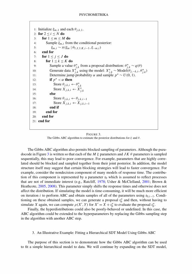
1: Initialize ξm,1 and each θj,k,1.2: for 2 ≤ i ≤ N do3: for 1 ≤ m ≤ M do4: Sample ξm,i from the conditional posterior:5: ξm,i ∼ π(ξm | θ1:J,1:K,i−1, ξ−m,i)
6: end for7: for 1 ≤ j ≤ J do8: for 1 ≤ k ≤ K do9: Sample a value θ∗
j,k from a proposal distribution: θ∗j,k ∼ q(θ)
10: Generate data X∗j,k using the model: X∗
j,k ∼ Model(θj,−k,i , θ∗j,k)
11: Determine jump probability α and sample p∗ ∼ U(0,1).12: if p∗ < α then13: Store θj,k,i ← θ∗
j,k
14: Store Xj,k,i ← X∗j,k
15: else16: Store θj,k,i ← θj,k,i−117: Store Xj,k,i ← Xj,k,i−118: end if19: end for20: end for21: end for
FIGURE 3.The Gibbs ABC algorithm to estimate the posterior distributions for ξ and θ .
The Gibbs ABC algorithm also permits blocked sampling of parameters. Although the pseu-docode in Figure 3 is written so that each of the M ξ parameters and JK θ parameters is sampledsequentially, this may lead to poor convergence. For example, parameters that are highly corre-lated should be blocked and sampled together from their joint posterior. In addition, the modelstructure itself may suggest that certain blocking strategies will lead to faster convergence. Forexample, consider the nondecision component of many models of response time. The contribu-tion of this component is represented by a parameter t0 which is assumed to reflect processesthat are not of immediate interest (e.g., Ratcliff, 1978; Usher & McClelland, 2001; Brown &Heathcote, 2005, 2008). This parameter simply shifts the response times and otherwise does notaffect the distribution. If simulating the model is time-consuming, it will be much more efficienton iteration i to perform ABC and obtain samples of all of the parameters using t0,i−1. Condi-tioning on these obtained samples, we can generate a proposal t∗0 and then, without having tosimulate X again, we can compute ρ(X′, Y ) for X′ = X + t∗0 to evaluate the proposal t∗0 .
Finally, the hyperdistributions could also be poorly-behaved or undefined. In this case, theABC algorithm could be extended to the hyperparameters by replacing the Gibbs sampling stepin the algorithm with another ABC step.
3. An Illustrative Example: Fitting a Hierarchical SDT Model Using Gibbs ABC
The purpose of this section is to demonstrate how the Gibbs ABC algorithm can be usedto fit a simple hierarchical model to data. We will continue by expanding on the SDT model,
BRANDON M. TURNER AND TRISHA VAN ZANDT
adding hyperparameters that describe the distributions from which the subject-level SDT pa-rameters were sampled. Because this model has an analytic likelihood function, we can contrastthe estimated posteriors obtained using Gibbs ABC with those obtained using standard MCMCmethods. We will show that the posteriors estimated in these two ways are very similar, and soargue that Gibbs ABC can be very accurate.
3.1. The Model
Each subject’s probability of a “yes” response is determined by a discriminability parameterdj and a bias parameter bj . The discriminability parameters dj follow a normal distribution withmean dμ and standard deviation dσ , and the bias parameters bj follow a normal distributionwith mean bμ and standard deviation bσ . The mean hyperparameter dμ has a normal prior withmean 1 and standard deviation 1, and the hyperparameter bμ has a normal prior with mean 0and standard deviation 1. The standard deviation hyperparameters dσ and bσ have gamma priorswith shape and scale equal to 1.4
We simulated the model by first setting dμ = 1, bμ = 0, dσ = 0.20, and bσ = 0.05. Usingthese parameter values, we drew a dj and bj for each of nine subjects from the normal hyperdis-tributions. We then used these subject-level parameters to generate “yes” responses for noise andsignal trials by sampling from binomial distributions with probabilities equal to the areas underthe normal curves to the right of dj /2 + bj and N equal to 500.
3.2. Results
To apply the Gibbs ABC algorithm to the “observed” (simulated) data, we set ρ(X,Y ) equalto the Euclidean distance between the observed and simulated (using proposed values for θ ) vec-tors of hit and false alarm rates. This distance was weighed with a Gaussian kernel using a tuningparameter δABC = 0.01. We generated 24 independent chains of 10,000 draws of each parameter,discarding the first 1,000 iterations chain as a “burn-in” period. We did not thin the chains, andso we obtained 216,000 samples to form an estimate of the joint posterior distributions for eachparameter.
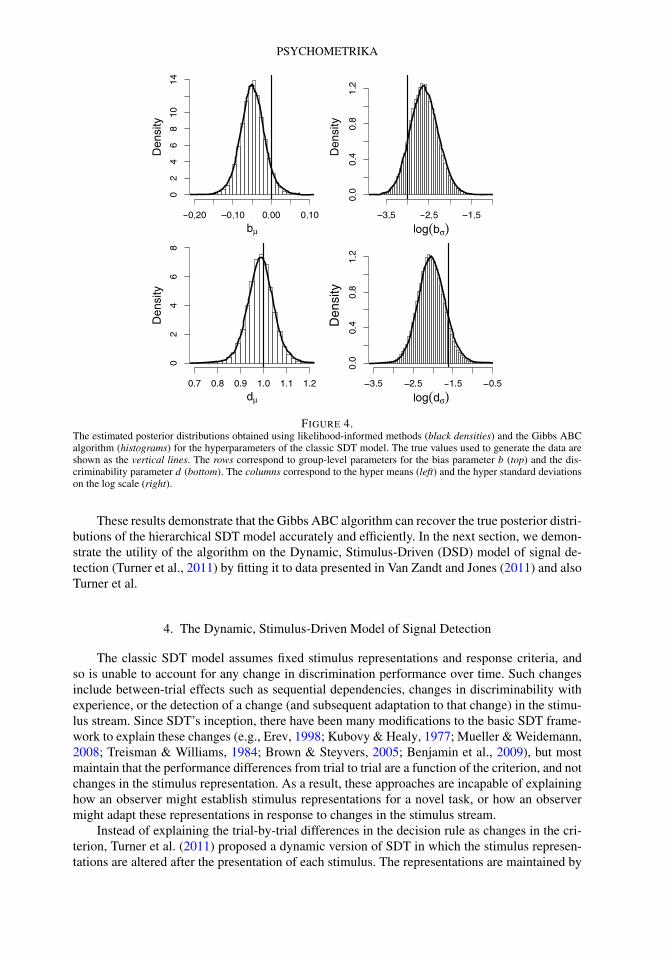
Figure 4 shows the estimated posterior distributions for the model’s hyperparameters (dμ,bμ, dσ , and bσ ) as histograms plotted behind solid lines. These lines are the posterior densityestimates obtained using a likelihood-informed method (MCMC), and the vertical lines representthe true values of the hyperparameters. The left panel of Figure 4 shows these estimates for thehyper mean parameters for the bias parameter bμ (top) and the discriminability parameter dμ
(bottom). The right panel shows the estimates for the hyper standard deviation parameters forthe bias parameter bσ (top) and the discriminability parameter dσ (bottom) on the log scale. Theestimates obtained using our Gibbs ABC algorithm closely match the estimates obtained usingconventional MCMC.
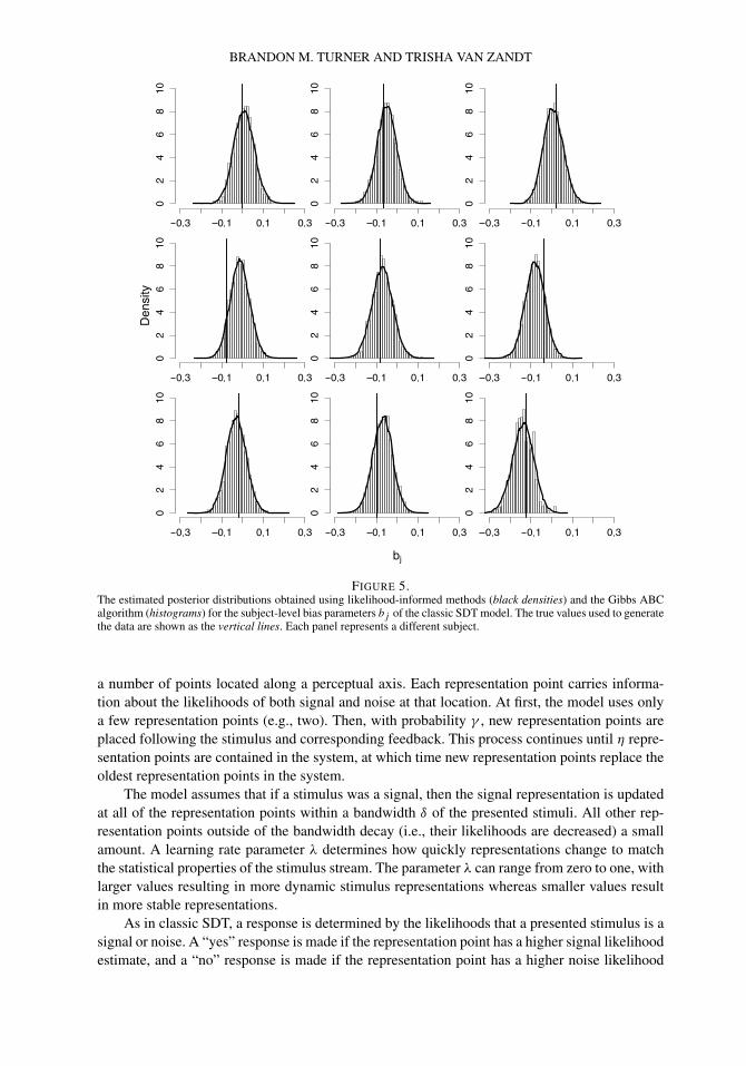
While Figure 4 shows that the estimates using Gibbs ABC and likelihood-informed MCMCmethods match closely at the group level, it is also important to show that the Gibbs ABC al-gorithm provides estimates that closely match standard MCMC methods at the subject level.Figures 5 and 6 show the estimated posterior distributions for the bias (bj ) and discriminability(dj ) parameters, respectively, for each of the nine subjects. The vertical dashed lines in eachpanel show the values used to generate the data. Together, the figures show that the Gibbs ABCalgorithm also provides accurate estimates at the subject level.
4We investigated a range of priors and determined that the choice of priors, if reasonably variable, had little effecton the final estimated posterior. The priors that we selected permit a range of values for d and b that reflect those that arereported in the perceptual and memory literature (Rouder & Lu, 2005; Lee, 2008).
PSYCHOMETRIKA
FIGURE 4.The estimated posterior distributions obtained using likelihood-informed methods (black densities) and the Gibbs ABCalgorithm (histograms) for the hyperparameters of the classic SDT model. The true values used to generate the data areshown as the vertical lines. The rows correspond to group-level parameters for the bias parameter b (top) and the dis-criminability parameter d (bottom). The columns correspond to the hyper means (left) and the hyper standard deviationson the log scale (right).
These results demonstrate that the Gibbs ABC algorithm can recover the true posterior distri-butions of the hierarchical SDT model accurately and efficiently. In the next section, we demon-strate the utility of the algorithm on the Dynamic, Stimulus-Driven (DSD) model of signal de-tection (Turner et al., 2011) by fitting it to data presented in Van Zandt and Jones (2011) and alsoTurner et al.
4. The Dynamic, Stimulus-Driven Model of Signal Detection
The classic SDT model assumes fixed stimulus representations and response criteria, andso is unable to account for any change in discrimination performance over time. Such changesinclude between-trial effects such as sequential dependencies, changes in discriminability withexperience, or the detection of a change (and subsequent adaptation to that change) in the stimu-lus stream. Since SDT’s inception, there have been many modifications to the basic SDT frame-work to explain these changes (e.g., Erev, 1998; Kubovy & Healy, 1977; Mueller & Weidemann,2008; Treisman & Williams, 1984; Brown & Steyvers, 2005; Benjamin et al., 2009), but mostmaintain that the performance differences from trial to trial are a function of the criterion, and notchanges in the stimulus representation. As a result, these approaches are incapable of explaininghow an observer might establish stimulus representations for a novel task, or how an observermight adapt these representations in response to changes in the stimulus stream.
Instead of explaining the trial-by-trial differences in the decision rule as changes in the cri-terion, Turner et al. (2011) proposed a dynamic version of SDT in which the stimulus represen-tations are altered after the presentation of each stimulus. The representations are maintained by
BRANDON M. TURNER AND TRISHA VAN ZANDT
FIGURE 5.The estimated posterior distributions obtained using likelihood-informed methods (black densities) and the Gibbs ABCalgorithm (histograms) for the subject-level bias parameters bj of the classic SDT model. The true values used to generatethe data are shown as the vertical lines. Each panel represents a different subject.
a number of points located along a perceptual axis. Each representation point carries informa-tion about the likelihoods of both signal and noise at that location. At first, the model uses onlya few representation points (e.g., two). Then, with probability γ , new representation points areplaced following the stimulus and corresponding feedback. This process continues until η repre-sentation points are contained in the system, at which time new representation points replace theoldest representation points in the system.
The model assumes that if a stimulus was a signal, then the signal representation is updatedat all of the representation points within a bandwidth δ of the presented stimuli. All other rep-resentation points outside of the bandwidth decay (i.e., their likelihoods are decreased) a smallamount. A learning rate parameter λ determines how quickly representations change to matchthe statistical properties of the stimulus stream. The parameter λ can range from zero to one, withlarger values resulting in more dynamic stimulus representations whereas smaller values resultin more stable representations.
As in classic SDT, a response is determined by the likelihoods that a presented stimulus is asignal or noise. A “yes” response is made if the representation point has a higher signal likelihoodestimate, and a “no” response is made if the representation point has a higher noise likelihood
PSYCHOMETRIKA
FIGURE 6.The estimated posterior distributions obtained using likelihood-informed methods (black densities) and the Gibbs ABCalgorithm (histograms) for the subject-level discriminability parameters dj of the classic SDT model. The true valuesused to generate the data are shown as the vertical lines. Each panel represents a different subject.
FIGURE 7.An example of how the DSD model evolves the representations (dotted lines) for both signal (black) and noise (gray)to match the true stimulus-generating distributions (solid lines). The top, middle, and bottom panels show the DSDTmodel’s representations after 5, 50, and 100 trials.
BRANDON M. TURNER AND TRISHA VAN ZANDT
estimate, or if the two likelihoods are equal, a guess is made by choosing either the “yes” or “no”response with equal probabilities.
Figure 7 shows how the representations produced by the DSD model change over time.The dotted lines represent the noise (gray) and signal (black) representations used by the model,and each dot corresponds to a representation point. At first, the model uses only a few points(top panel), but after the model is presented with more stimuli, the representations begin to lookmore like the true stimulus-generating distributions (solid lines). Finally, after many stimuluspresentations, the representations closely resemble the true stimulus generating distribution, asshown in the bottom panel.
Turner et al. (2011) showed how the dynamic updating process was a useful extension of thebasic SDT framework. However, the dynamic representations, which change from trial to trial,makes generating model predictions difficult. To compute the probability of a “yes” response onTrial t , one would first need to know the probabilities of the different possible representations onTrial t , which would depend on the stimuli presented on Trials 1 to t −1, as well as the responsesto them. The derivation of these probabilities is a very difficult problem, and to avoid it, Turneret al. resorted to hand-held fits obtained by approximate least-squares.
Hand-held fitting procedures severely limit the extent to which inference can be made abouta model’s parameters. In particular, one cannot assess how one subject differs from another andhow that subject’s performance might differ from the group of subjects in the experiment. TheHABC approach allows for full hierarchical Bayesian inference despite the lack of explicit ex-pressions for a model’s likelihood. We now use Gibbs ABC to fit the DSD model to the data fromTurner et al. (2011).
4.1. The Model
We used the data from the low d ′ condition of Experiment 1 reported in Turner et al. (2011).In this experiment, subjects were presented with 340 patient blood assays and asked to determinewhether the patient had been infected with a deadly disease or not. If a subject indicated thatthe patient had been infected (by means of a “yes” response) then that patient would receivetreatment for the disease. However, subjects were told that healthy (i.e., uninfected) patients whoreceived treatment would die as a consequence of the treatment. By contrast, if a subject indicatedthat a patient did not have the disease (by means of a “no” response) then that patient would notreceive treatment. If a sick patient (i.e., an infected patient) was not treated, that patient woulddie as a consequence of the disease.
The blood assays were presented in the form of numbers randomly drawn from Gaussiandistributions with means of 40 and 60 for healthy and sick patients, respectively, and with com-mon standard deviations of 10. The 340 blood assays were completed over 5 blocks of 68 trialseach, for 31 subjects. Additional experimental details can be found in Turner et al. (2011) andVan Zandt and Jones (2011).
Our goal is to make inferences about each of the model parameters for each subject indi-vidually while simultaneously making inferences about the group-level parameters. The param-eters of interest are: γ , the probability of adding/replacing a representation point; λ, the learningrate; δ, the bandwidth; and η, the maximum number of representation points. The j th subject’sparameters are γj , λj , δj , and ηj . We specified a hyperdistribution from which each of thesesubject-level parameters were drawn, and the hyperparameters (e.g., the mean and variance) of
PSYCHOMETRIKA
each hyperdistribution formed the basis of our group-level analysis. For this model, we set
γj ∼ T N (γμ, γσ ,0,1),
λj ∼ T N (λμ,λσ ,0,1),
δj ∼ T N (δμ, δσ ,0,∞), and
ηj ∼ T N (ημ,ησ ,2,∞),
where T N (s, t, u, v) denotes a truncated normal distribution with mean parameter s, standarddeviation parameter t , lower bound u and upper bound v. The truncated normal distribution is aconvenient choice for defining boundaries for the space of each subject parameter. For example,δ cannot go below zero, and we suspected that the variability between parameter values for eachsubject would be approximately normally distributed. For η, we chose a lower bound of two toforce the model to maintain at least two representation points for each subject.
To complete the hierarchical Bayesian model, we specified mildly informative priors foreach of the hypermeans, such that
γμ ∼ Beta(1,1),
λμ ∼ Beta(1,1),
δμ ∼ T N (10,5,0,∞), and
ημ ∼ T N (20,10,2,∞),
and hyper standard deviations, such that
γσ ∼ Γ (1,1),
λσ ∼ Γ (1,1),
δσ ∼ Γ (5,1), and
ησ ∼ Γ (5,1).
Because we have never fit the DSD model in a Bayesian framework, we had little guidance inselecting the priors. As such, we specified priors to be consistent with the parameter estimatesobtained in Turner et al. (2011), but we maintained a great deal of uncertainty to reflect ourinexperience with the model’s parameters.
4.2. Results
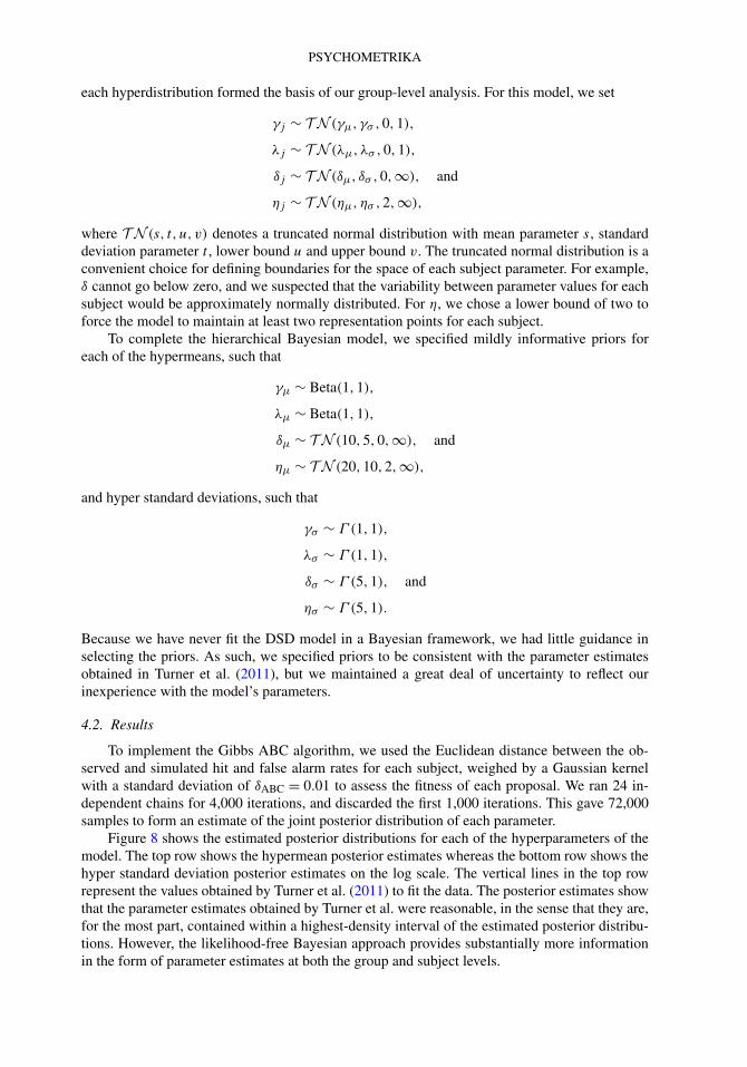
To implement the Gibbs ABC algorithm, we used the Euclidean distance between the ob-served and simulated hit and false alarm rates for each subject, weighed by a Gaussian kernelwith a standard deviation of δABC = 0.01 to assess the fitness of each proposal. We ran 24 in-dependent chains for 4,000 iterations, and discarded the first 1,000 iterations. This gave 72,000samples to form an estimate of the joint posterior distribution of each parameter.
Figure 8 shows the estimated posterior distributions for each of the hyperparameters of themodel. The top row shows the hypermean posterior estimates whereas the bottom row shows thehyper standard deviation posterior estimates on the log scale. The vertical lines in the top rowrepresent the values obtained by Turner et al. (2011) to fit the data. The posterior estimates showthat the parameter estimates obtained by Turner et al. were reasonable, in the sense that they are,for the most part, contained within a highest-density interval of the estimated posterior distribu-tions. However, the likelihood-free Bayesian approach provides substantially more informationin the form of parameter estimates at both the group and subject levels.
BRANDON M. TURNER AND TRISHA VAN ZANDT
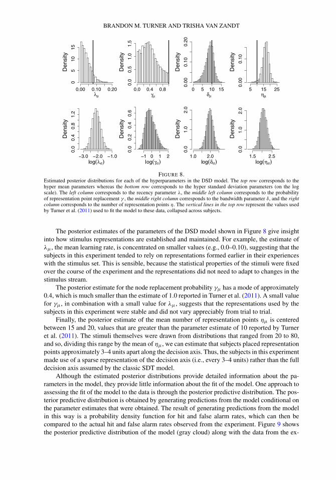
FIGURE 8.Estimated posterior distributions for each of the hyperparameters in the DSD model. The top row corresponds to thehyper mean parameters whereas the bottom row corresponds to the hyper standard deviation parameters (on the logscale). The left column corresponds to the recency parameter λ, the middle left column corresponds to the probabilityof representation point replacement γ , the middle right column corresponds to the bandwidth parameter δ, and the rightcolumn corresponds to the number of representation points η. The vertical lines in the top row represent the values usedby Turner et al. (2011) used to fit the model to these data, collapsed across subjects.
The posterior estimates of the parameters of the DSD model shown in Figure 8 give insightinto how stimulus representations are established and maintained. For example, the estimate ofλμ, the mean learning rate, is concentrated on smaller values (e.g., 0.0–0.10), suggesting that thesubjects in this experiment tended to rely on representations formed earlier in their experienceswith the stimulus set. This is sensible, because the statistical properties of the stimuli were fixedover the course of the experiment and the representations did not need to adapt to changes in thestimulus stream.
The posterior estimate for the node replacement probability γμ has a mode of approximately0.4, which is much smaller than the estimate of 1.0 reported in Turner et al. (2011). A small valuefor γμ, in combination with a small value for λμ, suggests that the representations used by thesubjects in this experiment were stable and did not vary appreciably from trial to trial.
Finally, the posterior estimate of the mean number of representation points ημ is centeredbetween 15 and 20, values that are greater than the parameter estimate of 10 reported by Turneret al. (2011). The stimuli themselves were drawn from distributions that ranged from 20 to 80,and so, dividing this range by the mean of ημ, we can estimate that subjects placed representationpoints approximately 3–4 units apart along the decision axis. Thus, the subjects in this experimentmade use of a sparse representation of the decision axis (i.e., every 3–4 units) rather than the fulldecision axis assumed by the classic SDT model.
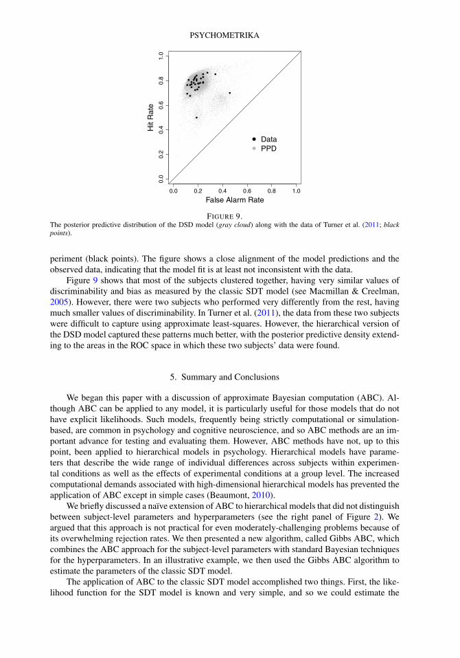
Although the estimated posterior distributions provide detailed information about the pa-rameters in the model, they provide little information about the fit of the model. One approach toassessing the fit of the model to the data is through the posterior predictive distribution. The pos-terior predictive distribution is obtained by generating predictions from the model conditional onthe parameter estimates that were obtained. The result of generating predictions from the modelin this way is a probability density function for hit and false alarm rates, which can then becompared to the actual hit and false alarm rates observed from the experiment. Figure 9 showsthe posterior predictive distribution of the model (gray cloud) along with the data from the ex-
PSYCHOMETRIKA
FIGURE 9.The posterior predictive distribution of the DSD model (gray cloud) along with the data of Turner et al. (2011; blackpoints).
periment (black points). The figure shows a close alignment of the model predictions and theobserved data, indicating that the model fit is at least not inconsistent with the data.
Figure 9 shows that most of the subjects clustered together, having very similar values ofdiscriminability and bias as measured by the classic SDT model (see Macmillan & Creelman,2005). However, there were two subjects who performed very differently from the rest, havingmuch smaller values of discriminability. In Turner et al. (2011), the data from these two subjectswere difficult to capture using approximate least-squares. However, the hierarchical version ofthe DSD model captured these patterns much better, with the posterior predictive density extend-ing to the areas in the ROC space in which these two subjects’ data were found.
5. Summary and Conclusions
We began this paper with a discussion of approximate Bayesian computation (ABC). Al-though ABC can be applied to any model, it is particularly useful for those models that do nothave explicit likelihoods. Such models, frequently being strictly computational or simulation-based, are common in psychology and cognitive neuroscience, and so ABC methods are an im-portant advance for testing and evaluating them. However, ABC methods have not, up to thispoint, been applied to hierarchical models in psychology. Hierarchical models have parame-ters that describe the wide range of individual differences across subjects within experimen-tal conditions as well as the effects of experimental conditions at a group level. The increasedcomputational demands associated with high-dimensional hierarchical models has prevented theapplication of ABC except in simple cases (Beaumont, 2010).
We briefly discussed a naïve extension of ABC to hierarchical models that did not distinguishbetween subject-level parameters and hyperparameters (see the right panel of Figure 2). Weargued that this approach is not practical for even moderately-challenging problems because ofits overwhelming rejection rates. We then presented a new algorithm, called Gibbs ABC, whichcombines the ABC approach for the subject-level parameters with standard Bayesian techniquesfor the hyperparameters. In an illustrative example, we then used the Gibbs ABC algorithm toestimate the parameters of the classic SDT model.
The application of ABC to the classic SDT model accomplished two things. First, the like-lihood function for the SDT model is known and very simple, and so we could estimate the
BRANDON M. TURNER AND TRISHA VAN ZANDT
true posterior distributions easily with standard MCMC techniques. The estimates under MCMCwere very similar to the estimates we obtained using Gibbs ABC for both the group- and subject-level parameters. Therefore, we can conclude that the ABC estimates were accurate. Second,this exercise demonstrates that ABC is not restricted to simulation-based models. The likelihoodof the SDT model, the binomial, is of a simple closed form, and so lends itself well to MCMCmethods (Rouder & Lu, 2005; Lee, 2008). The efficiency of the two methods, ABC and MCMC,was comparable; each fit was obtained in less than 10 minutes.
After this demonstration, we used Gibbs ABC to estimate the parameters of the dynamic,stimulus driven (DSD) model of signal detection. Unlike the classic SDT model, the DSD modelconstructs evolving representations of the two stimulus classes, and the changes in the represen-tations from trial to trial result in an intractable likelihood function. As a result, previous esti-mation of the model parameters was limited to approximate least-squares (Turner et al., 2011)on a restricted version of the full model. Using ABC, we easily fit a complex, hierarchical ver-sion of the full DSD model containing 132 parameters. We were then able to use the parameterestimates we obtained to gain better insight into our model as well as the representations thatsubjects may have used during the experiment. We assessed the model fit by plotting the pre-dictions of the fitted model against the data that were observed. We concluded that the GibbsABC approach provided reasonably accurate posterior estimates because the model predictionsmatched the location and spread of the observed data.
We should note that the DSD model lacks a likelihood only at the subject level. The subject-level parameters were drawn from simple, well-known hyperdistributions. This need not be thecase: the subject-level parameters themselves may have poorly-behaved hyperdistributions. Inthis case, the ABC algorithm could be extended to the hyperparameters.
In previous efforts, we have shown that the ABC approach accurately recovers the posteriordistribution for different models of varying complexity (Turner & Van Zandt, 2012; Turner &Sederberg, 2012). However, these previous applications have been limited because they wereeither not hierarchical or very inefficient. We have shown that the Gibbs ABC algorithm allowsfor accurate estimation of hierarchical model parameters without the use of a likelihood function.As such, the present paper marks an advance toward a fully-Bayesian analysis of hierarchicalsimulation-based models.
References
Bazin, E., Dawson, K.J., & Beaumont, M.A. (2010). Likelihood-free inference of population structure and local adapta-tion in a Bayesian hierarchical model. Genetics, 185, 587–602.
Beaumont, M.A. (2010). Approximate Bayesian computation in evolution and ecology. Annual Review of Ecology, Evo-lution, and Systematics, 41, 379–406.
Benjamin, A.S., Diaz, M., & Wee, S. (2009). Signal detection with criterior noise: applications to recognition memory.Psychological Review, 116, 84–115.
Brown, S., & Heathcote, A. (2005). A ballistic model of choice response time. Psychological Review, 112, 117–128.Brown, S., & Heathcote, A. (2008). The simplest complete model of choice reaction time: linear ballistic accumulation.
Cognitive Psychology, 57, 153–178.Brown, S., & Steyvers, M. (2005). The dynamics of experimentally induced criterion shifts. Journal of Experimental
Psychology. Learning, Memory, and Cognition, 31, 587–599.Christensen, R., Johnson, W., Branscum, A., & Hanson, T.E. (2011). Bayesian ideas and data analysis: an introduction
for scientists and statisticians. Boca Raton: CRC Press, Taylor and Francis Group.DeCarlo, L.T. (2012). On a signal detection approach to m-alternative forced choice with bias, with maximum likelihood
and Bayesian approaches to estimation. Journal of Mathematical Psychology, 56, 196–207.Dennis, S., & Humphreys, M.S. (2001). A context noise model of episodic word recognition. Psychological Review, 108,
452–478.Dorfman, D.D., & Alf, E. (1969). Maximum-likelihood estimation of parameters of signal-detection theory and determi-
nation of confidence intervals—rating-method data. Journal of Mathematical Psychology, 6, 487–496.Efron, B. (1986). Why isn’t everyone a Bayesian? American Statistician, 40, 1–11.Egan, J.P. (1958). Recognition memory and the operating characteristic (Tech. Rep. AFCRC-TN-58-51). Hearing and
Communication Laboratory, Indiana University, Bloomington, Indiana.
PSYCHOMETRIKA
Erev, I. (1998). Signal detection by human observers: a cutoff reinforcement learning model of categoriation decisionsunder uncertainty. Psychological Review, 105, 280–298.
Excoffer, L., Estoup, A., & Cornuet, J.-M. (2005). Bayesian analysis of an admixture model with mutations and arbitrarilylinked markers. Genetics, 169, 1727–1738.
Fearnhead, P., & Prangle, D. (2012). Constructing summary statistics for approximate Bayesian computation: semi-automatic approximate Bayesian computation. Journal of the Royal Statistical Society. Series B, 74, 419–474.
Gelman, A., Carlin, J.B., Stern, H.S., & Rubin, D.B. (2004). Bayesian data analysis. New York: Chapman and Hall.Gilks, W.R., & Wild, P. (1992). Adaptive rejection sampling for Gibbs sampling. Applied Statistics, 41, 337–348.Green, D.M., & Swets, J.A. (1966). Signal detection theory and psychophysics. New York: Wiley.Hickerson, M.J., & Meyer, C. (2008). Testing comparative phylogeographic models of marine vicariance and dispersal
using a hierarchical Bayesian approach. BMC Evolutionary Biology, 8, 322.Hickerson, M.J., Stahl, E.A., & Lessios, H.A. (2006). Test for simultaneous divergence using approximate Bayesian
Journal of Experimental and Theoretical Artificial Intelligence, 20, 197–218.Kubovy, M., & Healy, A.F. (1977). The decision rule in probabilistic categorization: what it is and how it is learned.
Journal of Experimental Psychology. General, 106, 427–446.Lee, M.D. (2008). Three case studies in the Bayesian analysis of cognitive models. Psychonomic Bulletin & Review, 15,
1–15.Lee, M. D., & Wagenmakers, E.-J. (2012). A course in Bayesian graphical modeling for cognitive science. Available
from http://www.ejwagenmakers.com/BayesCourse/BayesBookWeb.pdf; last downloaded January 1, 2012.Lunn, D., Thomas, A., Best, N., & Spiegelhalter, D. (2000). WinBUGS—a Bayesian modelling framework: concepts,
structure and extensibility. Statistics and Computing, 10, 325–337.Macmillan, N.A., & Creelman, C.D. (2005). Detection theory: a user’s guide. Mahwah: Lawrence Erlbaum Associates.Malmberg, K.J., Zeelenberg, R., & Shiffrin, R. (2004). Turning up the noise or turning down the volume? On the nature
of the impairment of episodic recognition memory by Midazolam. Journal of Experimental Psychology. Learning,Memory, and Cognition, 30, 540–549.
Matzke, D., & Wagenmakers, E.-J. (2009). Psychological interpretation of the ex-Gaussian and shifted Wald parameters:a diffusion model analysis. Psychonomic Bulletin & Review, 16, 798–817.
Mazurek, M.E., Roitman, J.D., Ditterich, J., & Shadlen, M.N. (2003). A role for neural integrators in perceptual decisionmaking. Cerebral Cortex, 13, 1257–1269.
McElree, B., & Dosher, B.A. (1993). Serial retrieval processes in the recovery of order information. Journal of Experi-mental Psychology. General, 122, 291–315.
Mueller, S.T., & Weidemann, C.T. (2008). Decision noise: an explanation for observed violations of signal detectiontheory. Psychonomic Bulletin & Review, 15, 465–494.
Myung, I.J. (2003). Tutorial on maximum likelihood estimation. Journal of Mathematical Psychology, 47, 90–100.Nelder, J.A., & Mead, R. (1965). A simplex method for function minimization. Computer Journal, 7, 308–313.Nosofsky, R.M., Little, D.R., Donkin, C., & Fific, M. (2011). Short-term memory scanning viewed as exemplar-based
categorization. Psychological Review, 118, 280–315.Nosofsky, R.M., & Palmeri, T. (1997). Comparing exemplar-retrieval and decision-bound models of speeded perceptual
classification. Perception and Psychophysics, 59, 1027–1048.O’Reilly, R., & Frank, M. (2006). Making working memory work: a computational model of learning in the prefrontal
cortex and basal ganglia. Neural Computation, 18, 283–328.Pritchard, J.K., Seielstad, M.T., Perez-Lezaun, A., & Feldman, M.W. (1999). Population growth of human Y chromo-
somes: a study of Y chromosome microsatellites. Molecular Biology and Evolution, 16, 1791–1798.Ratcliff, R. (1978). A theory of memory retrieval. Psychological Review, 85, 59–108.Ratcliff, R., & Rouder, J.N. (1998). Modeling response times for two-choice decisions. Psychological Science, 9, 347–
356.Ratcliff, R., & Smith, P.L. (2004). A comparison of sequential sampling models for two-choice reaction time. Psycho-
logical Review, 111, 333–367.Ratcliff, R., & Starns, J. (2009). Modeling confidence and response time in recognition memory. Psychological Review,
116, 59–83.Robert, C.P., & Casella, G. (2004). Monte Carlo statistical methods. New York: Springer.Rouder, J.N., & Lu, J. (2005). An introduction to Bayesian hierarchical models with an application in the theory of signal
detection. Psychonomic Bulletin & Review, 12, 573–604.Rouder, J.N., Lu, J., Speckman, P., Sun, D., & Jiang, Y. (2005). A hierarchical model for estimating response time
distributions. Psychonomic Bulletin & Review, 12, 195–223.Rouder, J.N., Sun, D., Speckman, P., Lu, J., & Zhou, D. (2003). A hierarchical Bayesian statistical framework for re-
sponse time distributions. Psychometrika, 68, 589–606.Shiffrin, R.M., Lee, M.D., Kim, W., & Wagenmakers, E.-J. (2008). A survey of model evaluation approaches with a
tutorial on hierarchical Bayesian methods. Cognitive Science, 32, 1248–1284.Shiffrin, R.M., & Steyvers, M. (1997). A model for recognition memory: REM—retrieving effectively from memory.
Psychonomic Bulletin & Review, 4, 145–166.Sisson, S., Fan, Y., & Tanaka, M.M. (2007). Sequential Monte Carlo without likelihoods. Proceedings of the National
Academy of Sciences of the United States of America, 104, 1760–1765.Sousa, V.C., Fritz, M., Beaumont, M.A., & Chikhi, L. (2009). Approximate Bayesian computation without summary
statistics: the case of admixture. Genetics, 181, 1507–1519.
Toni, T., Welch, D., Strelkowa, N., Ipsen, A., & Stumpf, M.P. (2009). Approximate Bayesian computation scheme forparameter inference and model selection in dynamical systems. Journal of the Royal Society Interface, 6, 187–202.
Treisman, M., & Williams, T. (1984). A theory of criterion setting with an application to sequential dependencies. Psy-chological Review, 91, 68–111.
Tsetsos, K., Usher, M., & McClelland, J.L. (2011). Testing multi-alternative decision models with non-stationary evi-dence. Frontiers in Neuroscience, 5, 1–18.
Turner, B.M., Dennis, S., & Van Zandt, T. (2013). Likelihood-free Bayesian analysis of memory models. PsychologicalReview, 120, 667–678.
Turner, B.M., & Van Zandt, T. (2012). A tutorial on approximate Bayesian computation. Journal of Mathematical Psy-chology, 56, 69–85.
Turner, B.M., Van Zandt, T., & Brown, S.D. (2011). A dynamic, stimulus-driven model of signal detection. PsychologicalReview, 118, 583–613.
Usher, M., & McClelland, J.L. (2001). On the time course of perceptual choice: the leaky competing accumulator model.Psychological Review, 108, 550–592.
Van Zandt, T. (2000). How to fit a response time distribution. Psychonomic Bulletin & Review, 7, 424–465.Van Zandt, T., Colonius, H., & Proctor, R.W. (2000). A comparison of two response time models applied to perceptual
Psychological Methods, 16, 44–62.Wald, A. (1947). Sequential analysis. New York: Wiley.Wilkinson, R.D. (2011). Approximate Bayesian computation (ABC) gives exact results under the assumption of model