Hierarchical Co-Segmentation of Building Facades

Andelo Martinovic and Luc Van GoolESAT-PSI/VISICS, KU Leuven

andelo.martinovic@esat.kuleuven.be, luc.vangool@esat.kuleuven.be

Abstract

We introduce a new system for automatic discovery ofhigh-level structural representations of building facades.Under the assumption that each facade can be representedas a hierarchy of rectilinear subdivisions, our goal is to findthe optimal direction of splitting, along with the number andpositions of the split lines at each level of the tree. Unlikeprevious approaches, where each facade is analysed in iso-lation, we propose a joint analysis of a set of facade im-ages. Initially, a co-segmentation approach is used to pro-duce consistent decompositions across all facade images.Afterwards, a clustering step identifies semantically similarsegments. Each cluster of similar segments is then used asthe input for the joint segmentation in the next level of thehierarchy. We show that our approach produces consistenthierarchical segmentations on two different facade datasets.Furthermore, we argue that the discovered hierarchies cap-ture essential structural information, which is demonstratedon the tasks of facade retrieval and virtual facade synthesis.

1. Introduction

In the field of 3D city modeling, accurate reconstructionsof buildings are essential when creating realistic models ofurban spaces. Simple plane fitting and texturing is typi-cally insufficient for an immersive, realistic user experienceas errors often show up during unrestricted user movementthrough the reconstructed urban areas. Due to the fact thatfacades are the most prominent parts of buildings, modelingtheir structure has received considerable attention in the re-search community, resulting a wide spectrum of approachestackling the problem of facade structure understanding.

On one side of this spectrum, model-based techniquesencapsulate prior knowledge about the building structureas a set of rules, most commonly using shape grammarsfor architecture, popularised by [10]. These methods con-strain the final reconstruction to be an instance of the pre-

This work was supported by the KU Leuven Research Fund and theEuropean Research Council (ERC) under the project VarCity (#273940).

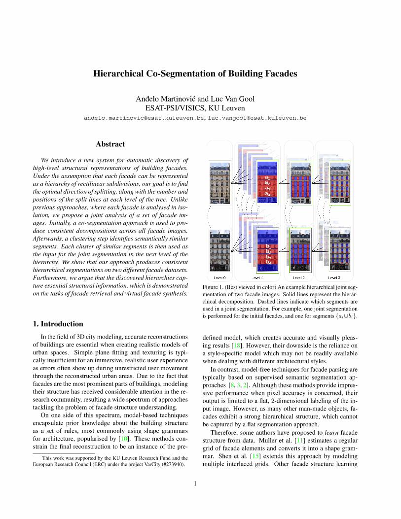
Figure 1. (Best viewed in color) An example hierarchical joint seg-mentation of two facade images. Solid lines represent the hierar-chical decomposition. Dashed lines indicate which segments areused in a joint segmentation. For example, one joint segmentationis performed for the initial facades, and one for segments {𝑎𝑖∪𝑏𝑖}.

defined model, which creates accurate and visually pleas-ing results [18]. However, their downside is the reliance ona style-specific model which may not be readily availablewhen dealing with different architectural styles.

In contrast, model-free techniques for facade parsing aretypically based on supervised semantic segmentation ap-proaches [8, 3, 2]. Although these methods provide impres-sive performance when pixel accuracy is concerned, theiroutput is limited to a flat, 2-dimensional labeling of the in-put image. However, as many other man-made objects, fa-cades exhibit a strong hierarchical structure, which cannotbe captured by a flat segmentation approach.

Therefore, some authors have proposed to learn facadestructure from data. Muller et al. [11] estimates a regulargrid of facade elements and converts it into a shape gram-mar. Shen et al. [15] extends this approach by modelingmultiple interlaced grids. Other facade structure learning

1

methods either depend on user interaction [12, 1, 7] or pre-defined abstractions of the input facades in form of labeledboxes [23] or pixelwise annotations [9, 21].

In this work, we propose to merge the gap between thesupervised facade parsing techniques, which produce im-perfect labelings, and the structured learning approachesthat require clean data to work. Due to the existence of noisein the data, we argue that the structure cannot be reliably es-timated from a single facade image, and thus propose a jointoptimization of a set of facade images. We create consistenthierarchies by performing a joint segmentation of facadesand their parts recursively, see Fig. 1 for an illustration. Thejoint segmentation at each level is performed using a modi-fied linear programming technique originally introduced in[6] for 3D shape segmentation.

The two approaches most similar to ours are the worksof Shen et al. [15] and Van Kaick et al. [19]. In the firstapproach, a hierarchy is created for each facade indepen-dently, resulting in less stable hierarchies with no corre-spondence across images. In the second approach, co-analysis is performed on a set of 3D shapes, but with thekey difference that the hierarchies are first created indepen-dently for each shape and subsequently merged. Further-more, they are limited to an analysis of binary trees, whileour approach allows us to create 𝑛-ary trees from the outset.

2. Our approach

We start with a set of𝑁 facade images F and their noisysemantic segmentations (labelings) L. We obtain the lat-ter by running the first two layers of [8], which provide la-beling results with the highest pixel accuracy, without in-troducing any explicit architectural knowledge. Other ap-proaches for semantic segmentation could also be used,such as [3, 2]. Our main assumption is that the facades fol-low the Manhattan-world assumption, and can be decom-posed by recursive splitting in the vertical and horizontaldirection. This is a common assumption used by a largenumber of previous works in urban modeling [22, 15, 3, 18]which does not preclude the existence of non-rectangularelements (e.g. round windows) since they can still be repre-sented with a bounding box. We define a scope 𝑧 as an axis-aligned bounding box which contains a non-empty area ofan image and its corresponding labeling. The initial set ofimages is thus converted to a set of 𝑁 scopes Z = {𝑧𝑖},each scope completely covering one facade image.

At every step of the hierarchy, we want to find the opti-mal segmentations of all scopes, such that the created seg-ments are consistent across scopes. Due to the Manhattanassumption, we can restrict our search by considering onlysegments generated by splitting the scope in one of the mainsplitting directions. A valid 𝑘-way segmentation of a scopethus consists of 𝑘 adjacent segments separated by 𝑘 − 1splitting lines. A brute-force approach to finding the con-

sistent segmentations would be to consider every possiblecombination of split lines in each scope, and selecting thecombination which maximizes some predefined consistencyscore. Since this would be too computationally expensive,we reduce the dimensionality of the problem by limitingthe number of allowed split line positions. This is done byfirst generating an oversegmentation of each scope into alarge number of smaller segments, or slices, and constrain-ing each segment to be a superset of contiguous slices (seeFig. 2). This idea is similar to using superpixels [13] ingeneral image segmentation, or patches in shape segmenta-tion [6]. The optimal subsets of segments for each scopeare then selected by a modified co-segmentation approachof [6], detailed in Sec. 4. Then, a hierarchical decomposi-tion is created with a recursive approach detailed in Sec. 5.Similar segments across scopes are discovered in a graphclustering step. All segments in one cluster are used as theinput to the joint segmentation stage in the next level of thehierarchy. The process continues until the produced clusterscontain uniform elements (e.g. wall regions) or elementstoo small for subdivision. In Sec. 6 we show that the result-ing hierarchies can be used for structural facade retrievaland sampling of virtual facades. Our contributions are asfollows: (1) A novel approach for creating consistent hier-archical decompositions of building facades. To the best ofour knowledge, we are the first to use a co-segmentation ap-proach in this context; (2) A graph clustering approach forautomatic discovery of semantically similar elements acrossimages; (3) A new tree distance measure for comparing n-ary trees based on sequence matching.

3. Initial segmentation

In order to generate an oversegmentation of a scope, wedefine a support function for placing a split line at each po-sition in the scope:

Υ(𝑧) = Υ𝐼𝐺(F𝑧) ⋅Υ𝐼𝐶(F𝑧) ⋅Υ𝐿𝐵(L𝑧) ⋅Υ𝐿𝐶(L𝑧) (1)

This function aggregates the data support from both theoriginal image and the noisy labeling through the follow-ing four factors, normalized to the interval [0, 1]:Image gradient support Υ𝐼𝐺 [15, 3] promotes placing ofhorizontal (vertical) split lines where horizontal (vertical)edges or gradients are prominent, and vertical (horizontal)edges are rare.Image content support Υ𝐼𝐶 [3] proposes split line posi-tions based on the inverse of the normalized cut betweenthe two created parts of the image.Label border support Υ𝐿𝐵 uses the semantic informationfrom the labeling to penalize lines which split facade ele-ments such as windows, doors and balconies.Label content support Υ𝐿𝐶 : same as Υ𝐼𝐶 , but definedover the labeled image.

Figure 2. A single image-labeling pair (a) is oversegmented into alarge number of slices (b). Randomized segmentations (c) with avarying number of segments create the initial pool of segments.

The next step is to create an oversegmentation of a scopeinto a predefined number of slices. We are looking for atmost 𝐾 split lines (30 in our experiments), correspondingto peaks in the data support function, which split the scopeinto𝐾 + 1 slices.

A peak in a vector is defined as a position where the vec-tor has a higher value than its neighbors, and is preceded bya value lower than a threshold 𝜏 . By setting 𝜏 to a very lowvalue, we initially detect a large number of peaks, most ofthem affected by the noise in the support function. How-ever, we can smooth the support function by convolving itwith a Gaussian window, thus reducing the total amount ofdetected peaks. The peak detection problem is now posedas the search for the best Gaussian window which producesa number of peaks as close as possible to𝐾.

We solve this problem using binary search, setting theinitial lower and upper bound on the Gaussian window sizeto 𝛾𝑙 = 1 and 𝛾𝑢 = ∣Υ(𝑧)∣ respectively. In each step, weconvolve the support function with the Gaussian window ofsize 𝛾𝑚 = (𝛾𝑢+𝛾𝑙)/2. If we detect more peaks than𝐾−1,the search is continued by setting 𝛾𝑙 = 𝛾𝑚. If the numberof peaks is smaller, we set 𝛾𝑢 = 𝛾𝑚. The algorithm finisheswhen 𝛾𝑙 = 𝛾𝑢 or the number of generated peaks is equal to𝐾. The result of this step is a set of 𝐾 + 1 slices C𝑧 , and𝐾 splitting lines l𝑧 , for each scope 𝑧. The support functionevaluated at the splitting line positions Υ(𝑧, 𝑙𝑗) gives us thestrength of each split line, which we use to group the slicesinto segments.

3.1. Segment proposals

Similar to [6], from a set of slices C𝑧 , we generate manyproposal segmentations by varying the number of targetsegments 𝑘 from 1 to 20, and running 250 rounds of ran-domized segmentations for each 𝑘. In each round, we per-form 𝑘-medoid clustering of slices, following the EM pat-tern. We initialize the algorithm by uniformly sampling 𝑘slices as cluster centers. In the M-step, every slice 𝑐𝑖 ∈ Cz

is assigned to the closest cluster center 𝑐𝑚, based on the dis-tance between two slices 𝛿(𝑐1, 𝑐2). We define this distanceas the maximum of all split line strengths Υ between twoslices, which penalizes the creation of segments which spanstrong split lines. If there is another cluster center 𝑐′𝑚 be-tween 𝑐 and 𝑐𝑚, the distance 𝛿(𝑐, 𝑐𝑚) is set to infinity. This

forces the segmentation to contain only contiguous clustersof slices. In the E-step, the medoids are estimated from thecluster members, by minimizing the sum of distances be-tween elements in one cluster.

Typically, many segments generated in this fashion willappear in more than one randomized segmentation. Seg-ments that are generated the most often are the ones mostuseful to us, being less sensitive to randomization and theselected number of target segments. Therefore, we weighteach unique segment 𝑠 by the number of times it appearsover all randomized segmentations of a single scope, i.e.the frequency of appearance is used as the fitness score 𝑤𝑠

of the segment. This simple weighting scheme proved tobe sufficient for the task, as we did not observe any im-provement by using the more elaborate weighting schemefrom [6]. Finally, to reduce the total amount of segmentsfor the subsequent optimization procedure, for each scopewe retain 𝑛 = 100 segments with the highest weight as theset of proposals 𝐼𝑧 , making sure that it contains at least onecomplete segmentation of the scope.

We represent each segment 𝑠 with a vector h(𝑠) which isa concatenation of two types of features:Label features h𝑙(𝑠). Histogram of labels from the entiresegment and from each of its 2𝑥2 subdivisions. The result-ing feature vector captures the coarse distribution of labels.Image features h𝑖(𝑠). Histogram of visual words. DenseSIFT features are extracted from all images, followed byK-means clustering into a codebook of 256 visual words.

Finally, to measure the dissimilarity between two seg-ments, we introduce a distance measure based on the his-togram intersection between the feature vectors:

𝑑(𝑠, 𝑠′) = 1−∑

𝑖𝑚𝑖𝑛(h𝑖(𝑠),h𝑖(𝑠′))∑

𝑖 h𝑖(𝑠′)(2)

4. Co-segmentation

The purpose of the co-segmentation step is to find thebest subset of segments for each scope, such that they aresalient in each scope and consistent across scopes. We fol-low the same basic algorithm which was introduced for jointsegmentation of 3D shapes [6]. In this section, we summa-rize the basic algorithm, with emphasis on the main differ-ences introduced in our work.

4.1. Pairwise co-segmentation

Given two scopes 𝑧1 and 𝑧2 and their correspondingsets of proposal segments 𝐼1 and 𝐼2, the pairwise co-segmentation searches for the best valid subsets of segments𝑆1 ⊆ 𝐼1 and 𝑆2 ⊆ 𝐼2, by maximizing both the quality of in-dividual segmentations, and the consistency between them.A subset of segments is considered valid only if the selectedsegments cover the entire scope without overlapping. Theconsistency between two scopes is modeled through two

many-to-one mappings 𝑀𝑖𝑗 ⊂ 𝑆𝑖 × 𝑆𝑗 , from segments in𝑆1 to segments in 𝑆2, and vice versa. The many-to-onemappings allow us to match scopes with different amountof corresponding parts. Thus, each segment in one scopewill be mapped to at most one segment in the other scope.The maximization can be written as

max𝑆1,𝑆2,𝑀12,𝑀21

∑𝑠∈𝑆1∪𝑆2

𝑟𝑠𝑤𝑠 + 𝜆∑

(𝑠,𝑠′)∈{𝑀12,𝑀21}𝑟𝑠𝑤(𝑠,𝑠′) (3)

where the parameter 𝜆 (0.1 in our experiments) weighs therelative importance of the segmentation (left) and consis-tency scores (right). The segmentation score is a normal-ized sum of segment weights 𝑤𝑠, defined in Sec. 3.1. Thenormalization factor is the relative size of the segment 𝑠 inthe scope 𝑧: 𝑟𝑠 = area(𝑠)/area(𝑧).

The consistency term is a normalized sum of similarityweights between all segment pairs (𝑠, 𝑠′) induced by eachof the two mappings. The similarity is determined based onthe distance measure 𝑑 between two segments (Sec. 3.1):

𝑤(𝑠,𝑠′) = 𝑒𝑥𝑝

(−𝑑

2(𝑠, 𝑠′)2𝜎2

)(4)

In our experiments, 𝜎 is set to half the maximum distancebetween all pairs of most similar segments.

4.1.1 Integer programming formulation

The maximization problem from Eq. 3 can be reformulatedas an integer program [6]. For for every segment 𝑠 ∈ 𝐼𝑖,an indicator variable 𝑥𝑠 is introduced, and defined to be𝑥𝑠 = 1 when the segment is selected, and 0 otherwise. Ad-ditionally, for every pair of segments (𝑠, 𝑠′) ∈ 𝐼𝑖 × 𝐼𝑗 , theindicator variable 𝑦(𝑠,𝑠′) is defined to be 1 when this pair isselected in the mapping 𝑀𝑖𝑗 . The objective function fromEq. 3 is then reformulated as follows:

max∑

𝑖∈{1,2}x𝑇𝑖 w

𝑠𝑒𝑔𝑖 + 𝜆

∑𝑖𝑗∈{12,21}

y𝑇𝑖𝑗w

𝑐𝑜𝑟𝑖𝑗 (5)

where x𝑖 and w𝑠𝑒𝑔𝑖 represent all segment indicators in 𝐼𝑖

and their normalized weights. Likewise, y𝑖𝑗 is a binaryvector of all pair indicators in 𝐼𝑖 × 𝐼𝑗 , and w𝑐𝑜𝑟

𝑖𝑗 are theirnormalized similarity weights. The first set of constraints inthe integer program states that the selected segments mustcover the entire scope 𝑧𝑖, without overlapping:∑

𝑠∈𝑐𝑜𝑣𝑒𝑟(𝑐)

𝑥𝑠 = 1 ∀𝑐 ∈ C𝑧𝑖 (6)

where 𝑐𝑜𝑣𝑒𝑟(𝑐) is the set of all segments that contain slice𝑐. Secondly, each segment of 𝐼𝑖 can map to at most onesegment in 𝐼𝑗 , which itself has to be selected:∑

𝑠′∈𝐼𝑗

𝑦(𝑠,𝑠′) ≤ 𝑥𝑠 ∀𝑠 ∈ 𝐼𝑖 (7)

𝑦(𝑠,𝑠′) ≤ 𝑥𝑠′ ∀(𝑠, 𝑠′) ∈ 𝐼𝑖 × 𝐼𝑗 (8)

The integer problem (IP) is obtained by adding the inte-grality constraints on the 𝑥 and 𝑦 variables. Note that ourprogram contains 2𝑛 + 4𝑛2 integer variables, unlike [6],where adjacency constraints create 2𝑛4 additional variables.In our experiments, using the adjacency term did not re-sult in any noticeable improvement. Another difference isthat we solve the IP by relaxing the integrality constraintsonly on the 𝑦 variables, resulting in a mixed-integer lin-ear program (MILP) with 2𝑛 integrality constraints. Thisapproach gives us a tighter bound on the IP solution thanwe would obtain by relaxing all variables. Although theworst-case complexity of this MILP is 𝑂(22𝑛), in practicethe constraints (7) and (8) allow for a quick convergence ofbranch-and-cut methods, such as the MOSEK MILP solverin the CVX software package [5]. For 𝑛 = 100, the opti-mal solution is usually reached within a few seconds on an8-core machine. The fractional 𝑦 variables are subsequentlyrounded to the closest integer, respecting the constraints.

Segment filtering. After the optimization in Eq. 5 hasbeen performed for every pair of scopes, we introduce anadditional filtering step. For each scope, we keep only thesegments that are selected in at least one of the pairwiseoptimizations. By discarding the remaining segments, wereduce the computational burden in the subsequent stages.

4.2. Multiway co-segmentation

A joint segmentation of all scopes is performed by a gen-eralization of Eq. 5 to 𝑁 scopes:

max𝑁∑𝑖=1

x𝑇𝑖 w

𝑠𝑒𝑔𝑖 +

𝜆

𝑁 − 1

𝑁∑𝑖=1

𝑁∑𝑗=1

𝑖∕=𝑗

y𝑇𝑖𝑗w

𝑐𝑜𝑟𝑖𝑗 (9)

Note that the segment filtering step reduces the size of wvectors compared to Eq. 5. The resulting optimization isagain solved with CVX, but due to its higher complexity,we constrain the maximum run-time of the solver to 30 min-utes. In our experience, this was enough to reach a solutionwith a sufficiently small optimality gap. An approximateblock-coordinate procedure as in [6] could be employed toincrease the speed of optimization, but with no optimalityguarantees.

5. Hierarchical co-segmentation

The co-segmentation step results in a flat segmentationof each scope, with mappings between corresponding seg-ments in different scopes. The next step is to create a hi-erarchical decomposition of each facade. The first step to-wards this goal is finding subsets of semantically identicalelements, which can be segmented jointly in the next stepof the hierarchy.

Figure 3. (Best viewed in color) Hierarchical joint segmentation of facade images: (a) ECP dataset. (b) Gruenderzeit dataset. Each clusterof similar elements in one level of the hierarchy is represented with the same overlay color, which corresponds to the border color in thenext level. Due to space restrictions, only a subset of the hierarchy is shown.

5.1. Segment clustering

We represent the segments selected in all scopes by thejoint segmentation into one directed, weighted assignmentgraph 𝐺 = (𝑉,𝐸). Each node in the set 𝑉 corresponds toa selected segment 𝑠𝑖, i.e. a segment for which 𝑥𝑖 = 1. 𝐸is a set of directed edges, where node 𝑣𝑖 is connected to 𝑣𝑗if the value of the corresponding 𝑦𝑖𝑗 variable is equal to 1.The weight of each edge 𝑒𝑖𝑗 is defined in Eq. 4.

Our key observation is that the groups of similar ele-ments will form dense clusters in the graph 𝐺. By discov-ering these clusters, we will also find self-similarities in theinput scopes, a feature not modeled by the joint segmen-tation itself. Thus, our goal is to determine the groups ofsegments which correspond to each other, within and acrossscopes. To this end, we run spectral clustering [20] on thegraph 𝐺. We calculate the normalized graph Laplacian asin [16], and use its eigenvalue decomposition to find thenumber of clusters 𝜅. Based on the eigengap heuristic, wesort the eigenvalues 𝜆𝑖 in ascending order, and pick 𝜅 as𝑎𝑟𝑔𝑚𝑎𝑥𝑖(𝜆𝑖+1 − 𝜆𝑖).

There is a possibility that after the clustering step, twoneighboring segments in a scope are assigned to the samecluster, e.g. two wall parts next to each other. In thesecases, we simplify the final segmentation by merging thosesegments into one. However, this must not be done indis-criminately, since there are cases when we expect neighbor-ing segments of the same class (e.g. two floors). We mergetwo neighboring segments only if their potential merger hasa small distance 𝑑 to the remaining segments in the cluster.

5.2. Hierarchy creation

Initially,𝑁 segmentation trees are created, each contain-ing a single root node, corresponding to the whole facade.After performing the co-segmentation and clustering, everytree is augmented with 𝜅 children nodes, one for each clus-ter. In Fig. 3 the trees are merged and the same-cluster seg-ments overlaid with the same color. These segments nowbecome new sets of scopes for the next level of joint seg-mentation, performed recursively on each cluster. The re-cursion stops when either the average scope size in the di-rection of splitting is smaller than a predefined size, or thescopes in the set are uniform in appearance.

The direction of splitting for each node in the hierarchy isdetermined adaptively. We perform the joint segmentationin both directions, and select the one which gives a moreconsistent joint segmentation, based on the similarity be-tween a pair of scopes 𝑧𝑖 and 𝑧𝑗 [6]:

𝑤(𝑧𝑖, 𝑧𝑗) = y𝑇𝑖𝑗w

𝑐𝑜𝑟𝑖𝑗 + y𝑇

𝑗𝑖w𝑐𝑜𝑟𝑗𝑖 , 𝑤 ∈ [0, 2] (10)

5.3. Segment synchronization

As we go deeper in the hierarchy, the number of scopesto be jointly segmented increases dramatically (e.g. 20 fa-cades result in ~80 floors and ~400 windows). We can re-duce the computational burden for the joint segmentationsteps further down in the hierarchy by making the followingobservation: within one cluster, two scopes with a commonparent node are more alike than scopes originating from dif-ferent parents. Therefore, instead of considering each of

these scopes separately, we perform segment synchroniza-tion. First, for each set Ψ of same-cluster scopes originatingfrom the same node, we average their data support func-tions:

Υ𝑎𝑣𝑔 =1

∣Ψ∣∑𝑠∈Ψ

Υ(𝑠) (11)

and create a representative scope by averaging the featurevectors of all scopes in Ψ. This scope replaces all scopesin Ψ during the joint segmentation. Afterwards, the dis-covered segment borders are back-projected to the originalscopes.

Fig. 1 illustrates the process of synchronization: floors 𝑎𝑖are synchronized: they originate from the same facade, sothey are segmented in the same way. However, their hierar-chies are allowed to differ. As can be seen in the next levelof the hierarchy, window tiles in floors 𝑎𝑖 are synchronized,but different from the synchronized tiles of floors 𝑏𝑖. Thisallows us to model local differences, while still correctlycapturing the global correspondence.

6. Results

In this section we show some qualitative results of thejoint hierarchical segmentation, and evaluate the approachon the task of facade retrieval. Finally, we show how virtualfacade layouts can be generated from the induced hierarchy.

6.1. Experimental setup

The main evaluation of our approach is performed onthe well-established ECP facades dataset [18], containing104 images of buildings in Paris. Since all facades in thisdataset follow the same Haussmannian architectural style,it is an ideal candidate for our joint segmentation approach.We deal with 7 semantic labels in this dataset, namely{𝑤𝑖𝑛𝑑𝑜𝑤,𝑤𝑎𝑙𝑙, 𝑏𝑎𝑙𝑐𝑜𝑛𝑦, 𝑑𝑜𝑜𝑟, 𝑟𝑜𝑜𝑓, 𝑠𝑘𝑦, 𝑠ℎ𝑜𝑝}. We alsotest our approach on a subset of [14], consisting of 30 im-ages in Gruenderzeit style, annotated with a smaller set oflabels: {𝑤𝑖𝑛𝑑𝑜𝑤,𝑤𝑎𝑙𝑙, 𝑑𝑜𝑜𝑟}. Since we use the output ofa supervised facade parsing approach [8] as the input to ourapproach, we are limited to the analysis of the test set. Tocover the entire ECP dataset, we repeat our experiments 5times, in each fold using different 20 images as the test set,and average the results.

6.2. Hierarchical co-segmentation

In Fig. 3 we visualize the results of our approach on asubset of ECP and Gruenderzeit dataset, respectively. Dueto space limitations, here we show only some nodes in thehierarchy, while the full results can be found in the supple-mentary material.

The first row of Fig. 3 (a) shows the consistent first-levelsegmentation of the Parisian facades. The coloring corre-sponds to the different clusters discovered in the data. Our

system has automatically detected 6 clusters of similar ele-ments, roughly corresponding to the regions of sky, roof andshop, ledges (red) and two types of floors: regular (green)and floor with running balcony (purple). The consistent seg-mentation reveals that running balconies usually appear inthe second and fifth floor, which is one of the distinguishingproperties of Haussmannian architecture. We can also seethat the floors with running balconies are split differentlythan the regular floors in the next level of the hierarchy.

In the Gruenderzeit dataset, we can solely separate floorsfrom the wall regions, since there are only three semantic la-bels in the annotations. Even in this case, the hierarchicalsegmentation produces reasonable results, splitting floorsinto window tiles, which are further subdivided into win-dow and wall regions.

6.3. Facade retrieval

In facade retrieval, a query facade is presented to the sys-tem. The query is then compared to a set of known facadesbased on a pre-defined distance measure. These facades arethen re-ranked based on their distance to the query facade,and top𝐾 ranked facades are returned as output.

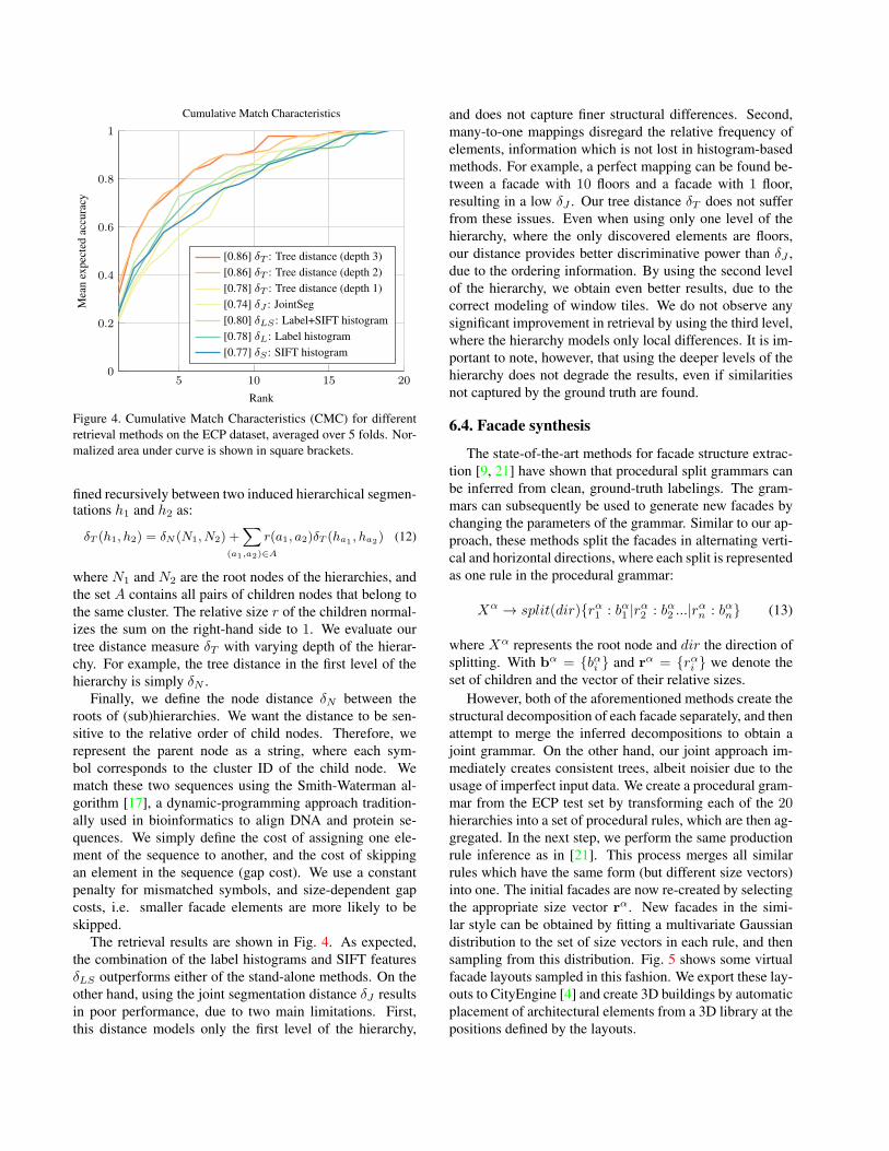
In this section, we demonstrate that our hierarchical rep-resentation of facade structures can be used for retrieval ofstructurally similar facades, rather than those similar in lo-cal appearance. We follow the protocol for facade compar-ison introduced in [21] for the ECP dataset. The gold stan-dard distance 𝛿𝐺𝑇 between two facades is defined as the to-tal number of architectural changes: number of floors, num-ber of window columns, position of the running balconiesand doors. For each facade in the set, all other facadesare re-ranked in the ascending order of 𝛿𝐺𝑇 , and the onewith the smallest distance is kept as the ground-truth near-est neighbor. Once the ground truth ranking is established,various retrieval methods are evaluated using the Cumula-tive Match Characteristic (CMC). This measure counts thepercentage of correctly retrieved results (gold distance near-est neighbors) in the top-𝐾 ranking. When 𝐾 is equal tothe dataset size, all facades are retrieved, resulting in CMCvalue of 1 for any method.

We test the retrieval results with several different meth-ods, and show the results in Fig. 4. As the first baselinefor facade comparison, we create the histograms of seman-tic labels in each image, and use the histogram intersec-tion measure as the distance 𝛿𝐿. Second, we use the his-tograms of dense SIFT features coded into a vocabulary of256 visual words, to obtain the distance 𝛿𝑆 . A combineddistance 𝛿𝐿𝑆 is calculated by concatenating the two afore-mentioned histograms. Additionally, we evaluate the dis-tance 𝛿𝐽 = 2 − 𝑤(𝑧𝑖, 𝑧𝑗), measuring the dissimilarity ofscopes in the first-level joint segmentation step (Eq. 10).

In order to test our hierarchical method, we introducea new measure for tree distance 𝛿𝑇 . The distance is de-

5 10 15 200

0.2

0.4

0.6

0.8

1

Rank

Mea

nex

pect

edac

cura

cy

Cumulative Match Characteristics

[0.86] 𝛿𝑇 : Tree distance (depth 3)[0.86] 𝛿𝑇 : Tree distance (depth 2)[0.78] 𝛿𝑇 : Tree distance (depth 1)[0.74] 𝛿𝐽 : JointSeg[0.80] 𝛿𝐿𝑆 : Label+SIFT histogram[0.78] 𝛿𝐿: Label histogram[0.77] 𝛿𝑆 : SIFT histogram

Figure 4. Cumulative Match Characteristics (CMC) for differentretrieval methods on the ECP dataset, averaged over 5 folds. Nor-malized area under curve is shown in square brackets.

fined recursively between two induced hierarchical segmen-tations ℎ1 and ℎ2 as:

𝛿𝑇 (ℎ1, ℎ2) = 𝛿𝑁 (𝑁1, 𝑁2) +∑

(𝑎1,𝑎2)∈𝐴

𝑟(𝑎1, 𝑎2)𝛿𝑇 (ℎ𝑎1 , ℎ𝑎2) (12)

where 𝑁1 and 𝑁2 are the root nodes of the hierarchies, andthe set 𝐴 contains all pairs of children nodes that belong tothe same cluster. The relative size 𝑟 of the children normal-izes the sum on the right-hand side to 1. We evaluate ourtree distance measure 𝛿𝑇 with varying depth of the hierar-chy. For example, the tree distance in the first level of thehierarchy is simply 𝛿𝑁 .

Finally, we define the node distance 𝛿𝑁 between theroots of (sub)hierarchies. We want the distance to be sen-sitive to the relative order of child nodes. Therefore, werepresent the parent node as a string, where each sym-bol corresponds to the cluster ID of the child node. Wematch these two sequences using the Smith-Waterman al-gorithm [17], a dynamic-programming approach tradition-ally used in bioinformatics to align DNA and protein se-quences. We simply define the cost of assigning one ele-ment of the sequence to another, and the cost of skippingan element in the sequence (gap cost). We use a constantpenalty for mismatched symbols, and size-dependent gapcosts, i.e. smaller facade elements are more likely to beskipped.

The retrieval results are shown in Fig. 4. As expected,the combination of the label histograms and SIFT features𝛿𝐿𝑆 outperforms either of the stand-alone methods. On theother hand, using the joint segmentation distance 𝛿𝐽 resultsin poor performance, due to two main limitations. First,this distance models only the first level of the hierarchy,

and does not capture finer structural differences. Second,many-to-one mappings disregard the relative frequency ofelements, information which is not lost in histogram-basedmethods. For example, a perfect mapping can be found be-tween a facade with 10 floors and a facade with 1 floor,resulting in a low 𝛿𝐽 . Our tree distance 𝛿𝑇 does not sufferfrom these issues. Even when using only one level of thehierarchy, where the only discovered elements are floors,our distance provides better discriminative power than 𝛿𝐽 ,due to the ordering information. By using the second levelof the hierarchy, we obtain even better results, due to thecorrect modeling of window tiles. We do not observe anysignificant improvement in retrieval by using the third level,where the hierarchy models only local differences. It is im-portant to note, however, that using the deeper levels of thehierarchy does not degrade the results, even if similaritiesnot captured by the ground truth are found.

6.4. Facade synthesis

The state-of-the-art methods for facade structure extrac-tion [9, 21] have shown that procedural split grammars canbe inferred from clean, ground-truth labelings. The gram-mars can subsequently be used to generate new facades bychanging the parameters of the grammar. Similar to our ap-proach, these methods split the facades in alternating verti-cal and horizontal directions, where each split is representedas one rule in the procedural grammar:

𝑋𝛼 → 𝑠𝑝𝑙𝑖𝑡(𝑑𝑖𝑟){𝑟𝛼1 : 𝑏𝛼1 ∣𝑟𝛼2 : 𝑏𝛼2 ...∣𝑟𝛼𝑛 : 𝑏𝛼𝑛} (13)

where 𝑋𝛼 represents the root node and 𝑑𝑖𝑟 the direction ofsplitting. With b𝛼 = {𝑏𝛼𝑖 } and r𝛼 = {𝑟𝛼𝑖 } we denote theset of children and the vector of their relative sizes.

However, both of the aforementioned methods create thestructural decomposition of each facade separately, and thenattempt to merge the inferred decompositions to obtain ajoint grammar. On the other hand, our joint approach im-mediately creates consistent trees, albeit noisier due to theusage of imperfect input data. We create a procedural gram-mar from the ECP test set by transforming each of the 20hierarchies into a set of procedural rules, which are then ag-gregated. In the next step, we perform the same productionrule inference as in [21]. This process merges all similarrules which have the same form (but different size vectors)into one. The initial facades are now re-created by selectingthe appropriate size vector r𝛼. New facades in the simi-lar style can be obtained by fitting a multivariate Gaussiandistribution to the set of size vectors in each rule, and thensampling from this distribution. Fig. 5 shows some virtualfacade layouts sampled in this fashion. We export these lay-outs to CityEngine [4] and create 3D buildings by automaticplacement of architectural elements from a 3D library at thepositions defined by the layouts.

Figure 5. Synthesis of virtual facade layouts. The sampled layoutsare represented as procedural split grammars and converted into3D models with CityEngine.

7. Conclusion

We have introduced a system for higher-level under-standing of building facades through a joint hierarchical de-composition approach. Unlike most previous facade struc-ture learning approaches, which rely on user interaction orground truth annotations, we show that facade structure canbe induced even by using noisy inputs. Our key observationis that consistent hierarchies can be created by performinga joint segmentation approach on each level of the hierar-chy. The joint segmentation allows us to produce stable,consistent segmentations across images, despite the noisepresent in the input data. Moreover, the induced hierarchiesare a meaningful semantic representation of the building fa-cade, which we demonstrate on the task of structural fa-cade retrieval. We also convert the hierarchies into proce-dural grammars and use them to sample new facade designs,which respect the layout of the original facades.

In future work, we plan to further reduce the dependencyon image labelings, and induce structure solely from im-ages. Furthermore, feedback can be added in the hierarchyconstruction, to reduce the effect of error propagation to thelower levels of the hierarchy. Finally, we will investigatehow to model different kinds of structural decompositions,such as repetition and symmetry.

References

[1] F. Bao, M. Schwarz, and P. Wonka. Procedural facade varia-tions from a single layout. ACM Trans.Graph., 32(1), 2013.2

[2] A. Cohen, A. G. Schwing, and M. Pollefeys. Efficient struc-tured parsing of facades using dynamic programming. InCVPR, 2014. 1, 2

[3] D. Dai, M. Prasad, G. Schmitt, and L. Van Gool. Learningdomain knowledge for facade labeling. In ECCV, 2012. 1, 2

[4] Esri. CityEngine. http://www.esri.com/software/cityengine,2013. 7

[5] M. Grant and S. Boyd. CVX: Matlab software for disciplinedconvex programming. http://cvxr.com/cvx, Mar. 2014. 4

[6] Q. Huang, V. Koltun, and L. Guibas. Joint shape seg-mentation with linear programming. ACM Trans. Graph.,30(6):125:1–125:12, 2011. 2, 3, 4, 5

[7] J. Lin, D. Cohen-Or, H. R. Zhang, C. Liang, A. Sharf,O. Deussen, and B. Chen. Structure-preserving retargetingof irregular 3d architecture. ACM Trans.Graph., 30(6), 2011.2

[8] A. Martinovic, M. Mathias, J. Weissenberg, and L. Van Gool.A three-layered approach to facade parsing. In ECCV, 2012.1, 2, 6

[9] A. Martinovic and L. Van Gool. Bayesian grammar learningfor inverse procedural modeling. In CVPR, 2013. 2, 7

[10] P. Müller, P. Wonka, S. Haegler, A. Ulmer, and L. Van Gool.Procedural modeling of buildings. In SIGGRAPH, 2006. 1

[11] P. Müller, G. Zeng, P. Wonka, and L. J. V. Gool. Image-based procedural modeling of facades. ACM Trans. Graph.,26(3):85, 2007. 1

[12] P. Musialski, M. Wimmer, and P. Wonka. Interactivecoherence-based facade modeling. Computer Graphics Fo-rum, 31(2pt3):661–670, 2012. 2

[13] X. Ren and J. Malik. Learning a classification model forsegmentation. In ICCV, volume 1, pages 10–17, 2003. 2

[14] H. Riemenschneider, U. Krispel, W. Thaller, M. Donoser,S. Havemann, D. W. Fellner, and H. Bischof. Irregular lat-tices for complex shape grammar facade parsing. In CVPR,2012. 6

[15] C.-H. Shen, S.-S. Huang, H. Fu, and S.-M. Hu. Adaptivepartitioning of urban facades. ACM Trans.Graph., 30(6):184,2011. 1, 2

[16] J. Shi and J. Malik. Normalized cuts and image segmenta-tion. IEEE TPAMI, 22(8):888–905, Aug 2000. 5

[17] T. Smith and M. Waterman. Identification of commonmolecular subsequences. Journal of Molecular Biology,147(1):195–197, 1981. 7

[18] O. Teboul, I. Kokkinos, L. Simon, P. Koutsourakis, andN. Paragios. Parsing facades with shape grammars and rein-forcement learning. IEEE TPAMI, 35(7):1744–1756, 2013.1, 2, 6

[19] O. van Kaick, K. Xu, H. Zhang, Y. Wang, S. Sun, A. Shamir,and D. Cohen-Or. Co-hierarchical analysis of shape struc-tures. ACM Trans.Graph., 32(4), 2013. 2

[20] U. von Luxburg. A tutorial on spectral clustering. CoRR,abs/0711.0189, 2007. 5

[21] J. Weissenberg, H. Riemenschneider, M. Prasad, and L. VanGool. Is there a procdural logic to architecture? In CVPR,2013. 2, 6, 7

[22] P. Wonka, M. Wimmer, F. X. Sillion, and W. Ribarsky. In-stant architecture. SIGGRAPH, 22(3):669–677, 2003. 2

[23] H. Zhang, K. Xu, W. Jiang, J. Lin, D. Cohen-Or, andB. Chen. Layered analysis of irregular facades via symmetrymaximization. ACM Trans.Graph., 32(4):121:1–13, 2013. 2