1 IntroductionThis paper considers elliptic partial differential equations (PDEs) of the form
�r � .a.x/ru.x//C b.x/u.x/ D f .x/; x 2 � � Rd ;(1.1)
with appropriate boundary conditions on @�, where a.x/, b.x/, and f .x/ are givenfunctions, and d D 2 or 3. Such equations are of fundamental importance inscience and engineering and encompass (perhaps with minor modification) manyof the PDEs of classical physics, including the Laplace, Helmholtz, Stokes, andtime-harmonic Maxwell equations. We will further assume that (1.1) is not highlyindefinite. Discretization using local schemes such as finite differences or finiteelements then leads to a linear system
Au D f;(1.2)
where A 2 RN�N is sparse with u and f the discrete analogues of u.x/ and f .x/,respectively. This paper is concerned with the efficient factorization and solutionof such systems.
1.1 Previous WorkA large part of modern numerical analysis and scientific computing has been de-
voted to the solution of (1.2). We classify existing approaches into several groups.The first consists of classical direct methods like Gaussian elimination or otherstandard matrix factorizations [19], which compute the solution exactly (in princi-ple, to machine precision, up to conditioning) without iteration. Naive implemen-tations generally have O.N 3/ complexity but can be heavily accelerated by ex-ploiting sparsity [10]. A key example is the nested dissection multifrontal method(MF) [12, 15, 33], which performs elimination according to a special hierarchy ofseparator fronts in order to minimize fill-in. These fronts correspond geometricallyto the cell interfaces in a domain partitioning and grow as O.N 1=2/ in two dimen-sions (2D) andO.N 2=3/ in three dimensions (3D), resulting in solver complexitiesof O.N 3=2/ and O.N 2/, respectively. This is a significant improvement and, in-deed, MF has proven very effective in many environments. However, it remainsunsuitable for truly large-scale problems, especially in 3D.
The second group is that of iterative methods [36], with conjugate gradient(CG) [29, 41] and multigrid [7, 24, 47] among the most popular techniques. Thesetypically work well when a.x/ and b.x/ are smooth, in which case the number ofiterations required is small and optimal O.N/ complexity can be achieved. How-ever, the iteration count can grow rapidly in the presence of ill-conditioning, whichcan arise when the coefficient functions lack regularity or have high contrast. Insuch cases, convergence can be delicate and specialized preconditioners are oftenrequired. Furthermore, iterative methods can be inefficient for systems involvingmultiple right-hand sides or low-rank updates, which is an important setting formany applications of increasing interest, including time stepping, inverse prob-lems, and design.
The third group covers rank-structured direct solvers, which exploit the obser-vation that certain off-diagonal blocks of A and A�1 are numerically low-rank[4–6, 8] in order to dramatically lower the cost. The seminal work in this area isdue to Hackbusch et al. [25–27], whose H - and H 2-matrices have been shownto achieve linear or quasilinear complexity. These methods were originally intro-duced for integral equations characterized by structured dense matrices but applyalso to PDEs as a special case. Although their work has had significant theoreticalimpact, in practice the constants implicit in the asymptotic scalings tend to be quitelarge due to the recursive nature of the inversion algorithms, the use of expensivehierarchical matrix-matrix multiplication, and the lack of sparsity optimizations.
More recent developments aimed at improving practical performance have com-bined MF with structured matrix algebra on the dense frontal matrices only. Thisbetter exploits the inherent sparsity of A and has been carried out under both theH - [20, 39, 40] and hierarchically semiseparable (HSS) [16, 17, 42–44] matrixframeworks, among other related schemes [1,2,34]. Those under the former retain
FIGURE 1.1. Schematic of MF (top) and HIF-DE (bottom) in 2D. Thegray box (left) represents a uniformly discretized square; the lines in theinterior of the boxes (right) denote the remaining DOFs after each levelof elimination or skeletonization.
their quasilinear complexities and have improved constants but can still be some-what expensive. On the other hand, those using HSS operations, which usuallyhave much more favorable constants, are optimal in 2D but require O.N 4=3/ workin 3D. In principle, it is possible to further reduce this toO.N/ work by using mul-tilayer HSS representations, but this procedure is quite complicated and has yet tobe achieved.
1.2 ContributionsIn this paper, we introduce the hierarchical interpolative factorization for PDEs
(HIF-DE), which produces an approximate generalized LU/LDL decompositionof A with linear or quasilinear complexity estimates. HIF-DE is based on MF butaugments it with frontal compression using a matrix sparsification technique thatwe call skeletonization. The resulting algorithm is similar in structure to the accel-erated MF solvers above and is sufficient for estimated scalings ofO.N/ in 2D andO.N logN/ in 3D. Unlike [16, 17, 20, 39, 40, 44], however, which keep the entirefronts but work with them implicitly using fast structured methods, our sparsifi-cation approach allows us to reduce the fronts explicitly (see also [42, 43]). Thisobviates the need for internal hierarchical matrix representations and substantiallysimplifies the algorithm. Importantly, it also makes any additional compressionstraightforward to accommodate, thereby providing a ready means to achieve esti-matedO.N/ complexity in 3D by skeletonizing the compressed fronts themselves.This corresponds geometrically to a recursive dimensional reduction, whose inter-pretation is directly enabled by the skeletonization formalism.
Figure 1.1 shows a schematic of HIF-DE as compared to MF in 2D. In MF(top), the domain is partitioned by a set of separators into “interior” square cells ateach level of a tree hierarchy. Each cell is eliminated starting from the finest level
4 K. L. HO AND L. YING
to the coarsest, leaving degrees of freedom (DOFs) only on the separators, whichconstitute the so-called fronts. This process can be understood as the compressionof data from the cells to their interfaces, which evidently grow as we march up thetree, ultimately leading to the observed O.N 3=2/ complexity.
In contrast, in HIF-DE (bottom), we start by eliminating interior cells as inMF but, before proceeding further, perform an additional level of compressionby skeletonizing the separators. For this, we view the separator DOFs as livingon the interfacial edges of the interior cells then skeletonize each cell edge. Thisrespects the one-dimensional (1D) structure of the separator geometry and allowsmore DOFs to be eliminated, in effect reducing each edge to only those DOFsnear its boundary. Significantly, this occurs without any loss of existing sparsity.The combination of interior cell elimination and edge skeletonization is then re-peated up the tree, with the result that the frontal growth is now suppressed. Thereduction from 2D (square cells) to 1D (edges) to zero dimensions (0D) (points)is completely explicit. Extension to 3D is immediate by eliminating interior cubiccells and then skeletonizing cubic faces at each level to execute a reduction from3D to 2D to 1D at a total estimated cost ofO.N logN/. We can further reduce thisto O.N/ (but at the price of introducing some fill-in) by adding subsequent cubicedge skeletonization at each level for full reduction to 0D. This tight control of thefront size is critical for achieving near-optimal scaling.
Once the factorization has been constructed, it can be used to rapidly applyA�1 and therefore serves as a fast direct solver or preconditioner, depending onthe accuracy. (It can also be used to apply A itself, but this is not particularlyadvantageous since A typically has only O.N/ nonzeros.) Other capabilities arepossible, too, though they will not be pursued here.
HIF-DE can also be understood in relation to the somewhat more general hi-erarchical interpolative factorization for integral equations (HIF-IE) described inthe companion paper [31], which, like other structured dense methods, can applyto PDEs as a special case. However, HIF-IE does not make use of sparsity and so isnot very competitive in practice. HIF-DE remedies this by essentially embeddingHIF-IE into the framework of MF in order to maximally exploit sparsity.
Extensive numerical experiments reveal strong evidence for quasilinear com-plexity and demonstrate that HIF-DE can accurately approximate elliptic partialdifferential operators in a variety of settings with high practical efficiency.
1.3 OutlineThe remainder of this paper is organized as follows. In Section 2, we introduce
the basic tools needed for our algorithm, including our new skeletonization opera-tion. In Section 3, we review MF, which will serve to establish the necessary algo-rithmic foundation as well as to highlight its fundamental difficulties. In Section4, we present HIF-DE as an extension of MF with frontal skeletonization corre-sponding to recursive dimensional reduction. Although we cannot yet provide arigorous complexity analysis, estimates based on well-supported rank assumptions
suggest that HIF-DE achieves linear or quasilinear complexity. This conjecture isborne out by numerical experiments, which we detail in Section 5. Finally, Section6 concludes with some discussion and future directions.
2 PreliminariesIn this section, we first list our notational conventions and then describe the basic
elements of our algorithm.Uppercase letters will generally denote matrices, while the lowercase letters c,
p, q, r , and s denote ordered sets of indices, each of which is associated with aDOF in the problem. For a given index set c, its cardinality is written jcj. The(unordered) complement of c is given by cc, with the parent set to be understoodfrom the context. The uppercase letter C is reserved to denote a collection ofdisjoint index sets.
Given a matrix A, Apq is the submatrix with rows and columns restricted tothe index sets p and q, respectively. We also use the MATLAB® notation AW;q todenote the submatrix with columns restricted to q. The neighbor set of an indexset c with respect to A is then cN D fi … c W Ai;c or Ac;i ¤ 0g.
Throughout, k � k refers to the 2-norm.For simplicity, we hereafter assume that the matrix A in (1.2) is symmetric,
though this is not strictly necessary [31].
2.1 Sparse EliminationLet
A D
24App ATqp
Aqp Aqq ATrq
Arq Arr
35(2.1)
be a symmetric matrix defined over the indices .p; q; r/. This matrix structure oftenappears in sparse PDE problems such as (1.2), where, for example, p correspondsto the interior DOFs of a region D , q to the DOFs on the boundary @D , and r tothe external region � n xD , which should be thought of as large. In this setting, theDOFs p and r are separated by q and hence do not directly interact, resulting inthe form (2.1).
Our first tool is quite standard and concerns the efficient elimination of DOFsfrom such sparse matrices.
LEMMA 2.1. Let A be given by (2.1) and write App D LpDpLTp in factored form,
where Lp is a unit triangular matrix (up to permutation). If App is nonsingular,then
STpASp D
24Dp Bqq ATrq
Arq Arr
35;(2.2)
6 K. L. HO AND L. YING
where
Sp D
24L�Tp
I
I
3524I �D�1p L�1p ATqp
I
I
35and Bqq D Aqq � AqpA�1ppA
Tqp is the associated Schur complement.
Note that the indices p have been decoupled from the rest. Regarding the sub-system in (2.2) over the indices .q; r/ only, we may therefore say that the DOFs phave been eliminated. The operator Sp carries out this elimination, which further-more is particularly efficient since the interactions involving the large index set rare unchanged. However, some fill-in is generated through the Schur complementBqq , which in general is completely dense. Clearly, the requirement that App beinvertible is satisfied if A is symmetric positive definite (SPD), as is the case formany such problems in practice.
In this paper, we often work with a collection C of disjoint index sets, whereAc;c0 D Ac0;c D 0 for any c; c0 2 C with c ¤ c0. Applying Lemma 2.1 to eachp D c, q D cN, and r D .c [ cN/c gives W TAW for W D
Qc2C Sc , where each
set of DOFs c 2 C has been decoupled from the rest and the matrix product overC can be taken in any order. The resulting matrix has a block diagonal structureover the index groups
� D�[c2C
fcg�[
ns n
[c2C
co;
where the outer union is to be understood as acting on collections of index setsand s D f1; 2; : : : ; N g is the set of all indices, but with dense fill-in covering.W TAW /cN;cN for each c 2 C .
2.2 Interpolative DecompositionOur next tool is the interpolative decomposition (ID) [9] for low-rank matrices,
which we present in a somewhat nonstandard form below (see [31] for details).
LEMMA 2.2. Let A D AW;q 2 Rm�n with rank k � min.m; n/. Then there exist apartitioning q D yq [ Lq with jyqj D k and a matrix Tq 2 Rk�n such that AW; Lq DAW;yqTq .
We call yq and Lq the skeleton and redundant indices, respectively. Lemma 2.2states that the redundant columns ofA can be interpolated from its skeleton columns.The following shows that the ID can also be viewed as a sparsification operator.
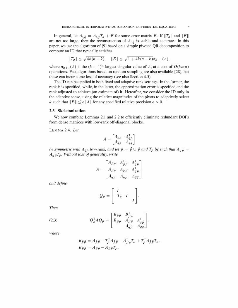
COROLLARY 2.3. Let A D AW;q be a low-rank matrix. If q D yq [ Lq and Tq aresuch that AW; Lq D AW;yqTq , then�
In general, let AW; Lq D AW;yqTq C E for some error matrix E. If kTqk and kEkare not too large, then the reconstruction of AW; Lq is stable and accurate. In thispaper, we use the algorithm of [9] based on a simple pivoted QR decomposition tocompute an ID that typically satisfies
kTqk �p4k.n � k/; kEk �
p1C 4k.n � k/�kC1.A/;
where �kC1.A/ is the .k C 1/st largest singular value of A, at a cost of O.kmn/operations. Fast algorithms based on random sampling are also available [28], butthese can incur some loss of accuracy (see also Section 4.5).
The ID can be applied in both fixed and adaptive rank settings. In the former, therank k is specified, while, in the latter, the approximation error is specified and therank adjusted to achieve (an estimate of) it. Hereafter, we consider the ID only inthe adaptive sense, using the relative magnitudes of the pivots to adaptively selectk such that kEk . �kAk for any specified relative precision � > 0.
2.3 SkeletonizationWe now combine Lemmas 2.1 and 2.2 to efficiently eliminate redundant DOFs
from dense matrices with low-rank off-diagonal blocks.
LEMMA 2.4. Let
A D
�App AT
qp
Aqp Aqq
�be symmetric with Aqp low-rank, and let p D yp [ Lp and Tp be such that Aq Lp DAq ypTp. Without loss of generality, write
A D
264A Lp Lp ATyp Lp
ATq Lp
A yp Lp A yp yp ATq yp
Aq Lp Aq yp Aqq
375and define
Qp D
24 I
�Tp I
I
35:Then
QTpAQp D
24B Lp Lp BTyp Lp
B yp Lp A yp yp ATq yp
Aq yp Aqq
35;(2.3)
where
B Lp Lp D A Lp Lp � TTpA yp Lp � A
Typ LpTp C T
TpA yp ypTp;
B yp Lp D A yp Lp � A yp ypTp;
8 K. L. HO AND L. YING
so
STLpQTpAQpS Lp D
24D Lp B yp yp ATq yp
Aq yp Aqq
35 � Zp.A/;(2.4)
where S Lp is the elimination operator of Lemma 2.1 associated with Lp and B yp yp DA yp yp � B yp LpB
�1Lp LpBTyp Lp
, assuming that B Lp Lp is nonsingular.
In essence, the ID sparsifies A by decoupling Lp from q, thereby allowing itto be eliminated by using efficient sparse techniques. We refer to this procedureas skeletonization since only the skeletons yp remain. Note that the interactionsinvolving q D pc are unchanged. A very similar approach has previously beendescribed in the context of HSS Cholesky decompositions [45] by combining thestructure-preserving rank-revealing factorization [46] with reduced matrices [42].
In general, the ID often only approximately sparsifies A (for example, if its off-diagonal blocks are low-rank only to a specified numerical precision) so that (2.3)and consequently (2.4) need not hold exactly. In such cases, the skeletonizationoperator Zp.�/ should be interpreted as also including an intermediate truncationstep that enforces sparsity explicitly. For notational convenience, however, we willcontinue to identify the left- and right-hand sides of (2.4) by writing Zp.A/ �STLpQTpAQpS Lp, with the truncation to be understood implicitly.
In this paper, we often work with a collection C of disjoint index sets, whereAc;cc and Acc;c are numerically low-rank for all c 2 C . Applying Lemma 2.4 toall c 2 C gives
ZC .A/ � UTAU; U D
Yc2C
QcS Lc ;
where the redundant DOFs Lc for each c 2 C have been decoupled from the rest andthe matrix product over C can be taken in any order. The resulting skeletonizedmatrix ZC .A/ is significantly sparsified and has a block diagonal structure overthe index groups
� D�[c2C
f Lcg�[
ns n
[c2C
Lco:
3 Multifrontal FactorizationIn this section, we review MF, which constructs a multilevel LDL decomposition
of A by using Lemma 2.1 to eliminate DOFs according to a hierarchical sequenceof domain separators. Our presentation will tend to emphasize its geometric as-pects [15]; more algebraic treatments can be found in [12, 33].
We begin with a detailed description of MF in 2D before extending to 3D in thenatural way. The same presentation framework will also be used for HIF-DE inSection 4, which we hope will help make clear the specific innovations responsiblefor its improved complexity estimates.
FIGURE 3.1. Active DOFs at each level ` of MF in 2D.
3.1 Two DimensionsConsider the PDE (1.1) on � D .0; 1/2 with zero Dirichlet boundary condi-
tions, discretized using finite differences via the five-point stencil over a uniformn � n grid for simplicity. More general domains, boundary conditions, and dis-cretizations can be handled without difficulty, but the current setting will serve tofix ideas. Let h be the step size in each direction and assume that n D 1=h D 2Lm,wherem D O.1/ is a small integer. Integer pairs j D .j1; j2/ index the grid pointsxj D hj D h.j1; j2/ for 1 � j1; j2 � n � 1. The discrete system (1.2) then reads
�1
h2.aj�e1=2 C ajCe1=2 C aj�e2=2 C ajCe2=2/uj
�1
h2
�aj�e1=2uj�e1
C ajCe1=2ujCe1
C aj�e2=2uj�e2C ajCe2=2ujCe2
�C bjuj D fj
at each xj , where aj D a.hj / is sampled on the “staggered” dual grid for e1 D.1; 0/ and e2 D .0; 1/ the unit coordinate vectors, bj D b.xj /, fj D f .xj /, anduj is the approximation to u.xj /. The resulting matrix A is sparse and symmetric,consisting only of nearest-neighbor interactions. The total number of DOFs isN D .n � 1/2, each of which is associated with a point xj and an index in s.
The algorithm proceeds by eliminating DOFs level by level. At each level `,the set of DOFs that have not been eliminated are called active with indices s`.Initially, we set A0 D A and s0 D s. Figure 3.1 shows the active DOFs at eachlevel for a representative example.
Level 0
Defined at this stage are A0 and s0. Partition � by 1D separators mh.j1; � /and mh.�; j2/ for 1 � j1; j2 � 2L � 1 every mh D n=2L units in each directioninto interior square cells mh.j1 � 1; j1/ � mh.j2 � 1; j2/ for 1 � j1; j2 � 2L.Observe that distinct cells do not interact with each other since they are bufferedby the separators. Let C0 be the collection of index sets corresponding to the activeDOFs of each cell. Then elimination with respect to C0 gives
A1 D WT0 A0W0; W0 D
Yc2C0
Sc ;
10 K. L. HO AND L. YING
where the DOFsSc2C0
c have been eliminated (and marked inactive). Let s1 Ds0 n
Sc2C0
c be the remaining active DOFs. The matrix A1 is block diagonal withblock partitioning
�1 D� [c2C0
fcg�[ fs1g:
Level `
Defined at this stage are A` and s`. Partition � by 1D separators 2`mh.j1; � /and 2`mh. � ; j2/ for 1 � j1; j2 � 2L�` � 1 every 2`mh D n=2L�` units ineach direction into interior square cells 2`mh.j1 � 1; j1/ � 2`mh.j2 � 1; j2/ for1 � j1; j2 � 2L�`. Let C` be the collection of index sets corresponding to theactive DOFs of each cell. Elimination with respect to C` then gives
A`C1 D WT` A`W`; W` D
Yc2C`
Sc ;
where the DOFsSc2C`
c have been eliminated. The matrix A`C1 is block diago-nal with block partitioning
�`C1 D� [c2C0
fcg�[ � � � [
� [c2C`
fcg�[ fs`C1g;
where s`C1 D s` nSc2C`
c.
Level L
Finally, we have AL and sL, where D � AL is block diagonal with blockpartitioning
�L D� [c2C0
fcg�[ � � � [
� [c2CL�1
fcg�[ fsLg:
Combining over all levels gives
D D W TL�1 � � �W
T0 AW0 � � �WL�1;
where eachW` is a product of unit upper triangular matrices, each of which can beinverted simply by negating its off-diagonal entries. Therefore,
A D W �T0 � � �W
�TL�1DW
�1L�1 � � �W
�10 � F;(3.1a)
A�1 D W0 � � �WL�1D�1W T
L�1 � � �WT0 D F
�1:(3.1b)
The factorization F is an LDL decomposition of A that is numerically exact (tomachine precision, up to conditioning), whose inverse F�1 can be applied as a fastdirect solver. Clearly, if A is SPD, then so are F and F�1; in this case, F can, infact, be written as a Cholesky decomposition by storing D in Cholesky form. Weemphasize that F and F�1 are not assembled explicitly and are used only in theirfactored representations.
The entire procedure is summarized compactly as Algorithm 3.1. In general,we can construct the cell partitioning at each level using an adaptive quadtree [38],
which recursively subdivides the domain until each node contains onlyO.1/DOFs,provided that some appropriate postprocessing is done to define “thin” separatorsin order to optimally exploit sparsity (see Section 4.5).
Algorithm 3.1 MF.A0 D A F initializefor ` D 0; 1; : : : ; L � 1 do F loop from finest to coarsest level
A`C1 D WT`A`W` F eliminate interior cells
end forA D W �T
0 � � �W�TL�1ALW
�1L�1 � � �W
�10 F LDL decomposition
3.2 Three DimensionsConsider now the analogous setting in 3D, where � D .0; 1/3 is discretized
using the seven-point stencil over a uniform n� n� n mesh with grid points xj Dhj D h.j1; j2; j3/ for j D .j1; j2; j3/:
1
h2.aj�e1=2 C ajCe1=2 C aj�e2=2 C ajCe2=2 C aj�e3=2 C ajCe3=2/uj
�1
h2
�aj�e1=2uj�e1
C ajCe1=2ujCe1C aj�e2=2uj�e2
C ajCe2=2ujCe2
C aj�e3=2uj�e3C ajCe3=2ujCe3
�C bjuj D fj ;
where e1 D .1; 0; 0/, e2 D .0; 1; 0/, and e3 D .0; 0; 1/. The total number of DOFsis N D .n � 1/3.
The algorithm extends in the natural way with 2D separators 2`mh.j1; � ; � /,2`mh. � ; j2; � /, and 2`mh. � ; � ; j3/ for 1 � j1; j2; j3 � 2L�` � 1 every 2`mh Dn=2L�` units in each direction now partitioning � into interior cubic cells
2`mh.j1 � 1; j1/ � 2`mh.j2 � 1; j2/ � 2
`mh.j3 � 1; j3/
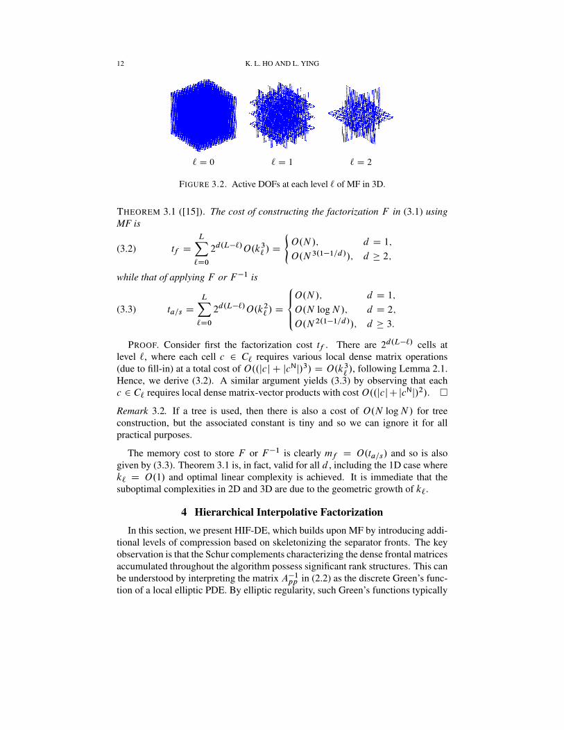
at level ` for 1 � j1; j2; j3 � 2L�`. With this modification, the rest of the al-gorithm remains unchanged. Figure 3.2 shows the active DOFs at each level fora representative example. The output is again a factorization of the form (3.1).General geometries can be treated using an adaptive octree.
3.3 Complexity EstimatesWe next analyze the computational complexity of MF. This is determined by
the size jcj of a typical index set c 2 C`, which we write as k` D O.2.d�1/`/
following the separator structure. Note furthermore that jcNj D O.k`/ as wellsince cN is restricted to the separators enclosing the DOFs c.
12 K. L. HO AND L. YING
` D 0 ` D 1 ` D 2
FIGURE 3.2. Active DOFs at each level ` of MF in 3D.
THEOREM 3.1 ([15]). The cost of constructing the factorization F in (3.1) usingMF is
tf D
LX`D0
2d.L�`/O.k3` / D
(O.N/; d D 1;
O.N 3.1�1=d//; d � 2;(3.2)
while that of applying F or F�1 is
ta=s D
LX`D0
2d.L�`/O.k2` / D
8<:O.N/; d D 1;
O.N logN/; d D 2;
O.N 2.1�1=d//; d � 3:
(3.3)
PROOF. Consider first the factorization cost tf . There are 2d.L�`/ cells atlevel `, where each cell c 2 C` requires various local dense matrix operations(due to fill-in) at a total cost of O..jcj C jcNj/3/ D O.k3
`/, following Lemma 2.1.
Hence, we derive (3.2). A similar argument yields (3.3) by observing that eachc 2 C` requires local dense matrix-vector products with costO..jcjCjcNj/2/. �
Remark 3.2. If a tree is used, then there is also a cost of O.N logN/ for treeconstruction, but the associated constant is tiny and so we can ignore it for allpractical purposes.
The memory cost to store F or F�1 is clearly mf D O.ta=s/ and so is alsogiven by (3.3). Theorem 3.1 is, in fact, valid for all d , including the 1D case wherek` D O.1/ and optimal linear complexity is achieved. It is immediate that thesuboptimal complexities in 2D and 3D are due to the geometric growth of k`.
4 Hierarchical Interpolative FactorizationIn this section, we present HIF-DE, which builds upon MF by introducing addi-
tional levels of compression based on skeletonizing the separator fronts. The keyobservation is that the Schur complements characterizing the dense frontal matricesaccumulated throughout the algorithm possess significant rank structures. This canbe understood by interpreting the matrix A�1pp in (2.2) as the discrete Green’s func-tion of a local elliptic PDE. By elliptic regularity, such Green’s functions typically
have numerically low-rank off-diagional blocks. The same rank structure essen-tially carries over to the Schur complement Bqq itself, as indeed has previouslybeen recognized and successfully exploited [1, 2, 16, 17, 20, 34, 39, 40, 42–44].
The interaction ranks of the Schur complement interactions (SCIs) constitutingBqq have been the subject of several analytic studies [4–6, 8], though none haveconsidered the exact type with which we are concerned in this paper. Such ananalysis, however, is not our primary goal, and we will be content simply with anempirical description. In particular, we have found through extensive numericalexperimentation (Section 5) that standard multipole estimates [22, 23] appear tohold for SCIs. We hereafter take this as an assumption, from which we can expectthat the skeletons of a given cluster of DOFs will tend to lie along its boundary[30, 31], thus exhibiting a dimensional reduction.
We are now in a position to motivate HIF-DE. Considering the 2D case forconcreteness, the main idea is simply to employ an additional level `C 1
2of edge
skeletonization after each level ` of interior cell elimination. This fully exploitsthe 1D geometry of the active DOFs and effectively reduces each front to 0D. Ananalogous strategy is adopted in 3D for reduction to either 1D by skeletonizingcubic faces or to 0D by skeletonizing faces then edges. In principle, the latter ismore efficient but can generate fill-in and so must be used with care.
The overall approach of HIF-DE is closely related to that of [2,16,17,20,39,40,44], but our sparsification framework permits a much simpler implementation andanalysis. As with MF, we begin first in 2D before extending to 3D.
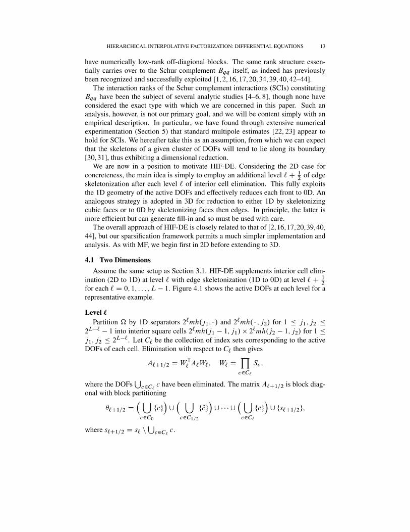
4.1 Two DimensionsAssume the same setup as Section 3.1. HIF-DE supplements interior cell elim-
ination (2D to 1D) at level ` with edge skeletonization (1D to 0D) at level ` C 12
for each ` D 0; 1; : : : ; L � 1. Figure 4.1 shows the active DOFs at each level for arepresentative example.
Level `
Partition � by 1D separators 2`mh.j1; � / and 2`mh. � ; j2/ for 1 � j1; j2 �
L�`. Let C` be the collection of index sets corresponding to the activeDOFs of each cell. Elimination with respect to C` then gives
A`C1=2 D WT` A`W`; W` D
Yc2C`
Sc ;
where the DOFsSc2C`
c have been eliminated. The matrix A`C1=2 is block diag-onal with block partitioning
�`C1=2 D� [c2C0
fcg�[
� [c2C1=2
f Lcg�[ � � � [
� [c2C`
fcg�[ fs`C1=2g;
where s`C1=2 D s` nSc2C`
c.
14 K. L. HO AND L. YING
` D 0 ` D 12
` D 1 ` D 3=2
` D 2 ` D 5=2 ` D 3
FIGURE 4.1. Active DOFs at each level ` of HIF-DE in 2D.
Level ` C12
Partition � into Voronoi cells [3] about the edge centers 2`mh.j1; j2 � 12/ for
1 � j1 � 2L�` � 1, 1 � j2 � 2L�` and 2`mh.j1 � 1
2; j2/ for 1 � j1 � 2L�`,
1 � j2 � 2L�` � 1. Let C`C1=2 be the collection of index sets corresponding to
the active DOFs of each cell. Skeletonization with respect to C`C1=2 then gives
A`C1 D ZC`C1=2.A`C1=2/ � U
T`C1=2A`C1=2U`C1=2;
U`C1=2 DY
c2C`C1=2
QcS Lc ;
where the DOFsSc2C`C1=2
Lc have been eliminated. Note that no fill-in is gener-ated since the DOFs yc for each c 2 C`C1=2 are already connected via SCIs fromelimination at level `. The matrix A`C1 is block diagonal with block partitioning
This is a factorization very similar to that in (3.1) except(1) it has twice as many factors,(2) it is now an approximation, and(3) the skeletonization matrices U` are composed of both upper and lower tri-
angular factors and so are not themselves triangular (but are still easilyinvertible).
We call (4.2) an approximate generalized LDL decomposition, with F�1 servingas a direct solver at high accuracy or as a preconditioner otherwise.
Unlike MF, if A is SPD, then D and hence F now only approximate SPD ma-trices. The extent of this approximation is governed by Weyl’s inequality.
THEOREM 4.1. If A;B 2 RN�N are symmetric, then
j�i .A/ � �i .B/j � kA � Bk; i D 1; 2; : : : ; N;
where �i .�/ returns the i th largest eigenvalue of a symmetric matrix.
COROLLARY 4.2. If A is SPD with F D ACE symmetric such that kEk � �kAkfor ��.A/ < 1, where �.A/ D kAkkA�1k is the condition number of A, then F isSPD.
PROOF. By Theorem 4.1, j�i .A/ � �i .F /j � kEk D �kAk for all i D 1; 2;
: : : ; N , so ˇ�i .A/ � �i .F /
�i .A/
ˇ�
ˇ�i .A/ � �i .F /
�N .A/
ˇ� �kAkkA�1k D ��.A/:(4.3)
This implies that �i .F / � .1 � ��.A// �i .A/, so �i .F / > 0 if ��.A/ < 1 since�i .A/ > 0 by assumption. �
Remark 4.3. Equation (4.3) actually proves a much more general result, namelythat all eigenvalues are approximated to relative precision ��.A/.
The requirement that ��.A/ < 1 is necessary for F�1 to achieve any accuracywhatsoever and hence is quite weak. Therefore, F is SPD under very mild condi-tions, in which case (4.2) can be interpreted as a generalized Cholesky decomposi-tion. Its inverse F�1 is then also SPD and can be used, e.g., as a preconditioner inCG.
The entire procedure is summarized as Algorithm 4.1.
16 K. L. HO AND L. YING
Algorithm 4.1 HIF-DE.A0 D A F initializefor ` D 0; 1; : : : ; L � 1 do F loop from finest to coarsest level
A`C1=2 D WT`A`W` F eliminate interior cells
A`C1 D ZC`C1=2.A`C1=2/ � U
T`C1=2
A`C1=2U`C1=2 F skeletonize edges(faces)
end forA � V �T
0 V �T1=2� � �V �T
L�1=2ALV
�1L�1=2
� � �V �11=2V �10 F generalized LDL
decomposition
` D 0 ` D 12
` D 1
` D 32
` D 2
FIGURE 4.2. Active DOFs at each level ` of HIF-DE in 3D.
4.2 Three DimensionsAssume the same setup as in Section 3.2. There are two variants of HIF-DE in
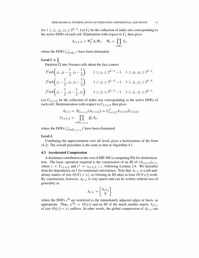
3D: a direct generalization of the 2D algorithm by combining interior cell elimi-nation (3D to 2D) with face skeletonization (2D to 1D) and a more complicatedversion adding also edge skeletonization (1D to 0D) afterward. We will continueto refer to the former simply as HIF-DE and call the latter “HIF-DE in 3D withedge skeletonization.” For unity of presentation, we will discuss only HIF-DEhere, postponing the alternative formulation until Section 4.5. Figure 4.2 showsthe active DOFs at each level for HIF-DE on a representative example.
for 1 � j1; j2; j3 � 2L�`. Let C` be the collection of index sets corresponding tothe active DOFs of each cell. Elimination with respect to C` then gives
A`C1=2 D WT` A`W`; W` D
Yc2C`
Sc ;
where the DOFsSc2C`
c have been eliminated.
Level ` C12
Partition � into Voronoi cells about the face centers
2`mh
�j1; j2 �
1
2; j3 �
1
2
�; 1 � j1 � 2
L�`� 1; 1 � j2; j3 � 2
L�`;
2`mh
�j1 �
1
2; j2; j3 �
1
2
�; 1 � j2 � 2
L�`� 1; 1 � j1; j3 � 2
L�`;
2`mh
�j1 �
1
2; j2 �
1
2; j3
�; 1 � j3 � 2
L�`� 1; 1 � j1; j2 � 2
L�`:
Let C`C1=2 be the collection of index sets corresponding to the active DOFs ofeach cell. Skeletonization with respect to C`C1=2 then gives
A`C1 D ZC`C1=2.A`C1=2/ � U
T`C1=2A`C1=2U`C1=2;
U`C1=2 DY
c2C`C1=2
QcS Lc ;
where the DOFsSc2C`C1=2
Lc have been eliminated.
Level L
Combining the approximation over all levels gives a factorization of the form(4.2). The overall procedure is the same as that in Algorithm 4.1.
4.3 Accelerated CompressionA dominant contribution to the cost of HIF-DE is computing IDs for skeletoniza-
tion. The basic operation required is the construction of an ID of .A`C1=2/cc;c ,where c 2 C`C1=2 and cc D s`C1=2 n c, following Lemma 2.4. We hereafterdrop the dependence on ` for notational convenience. Note that Acc;c is a tall-and-skinny matrix of size O.N/ � jcj, so forming its ID takes at least O.N jcj/ work.By construction, however, Acc;c is very sparse and can be written without loss ofgenerality as
Acc;c D
�AcN;c
0
�;
where the DOFs cN are restricted to the immediately adjacent edges or faces, asappropriate. Thus, jcNj D O.jcj/ and an ID of the much smaller matrix AcN;c
of size O.jcj/ � jcj suffices. In other words, the global compression of Acc;c can
18 K. L. HO AND L. YING
FIGURE 4.3. Accelerated compression by exploiting sparsity. In 2D,the number of neighboring edges (left) that must be included when skele-tonizing a given edge (gray outline) can be substantially reduced by re-stricting to only the interior DOFs of that edge (right). An analogoussetting applies for faces in 3D.
be performed via the local compression of AcN;c . This observation is critical forreducing the asymptotic complexity.
We can pursue further acceleration by optimizing jcNj as follows. Considerthe reference domain configuration depicted in Figure 4.3, which shows the activeDOFs s`C1=2 after interior cell elimination at level ` in 2D. The Voronoi parti-tioning scheme clearly groups together all interior DOFs of each edge, but thoseat the corner points 2`mh.j1; j2/ for 1 � j1; j2 � 2L�` � 1 are equidistant tomultiple Voronoi centers and can be assigned arbitrarily (or, in fact, not at all). Letc 2 C`C1=2 be a given edge and suppose that it includes both of its endpoints.Then its neighbor set cN includes all immediately adjacent edges as shown (left).But the only DOFs in c that interact with the edges to the left or right are preciselythe corresponding corner points. Therefore, we can reduce cN to only those edgesbelonging to the two cells on either side of the edge defining c by restricting to onlyits interior DOFs (right); i.e., we exclude from C`C1=2 all corner points. This canalso be interpreted as preselecting the corner points as skeletons (as must be thecase because of the sparsity pattern of Acc;c) and suitably modifying the remainingcomputation. In 2D, this procedure lowers the cost of the ID by about a factor of17=6 D 2:8333 : : : . In 3D, an analogous situation holds for faces with respect to“corner” edges and the cost is reduced by a factor of 37=5 D 7:4.
It is also possible to accelerate the ID using fast randomized methods [28] basedon compressing ˆcAcN;c , where ˆc is a small Gaussian random sampling matrix.However, we did not find a significant improvement in performance and so did notuse this optimization in our tests for simplicity (see also Section 4.5).
4.4 Optimal Low-Rank ApproximationAlthough we have built our algorithms around the ID, it is actually not essential
(at least with HIF-DE as presently formulated) and other low-rank approximationscan just as well be used. Perhaps the most natural of these is the singular valuedecomposition (SVD), which is optimal in the sense that it achieves the minimalapproximation error for a given rank [19]. Recall that the SVD of a matrix A 2Rm�n is a factorization of the formA D U†V T, whereU 2 Rm�m and V 2 Rn�n
are orthogonal, and † 2 Rm�n is diagonal with the singular values of A as itsentries. The following is the analogue of Corollary 2.3 using the SVD.
LEMMA 4.4. Let A 2 Rm�n with rank k � min.m; n/ and SVD
A D U†V TD�U1 U2
��0†2
��V1 V2
�T;
where †2 2 Rk�k . Then
U TA D †V TD
�0
†2VT2
�; AV D U† D
�0 U2†2
�:
The analogue of Lemma 2.4 is then the following:
LEMMA 4.5. Let
A D
�App AT
qp
Aqp Aqq
�be symmetric for Aqp low-rank with SVD
Aqp D Apc;p D Up†pVTp D
�Up;1 Up;2
��0†p;2
��Vp;1 Vp;2
�T:
If Qp D diag.Vp; I /, then
(4.4)
QTpAQp D
24 V Tp AppVp
�0
†p;2UTp;2
��0 Up;2†p;2
�Aqq
35�
24Bp1;p1BTp2;p1
Bp2;p1Bp2;p2
†p;2UTp;2
Up;2†p;2 Aqq
35on conformably partitioning p D p1 [ p2, so
STp1QTpAQpSp1
D
24Dp1
zBp2;p2†p;2U
Tp;2
Up;2†p;2 Aqq
35;where Sp1
is the elimination operator of Lemma 2.1 associated with p1 and
zBp2;p2D Bp2;p2
� Bp2;p1B�1p1;p1
BTp2;p1
;
where we assume that Bp1;p1is nonsingular.
The external interactions Up;2†p;2 with the SVD “skeletons” p2 are a linearcombination of the original external interactions Aqp involving all of p. Thus, theDOFs p2 are, in a sense, delocalized across all points associated with p, thoughthey can still be considered to reside on the separators.
The primary advantages of using the SVD over the ID are that (1) it can achievebetter compression since a smaller rank may be required for any given precision
20 K. L. HO AND L. YING
(A) Face skeletonization. (B) Edge configuration from top viewat interior slice.
FIGURE 4.4. Loss of sparsity from edge skeletonization in 3D. Faceskeletonization (left) typically leaves several layers of DOFs along theperimeter, which lead to thick edges (right) that connect DOFs acrosscubic cell boundaries upon skeletonization (3 � 3 grid of cells shown inexample with a thick edge outlined in gray).
and (2) the sparsification matrix Qp in (4.4) is orthogonal, which provides im-proved numerical stability, especially when used in a multilevel setting such as(4.2). However, there are several disadvantages as well, chief among them:
� the extra computational cost, which typically is about 2 to 3 times larger;� the need to overwrite matrix entries involving the index set q in (4.4),
which we remark is still sparse; and� the loss of precise geometrical information associated with each DOF.
Of these, the last is arguably the most important since it destroys the dimensionalreduction interpretation of HIF-DE, which is crucial for achieving estimatedO.N/complexity in 3D, as we shall see next.
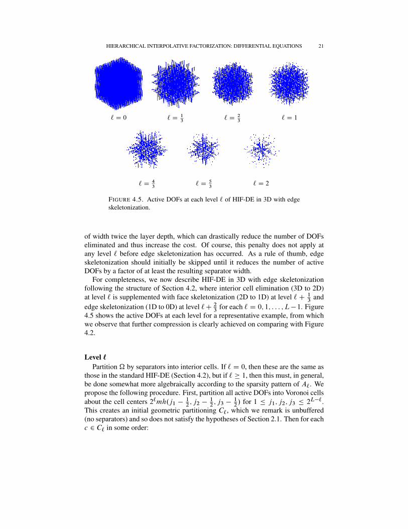
4.5 Three-Dimensional Variant with Edge SkeletonizationIn Section 4.2, we presented a “basic” version of HIF-DE in 3D based on interior
cell elimination and face skeletonization, which from Figure 4.2 is seen to retainactive DOFs only on the edges of cubic cells. All fronts are hence reduced to 1D,which yields estimated O.N logN/ complexity for the algorithm (Section 4.6).Here, we seek to further accelerate this to O.N/ by skeletonizing each cell edgeand reducing it completely to 0D, as guided by our assumptions on SCIs. How-ever, a complication now arises in that fill-in can occur, which can be explained asfollows.
Consider the 3D problem and suppose that both interior cell elimination and faceskeletonization have been performed. Then as noted in Section 4.3, the remainingDOFs with respect to each face will be those on its boundary edges plus a fewinterior layers near the edges (Figure 4.4(A)) (the depth of these layers depends onthe compression tolerance �). Therefore, grouping the active DOFs by cell edgegives “thick” edges consisting not only of the DOFs on the edges themselves butalso those in the interior layers in the four transverse directions surrounding eachedge (Figure 4.4(B)). Skeletonizing these thick edges then generates SCIs actingon the skeletons of each edge group by Lemma 2.4, which generally causes DOFsto interact across cubic cell boundaries. The consequence of this is that the nextlevel of interior cell elimination must take into account, in effect, thick separators
FIGURE 4.5. Active DOFs at each level ` of HIF-DE in 3D with edgeskeletonization.
of width twice the layer depth, which can drastically reduce the number of DOFseliminated and thus increase the cost. Of course, this penalty does not apply atany level ` before edge skeletonization has occurred. As a rule of thumb, edgeskeletonization should initially be skipped until it reduces the number of activeDOFs by a factor of at least the resulting separator width.
For completeness, we now describe HIF-DE in 3D with edge skeletonizationfollowing the structure of Section 4.2, where interior cell elimination (3D to 2D)at level ` is supplemented with face skeletonization (2D to 1D) at level `C 1
3and
edge skeletonization (1D to 0D) at level `C 23
for each ` D 0; 1; : : : ; L�1. Figure4.5 shows the active DOFs at each level for a representative example, from whichwe observe that further compression is clearly achieved on comparing with Figure4.2.
Level `
Partition � by separators into interior cells. If ` D 0, then these are the same asthose in the standard HIF-DE (Section 4.2), but if ` � 1, then this must, in general,be done somewhat more algebraically according to the sparsity pattern of A`. Wepropose the following procedure. First, partition all active DOFs into Voronoi cellsabout the cell centers 2`mh.j1 � 1
2; j2 �
12; j3 �
12/ for 1 � j1; j2; j3 � 2L�`.
This creates an initial geometric partitioning C`, which we remark is unbuffered(no separators) and so does not satisfy the hypotheses of Section 2.1. Then for eachc 2 C` in some order:
22 K. L. HO AND L. YING
(1) Let
cED fi 2 c W .A`/cc;i ¤ 0g; cc
D
� [c02C`
c0�n c
be the set of indices of the DOFs in c with external interactions.(2) Replace c by c n cE in C`.
On termination, this process produces a collection C` of interior cells with minimalseparators adaptively constructed. Elimination with respect to C` then gives
A`C1=3 D WT` A`W`; W` D
Yc2C`
Sc ;
where the DOFsSc2C`
c have been eliminated.
Level ` C13
Partition � into Voronoi cells about the face centers
2`mh
�j1; j2 �
1
2; j3 �
1
2
�; 1 � j1 � 2
L�`� 1; 1 � j2; j3 � 2
L�`;
2`mh
�j1 �
1
2; j2; j3 �
1
2
�; 1 � j2 � 2
L�`� 1; 1 � j1; j2 � 2
L�`;
2`mh
�j1 �
1
2; j2 �
1
2; j3
�; 1 � j3 � 2
L�`� 1; 1 � j1; j2 � 2
L�`:
Let C`C1=3 be the collection of index sets corresponding to the active DOFs ofeach cell. Skeletonization with respect to C`C1=3 then gives
A`C2=3 D ZC`C1=3.A`C1=3/ � U
T`C1=3A`C1=3U`C1=3;
U`C1=3 DY
c2C`C1=3
QcS Lc ;
where the DOFsSc2C`C1=3
Lc have been eliminated.
Level ` C23
Partition � into Voronoi cells about the edge centers
Let C`C2=3 be the collection of index sets corresponding to the active DOFs ofeach cell. Skeletonization with respect to C`C2=3 then gives
A`C1 D ZC`C2=3.A`C2=3/ � U
T`C2=3A`C2=3U`C2=3;
U`C2=3 DY
c2C`C2=3
QcS Lc ;
where the DOFsSc2C`C2=3
Lc have been eliminated.
Level L
Combining the approximation over all levels gives
D � AL � VTL�1=3 � � �V
T2=3V
T1=3V
T0 AV0V1=3V2=3 � � �VL�1=3;
where V` is as defined in (4.1), so
A � V �T0 V �T
1=3V�T2=3 � � �V
�TL�1=3DV
�1L�1=3 � � �V
�12=3V
�11=3V
�10 � F;(4.5a)
A�1 � V0V1=3V2=3 � � �VL�1=3D�1V T
L�1=3 � � �VT2=3V
T1=3V
T0 D F
�1:(4.5b)
As in Section 4.1, if A is SPD, then so are F and F�1 provided that very mildconditions hold. We summarize the overall scheme as Algorithm 4.2.
Algorithm 4.2 HIF-DE in 3D with edge skeletonization.A0 D A F initializefor ` D 0; 1; : : : ; L � 1 do F loop from finest to coarsest level
A`C1=3 D WT`A`W` F eliminate interior cells
A`C2=3 D ZC`C1=3.A`C1=3/ � U
T`C1=3
A`C1=3U`C1=3 F skeletonize facesA`C1 D ZC`C2=3
.A`C2=3/ � UT`C2=3
A`C2=3U`C2=3 F skeletonize edgesend forA � V �T
0 V �T1=3� � �V �T
L�1=3DV �1
L�1=3� � �V �1
1=3V �10 F generalized LDL
decomposition
Unlike for the standard HIF-DE, randomized methods (Section 4.3) now tend tobe inaccurate when compressing SCIs. This could be remedied by considering in-stead ˆc.AcN;cA
TcN;c
/ AcN;c for some small integer D 1; 2; : : : , but the expenseof the extra multiplications usually outweighed any efficiency gains.
4.6 Complexity EstimatesWe now investigate the computational complexity of HIF-DE. For this, we need
to estimate the skeleton size jycj for a typical index set c 2 C` at fractional level `.This is determined by the rank behavior of SCIs, which we assume satisfy standardmultipole estimates [22, 23] as motivated by experimental observations. Then itcan be shown [30, 31] that the typical skeleton size is
k` D
(O.`/; ı D 1;
O.2.ı�1/`/; ı � 2;(4.6)
24 K. L. HO AND L. YING
where ı is the intrinsic dimension of a typical DOF cluster at level `, i.e., ı D 1 foredges (2D and 3D) and ı D 2 for faces (3D only). Note that we have suggestivelyused the same notation as for the index set size jcj in Section 3.3, which can bejustified by recognizing that the active DOFs c 2 C` for any ` are obtained bymerging skeletons from at most one integer level prior. We emphasize that (4.6)has yet to be proven, so all following results should formally be understood asconjectures, albeit ones with strong numerical support (Section 5).
THEOREM 4.6. Assume that (4.6) holds. Then the costs of constructing the fac-torization F in (4.2) or (4.5) using HIF-DE with accelerated compression and ofapplying F or F�1 are, respectively, tf ; ta=s D O.N/ in 2D; tf D O.N logN/and ta=s D O.N/ in 3D; and tf ; ta=s D O.N/ in 3D with edge skeletonization.
PROOF. The costs of constructing and applying the factorization are clearly
tf D
LX0
`D0
O�2d.L�`/k3`
�; ta=s D
LX0
`D0
O�2d.L�`/k2`
�;
where prime notation denotes summation over all levels, both integer and frac-tional, and k` is as given by (4.6) for ı appropriately chosen. In 2D, all fronts arereduced to 1D edges, so ı D 1; in 3D, compression on 2D faces has ı D 2; and in3D with edge skeletonization, we again have ı D 1. The claim follows by directcomputation. �
5 Numerical ResultsIn this section, we demonstrate the efficiency of HIF-DE by reporting numerical
results for some benchmark problems in 2D and 3D. All algorithms and exampleswere implemented in MATLAB® and are freely available at https://github.com/klho/FLAM/. In what follows, we refer to MF as mf2 in 2D and mf3 in 3D.Similarly, we call HIF-DE hifde2 and hifde3, respectively, and denote by hifde3xthe 3D variant with edge skeletonization. All codes are fully adaptive and builton quadtrees in 2D and octrees in 3D. The average block size jcj at level 0 (andhence the tree depth L) was chosen so that roughly half of the initial DOFs areeliminated. In select cases, the first few fractional levels of HIF-DE were skippedto optimize the running time. Diagonal blocks, i.e., App in Lemma 2.1, werefactored using the Cholesky decomposition if A is SPD and the (partially pivoted)LDL decomposition otherwise.
For each example, the following are given:� �: relative precision of the ID;� N : total number of DOFs in the problem;� jsLj: number of active DOFs remaining at the highest level;� tf : wall clock time for constructing the factorization F in seconds;� mf : memory required to store F in GB;� ta=s: wall clock time for applying F or F�1 in seconds;
FIGURE 5.1. Scaling results for Example 1. Wall clock times tf (ı) andta=s (�) and storage requirementsmf (˘) are shown for mf2 (white) andhifde2 (black) at precision � D 10�9. Dotted lines denote extrapolatedvalues. Included also are reference scalings (gray dashed lines) ofO.N/and O.N 3=2/ (left, from bottom to top), and O.N/ and O.N logN/(right). The lines for ta=s (bottom left) lie nearly on top of each other.
� ea: a posteriori estimate of kA � F k=kAk (see below);� es: a posteriori estimate of kI � AF�1k � kA�1 � F�1k=kA�1k;� ni : number of iterations to solve (1.2) using CG [29, 41] (if SPD) or GM-
RES [37] with preconditioner F�1 to a tolerance of 10�12, where f is astandard uniform random vector.
We also compare against MF, which is numerically exact.The operator errors ea and es were estimated using power iteration with a stan-
dard uniform random start vector [11, 32] and a convergence criterion of 10�2 rel-ative precision in the matrix norm. This has a small probability of underestimatingthe error but seems to be quite robust in practice.
For simplicity, all PDEs were defined over � D .0; 1/d with (arbitrary) Dirich-let boundary conditions as in Section 3, discretized on a uniform n�n or n�n�nmesh using second-order central differences via the five-point stencil in 2D and theseven-point stencil in 3D.
All computations were performed in MATLAB® R2010b on a single core (with-out parallelization) of an Intel Xeon E7-4820 CPU at 2.0 GHz on a 64-bit Linuxserver with 256 GB of RAM.
5.1 Two DimensionsWe begin first in 2D, where we present three examples.
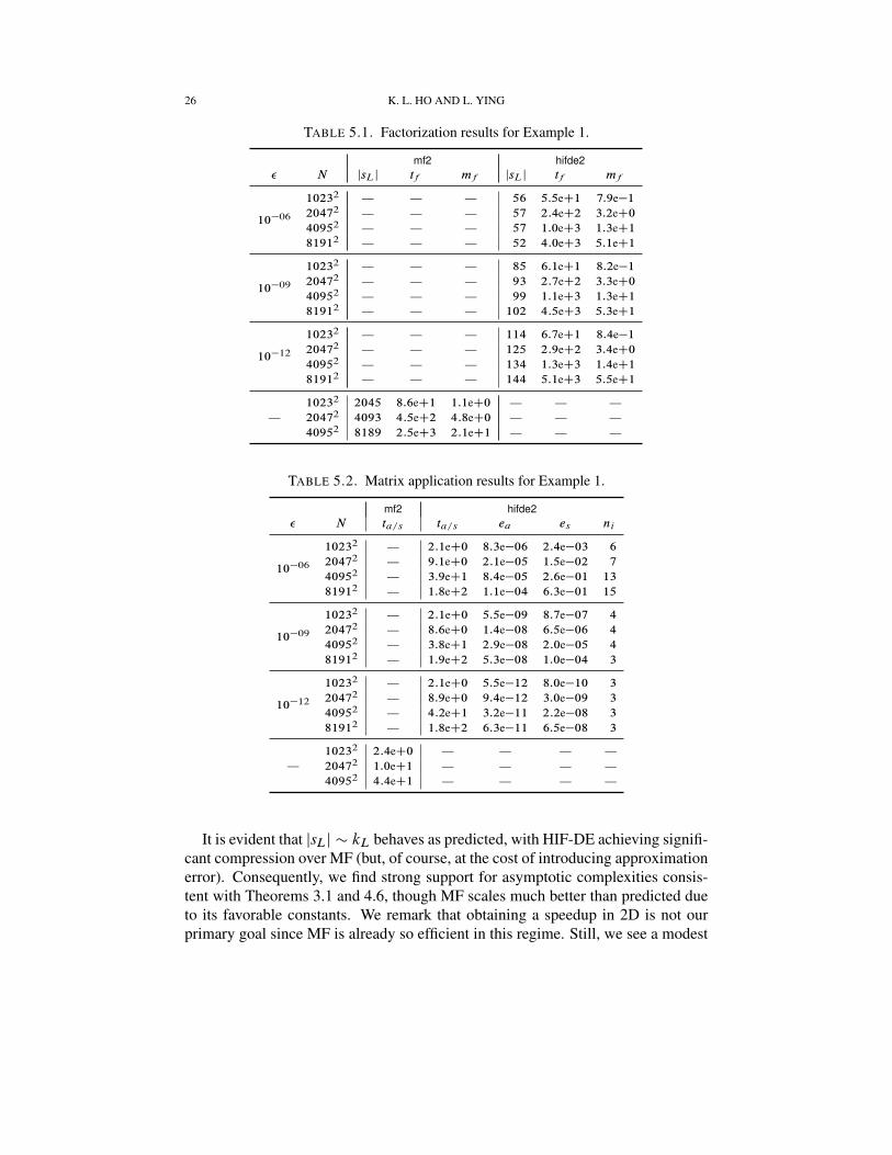
Example 1. Consider (1.1) with a.x/ � 1, b.x/ � 0, and � D .0; 1/2, i.e.,a simple Laplacian in the unit square. The resulting matrix A is SPD, which wefactored using both mf2 and hifde2 at � D 10�6, 10�9, and 10�12 (the compressiontolerances are for HIF-DE only). The data are summarized in Tables 5.1 and 5.2with scaling results shown in Figure 5.1.
It is evident that jsLj � kL behaves as predicted, with HIF-DE achieving signifi-cant compression over MF (but, of course, at the cost of introducing approximationerror). Consequently, we find strong support for asymptotic complexities consis-tent with Theorems 3.1 and 4.6, though MF scales much better than predicted dueto its favorable constants. We remark that obtaining a speedup in 2D is not ourprimary goal since MF is already so efficient in this regime. Still, we see a modest
FIGURE 5.2. Sample realization of a quantized high-contrast randomfield in 2D.
increase in performance and memory savings that allow us to run HIF-DE up toN D 81912, for which MF was not successful.
For all problem sizes tested, tf and mf are always smaller for HIF-DE, thoughta=s is quite comparable. This is because ta=s is dominated by memory access (atleast in our current implementation), which also explains its relative insensitivityto �. Furthermore, we observe that ta=s � tf for both methods, which makes themideally suited to systems involving multiple right-hand sides.
The forward approximation error ea D O.�/ for all N and seems to increaseonly mildly with N . This indicates that the local accuracy of the ID provides agood estimate of the overall accuracy of the algorithm, which is not easy to provesince the multilevel matrix factors constituting F are not orthogonal. On the otherhand, we expect the inverse approximation error to scale as es D O.�.A/ea/,where �.A/ D O.N/ for this example, and indeed we see that es is much largerdue to ill-conditioning. When using F�1 to precondition CG, however, the numberof iterations required is always very small. This indicates that F�1 is a highlyeffective preconditioner.
Example 2. Consider now the same setup as in Example 1 but with a.x/ a quan-tized high-contrast random field defined as follows:
(1) Initialize by sampling each staggered grid point aj from the standard uni-form distribution.
(2) Impose some correlation structure by convolving faj g with an isotropicGaussian of width 4h.
(3) Quantize by setting
aj D
(10�2; aj � �;
10C2; aj > �;
where � is the median of faj g.
Figure 5.2 shows a sample realization of such a high-contrast random field in 2D.The matrix A now has condition number �.A/ D O.�N/, where � D 104 isthe contrast ratio. Such high-contrast problems are typically extremely difficult to
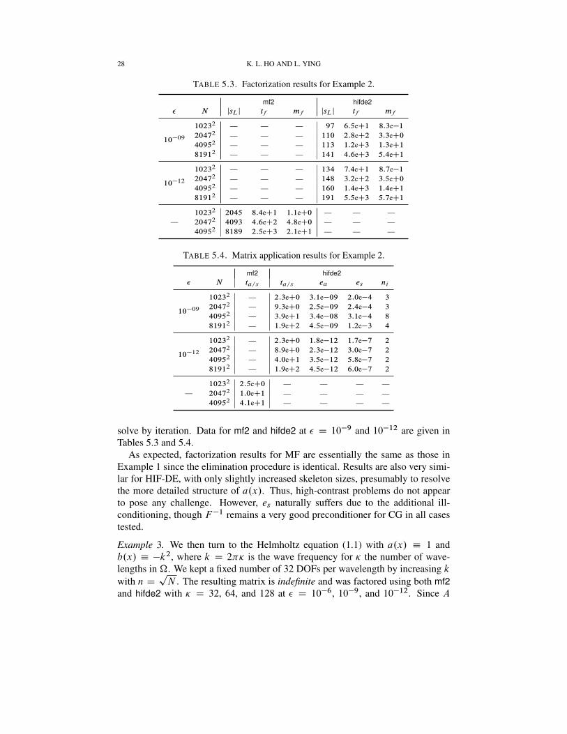
solve by iteration. Data for mf2 and hifde2 at � D 10�9 and 10�12 are given inTables 5.3 and 5.4.
As expected, factorization results for MF are essentially the same as those inExample 1 since the elimination procedure is identical. Results are also very simi-lar for HIF-DE, with only slightly increased skeleton sizes, presumably to resolvethe more detailed structure of a.x/. Thus, high-contrast problems do not appearto pose any challenge. However, es naturally suffers due to the additional ill-conditioning, though F�1 remains a very good preconditioner for CG in all casestested.
Example 3. We then turn to the Helmholtz equation (1.1) with a.x/ � 1 andb.x/ � �k2, where k D 2�� is the wave frequency for � the number of wave-lengths in �. We kept a fixed number of 32 DOFs per wavelength by increasing kwith n D
pN . The resulting matrix is indefinite and was factored using both mf2
and hifde2 with � D 32, 64, and 128 at � D 10�6, 10�9, and 10�12. Since A
is no longer SPD, F�1 now applies as a preconditioner for GMRES. The data aresummarized in Tables 5.5 and 5.6 with scaling results in Figure 5.3.
Overall, the results are very similar to those in Example 1 but with larger skele-ton sizes and some extra ill-conditioning of order O.k/. We remark, however, thatHIF-DE is effective only at low to moderate frequency since the rank structuresemployed break down as k ! 1. This can be understood by analogy with theHelmholtz Green’s function, whose off-diagonal blocks are full-rank in the limit(though other rank structures are possible [13, 14]). Indeed, we can already see anincreasing trend in jsLj beyond that observed in Examples 1 and 2. In the high-frequency regime, the only compression available is due to sparsity, with HIF-DE
30 K. L. HO AND L. YING
FIGURE 5.3. Scaling results for Example 3, comparing mf2 (white) withhifde2 (black) at precision � D 10�9; all other notation as in Figure 5.1.
essentially reducing to MF. Nonetheless, our results reveal no significant appar-ent failure and demonstrate that HIF-DE achieves linear complexity up to at least� � 102.
5.2 Three DimensionsWe next present three examples in 3D generalizing each of the 2D cases above.
Example 4. Consider the 3D analogue of Example 1, i.e., (1.1) with a.x/ � 1,b.x/ � 0, and � D .0; 1/3. Data for mf3, hifde3, and hifde3x at � D 10�3, 10�6,and 10�9 are given in Tables 5.7 and 5.8 with scaling results shown in Figure 5.4.
It is immediate that tf D O.N 2/ and ta=s D O.N 4=3/ for MF, which consider-ably degrades its performance for large N . Indeed, we were unable to run mf3 forN D 1273 because of the excessive memory cost. In contrast, HIF-DE scales muchbetter, with jsLj growing consistently with (4.6) for both variants. This providesstrong evidence for Theorem 4.6. However, the skeleton size is substantially largerthan in 2D, and neither hifde3 nor hifde3x quite achieve quasilinear complexity as
FIGURE 5.4. Scaling results for Example 4, comparing mf3 (white) withhifde3 (gray) and hifde3x (black) at precision � D 10�6. Includedalso are reference scalings of O.N/ and O.N 2/ (left), and O.N/ andO.N 4=3/ (right); all other notation as in Figure 5.1. The lines for hifde3and hifde3x lie nearly on top of each other; for tf (top left), they overlapalmost exactly.
predicted: the empirical scaling for tf for both algorithms at, e.g., � D 10�6 isapproximately O.N 1:4/. We believe this to be a consequence of the large interac-tion ranks, which make the asymptotic regime rather difficult to reach. In parallelwith Example 1, ea D O.�/ but es is somewhat larger due to ill-conditioning.We found F�1 to be a very effective preconditioner throughout. There were nosignificant differences in either computation time or accuracy between hifde3 andhifde3x, though the latter does provide some appreciable memory savings.
Example 5. Now consider the 3D analogue of Example 2, i.e., Example 4 but witha.x/ a quantized high-contrast random field as previously defined, extended to 3D
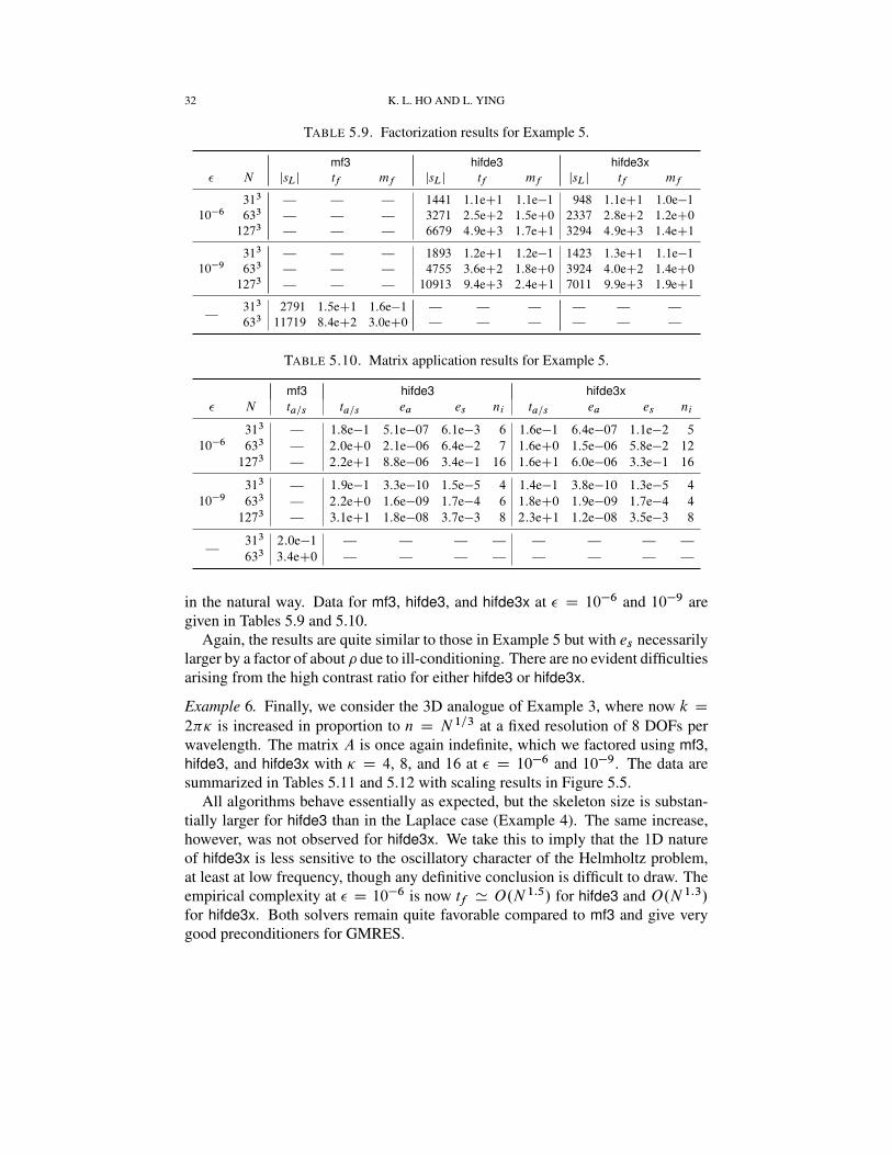
in the natural way. Data for mf3, hifde3, and hifde3x at � D 10�6 and 10�9 aregiven in Tables 5.9 and 5.10.
Again, the results are quite similar to those in Example 5 but with es necessarilylarger by a factor of about � due to ill-conditioning. There are no evident difficultiesarising from the high contrast ratio for either hifde3 or hifde3x.
Example 6. Finally, we consider the 3D analogue of Example 3, where now k D
2�� is increased in proportion to n D N 1=3 at a fixed resolution of 8 DOFs perwavelength. The matrix A is once again indefinite, which we factored using mf3,hifde3, and hifde3x with � D 4, 8, and 16 at � D 10�6 and 10�9. The data aresummarized in Tables 5.11 and 5.12 with scaling results in Figure 5.5.
All algorithms behave essentially as expected, but the skeleton size is substan-tially larger for hifde3 than in the Laplace case (Example 4). The same increase,however, was not observed for hifde3x. We take this to imply that the 1D natureof hifde3x is less sensitive to the oscillatory character of the Helmholtz problem,at least at low frequency, though any definitive conclusion is difficult to draw. Theempirical complexity at � D 10�6 is now tf ' O.N 1:5/ for hifde3 and O.N 1:3/
for hifde3x. Both solvers remain quite favorable compared to mf3 and give verygood preconditioners for GMRES.
FIGURE 5.5. Scaling results for Example 6, comparing mf3 (white) withhifde3 (gray) and hifde3x (black) at precision � D 10�6; all other nota-tion as in Figure 5.4.
6 Generalizations and ConclusionsIn this paper, we have introduced HIF-DE for the efficient factorization of dis-
cretized elliptic partial differential operators in 2D and 3D. HIF-DE combinesMF [12, 15, 33] with recursive dimensional reduction via frontal skeletonization to
34 K. L. HO AND L. YING
construct an approximate generalized LU/LDL decomposition at estimated quasi-linear cost. The latter enables significant compression over MF and is critical forimproving the asymptotic complexity, while the former is essential for optimallyexploiting sparsity and hence for achieving good practical performance. The result-ing factorization allows the rapid application of the matrix inverse, which providesa fast direct solver or preconditioner, depending on the accuracy. Furthermore,although we have focused here only on symmetric matrices, our techniques gen-eralize also to the unsymmetric case by defining analogous two-sided eliminationoperators Rp and Sp in (2.2) as in [31] and by compressing
Bc D
�AcN;c
Ac;cN
�instead of just AcN;c .
While we have reported numerical data only for PDEs with Dirichlet boundaryconditions, HIF-DE extends trivially to other types of boundary conditions as well.Preliminary tests with mixed Dirichlet-Neumann conditions reveal no discerniblechange in performance.
The skeletonization operator at the core of HIF-DE can be interpreted in severalways. For example, we can view it as an approximate local change of basis in orderto gain sparsity. Unlike traditional approaches, however, this basis is determinedoptimally on the fly using the ID. Skeletonization can also be regarded as adaptivenumerical upscaling or as implementing specialized restriction and prolongationoperators in the context of multigrid methods [7, 24, 47].
Although we have presently only considered sparse matrices arising from PDEs,the same basic approach can also be applied to structured dense matrices such asthose derived from the integral equation formulations of elliptic PDEs. This isdescribed in detail as algorithm HIF-IE in the companion paper [31], which usesskeletonization for all compression steps and likewise has quasilinear complexityestimates in both 2D and 3D. In particular, HIF-DE can be viewed as a heavilyspecialized version of HIF-IE by embedding it into the framework of MF in orderto exploit sparsity. The elimination operations in MF can also be seen as a trivialform of skeletonization acting on overlapping subdomains. Indeed, [31] showsthat recursive skeletonization [18, 21, 30, 35], a precursor of HIF-IE based on cellcompression, is essentially equivalent to MF.
Some important directions for future research include:
� Obtaining analytical estimates of the interaction rank for SCIs, even forthe simple case of the Laplacian. This would enable a much more preciseunderstanding of the complexity of HIF-DE, which has yet to be rigorouslyestablished.� Parallelizing HIF-DE, which, like MF, is organized according to a tree
structure where each node at a given level can be processed independentlyof the rest. In particular, the frontal matrices are now much more compact,
which should support better parallelization, and we anticipate that the over-all scheme will have significant impact on practical scientific computing.This is currently in active development.� Investigating alternative strategies for reducing skeleton sizes in 3D, which
can still be quite large, especially at high precision.� Understanding the extent to which our current techniques can be adapted to
highly indefinite problems, some of which have a Helmholtz character andpossess rank structures of a different type than that exploited here [13,14].Such problems can be very challenging to solve iteratively and present aprime target area for future fast direct solvers.
Acknowledgment. We would like to thank Jack Poulson for helpful discussions,Lenya Ryzhik for providing computing resources, and the anonymous referees fortheir careful reading of the manuscript, which have improved the paper tremen-dously. K.L.H. was partially supported by the National Science Foundation underaward DMS-1203554. L.Y. was partially supported by the National Science Foun-dation under award DMS-1328230 and the U.S. Department of Energy’s AdvancedScientific Computing Research program under award DE-FC02-13ER26134/DE-SC0009409.
Bibliography[1] Amestroy, P. R.; Ashcraft, C.; Boiteau, O.; Buttari, A.; L’Excellent, J.-Y.; Weisbecker, C. Im-
proving multifrontal methods by means of block low-rank representations. INPT-IRIT Techni-cal Report RT/APO/12/6; also appeared as INRIA Technical Report RR-8199, December 2012.SIAM J. Sci. Comput., submitted.
[2] Aminfar, A.; Ambikasaran, S.; Darve, E. A fast block low-rank dense solver with applicationsto finite-element matrices. Preprint, 2014. arXiv:1403.5337 [cs.NA]
[3] Aurenhammer, F. Voronoi diagrams—a survey of a fundamental geometric data structure. ACMComput. Surv. 23 (1991), no. 3, 345–405. doi:10.1145/116873.116880
[4] Bebendorf, M. Efficient inversion of the Galerkin matrix of general second-order elliptic op-erators with nonsmooth coefficients. Math. Comp. 74 (2005), no. 251, 1179–1199 (electronic).doi:10.1090/S0025-5718-04-01716-8
[5] Bebendorf, M.; Hackbusch, W. Existence of H -matrix approximants to the inverse FE-matrix of elliptic operators with L1-coefficients. Numer. Math. 95 (2003), no. 1, 1–28.doi:10.1007/s00211-002-0445-6
[6] Börm, S. Approximation of solution operators of elliptic partial differential equations by H -and H 2-matrices. Numer. Math. 115 (2010), no. 2, 165–193. doi:10.1007/s00211-009-0278-7
[7] Brandt, A. Multi-level adaptive solutions to boundary-value problems. Math. Comp. 31 (1977),no. 138, 333–390. doi:10.2307/2006422
[8] Chandrasekaran, S.; Dewilde, P.; Gu, M.; Somasunderam, N. On the numerical rank of the off-diagonal blocks of Schur complements of discretized elliptic PDEs. SIAM J. Matrix Anal. Appl.31 (2010), no. 5, 2261–2290. doi:10.1137/090775932
[9] Cheng, H.; Gimbutas, Z.; Martinsson, P. G.; Rokhlin, V. On the compression of low rank ma-trices. SIAM J. Sci. Comput. 26 (2005), no. 4, 1389–1404. doi:10.1137/030602678
[10] Davis, T. A. Direct methods for sparse linear systems. Fundamentals of Algo-rithms, 2. Society for Industrial and Applied Mathematics (SIAM), Philadelphia, 2006.doi:10.1137/1.9780898718881
[11] Dixon, J. D. Estimating extremal eigenvalues and condition numbers of matrices. SIAM J. Nu-mer. Anal. 20 (1983), no. 4, 812–814. doi:10.1137/0720053
[12] Duff, I. S.; Reid, J. K. The multifrontal solution of indefinite sparse symmetric linear equations.ACM Trans. Math. Software 9 (1983), no. 3, 302–325. doi:10.1145/356044.356047
[13] Engquist, B.; Ying, L. Fast directional multilevel algorithms for oscillatory kernels. SIAM J.Sci. Comput. 29 (2007), no. 4, 1710–1737 (electronic). doi:10.1137/07068583X
[14] Engquist, B.; Ying, L. A fast directional algorithm for high frequency acoustic scattering in twodimensions. Commun. Math. Sci. 7 (2009), no. 2, 327–345.
[15] George, A. Nested dissection of a regular finite element mesh. SIAM J. Numer. Anal. 10 (1973),345–363. doi:10.1137/0710032
[16] Gillman, A.; Martinsson, P. G. A direct solver with O.N/ complexity for variable coefficientelliptic PDEs discretized via a high-order composite spectral collocation method. SIAM J. Sci.Comput. 36 (2014), no. 4, A2023–A2046. doi:10.1137/130918988
[17] Gillman, A.; Martinsson, P.-G. AnO.N/ algorithm for constructing the solution operator to 2Delliptic boundary value problems in the absence of body loads. Adv. Comput. Math. 40 (2014),no. 4, 773–796. doi:10.1007/s10444-013-9326-z
[18] Gillman, A.; Young, P. M.; Martinsson, P.-G. A direct solver with O.N/ complexity for in-tegral equations on one-dimensional domains. Front. Math. China 7 (2012), no. 2, 217–247.doi:10.1007/s11464-012-0188-3
[19] Golub, G. H.; Van Loan, C. F. Matrix computations. Third edition. Johns Hopkins Studies inthe Mathematical Sciences. Johns Hopkins University Press, Baltimore, 1996.
[20] Grasedyck, L.; Kriemann, R.; Le Borne, S. Domain decomposition based H -LU precondition-ing. Numer. Math. 112 (2009), no. 4, 565–600. doi:10.1007/s00211-009-0218-6
[21] Greengard, L.; Gueyffier, D.; Martinsson, P.-G.; Rokhlin, V. Fast direct solvers for inte-gral equations in complex three-dimensional domains. Acta Numer. 18 (2009), 243–275.doi:10.1017/S0962492906410011
[22] Greengard, L.; Rokhlin, V. A fast algorithm for particle simulations. J. Comput. Phys. 73(1987), no. 2, 325–348. doi:10.1016/0021-9991(87)90140-9
[23] Greengard, L.; Rokhlin, V. A new version of the Fast Multipole Method for the Laplace equationin three dimensions. Acta Numerica 6 (1997), 229–269. doi:10.1017/S0962492900002725
[24] Hackbusch, W. Multigrid methods and applications. Springer Series in Computational Mathe-matics, 4. Springer, Berlin, 1985. doi:10.1007/978-3-662-02427-0
[25] Hackbusch, W. A sparse matrix arithmetic based on H -matrices. I. Introduction to H -matrices. Computing 62 (1999), no. 2, 89–108. doi:10.1007/s006070050015
[26] Hackbusch, W.; Börm, S. Data-sparse approximation by adaptive H 2-matrices. Computing 69(2002), no. 1, 1–35. doi:10.1007/s00607-002-1450-4
[27] Hackbusch, W.; Khoromskij, B. N. A sparse H -matrix arithmetic. II. Application to multi-dimensional problems. Computing 64 (2000), no. 1, 21–47.
[28] Halko, N.; Martinsson, P. G.; Tropp, J. A. Finding structure with randomness: probabilisticalgorithms for constructing approximate matrix decompositions. SIAM Rev. 53 (2011), no. 2,217–288. doi:10.1137/090771806
[29] Hestenes, M. R.; Stiefel, E. Methods of conjugate gradients for solving linear systems. J. Re-search Nat. Bur. Standards 49 (1952), 409–436 (1953).
[30] Ho, K. L.; Greengard, L. A fast direct solver for structured linear systems by recursive skele-tonization. SIAM J. Sci. Comput. 34 (2012), no. 5, A2507–A2532. doi:10.1137/120866683
[31] Ho, K. L.; Ying, L. Hierarchical interpolative factorization for elliptic operators: integral equa-tions. Comm. Pure Appl. Math., forthcoming.
[32] Kuczynski, J.; Wozniakowski, H. Estimating the largest eigenvalue by the power and Lanc-zos algorithms with a random start. SIAM J. Matrix Anal. Appl. 13 (1992), no. 4, 1094–1122.doi:10.1137/0613066
[33] Liu, J. W. H. The multifrontal method for sparse matrix solution: theory and practice. SIAMRev. 34 (1992), no. 1, 82–109. doi:10.1137/1034004
[34] Martinsson, P.-G. A fast direct solver for a class of elliptic partial differential equations. J. Sci.Comput. 38 (2009), no. 3, 316–330. doi:10.1007/s10915-008-9240-6
[35] Martinsson, P. G.; Rokhlin, V. A fast direct solver for boundary integral equations in two di-mensions. J. Comput. Phys. 205 (2005), no. 1, 1–23. doi:10.1016/j.jcp.2004.10.033
[36] Saad, Y. Iterative methods for sparse linear systems. Second edition. Society for Industrial andApplied Mathematics, Philadelphia, 2003. doi:10.1137/1.9780898718003
[37] Saad, Y; Schultz, M. H. GMRES: a generalized minimal residual algorithm for solvingnonsymmetric linear systems. SIAM J. Sci. Statist. Comput. 7 (1986), no. 3, 856–869.doi:10.1137/0907058
[38] Samet, H. The quadtree and related hierarchical data structures. Comput. Surveys 16 (1984),no. 2, 187–260.
[39] Schmitz, P. G.; Ying, L. A fast direct solver for elliptic problems on general meshes in 2D.J. Comput. Phys. 231 (2012), no. 4, 1314–1338. doi:10.1016/j.jcp.2011.10.013
[40] Schmitz, P. G.; Ying, L. A fast nested dissection solver for Cartesian 3D elliptic problems usinghierarchical matrices. J. Comput. Phys. 258 (2014), 227–245. doi:10.1016/j.jcp.2013.10.030
[41] van der Vorst, H. A. Bi-CGSTAB: a fast and smoothly converging variant of Bi-CG for thesolution of nonsymmetric linear systems. SIAM J. Sci. Statist. Comput. 13 (1992), no. 2, 631–644. doi:10.1137/0913035
[42] Xia, J. Efficient structured multifrontal factorization for general large sparse matrices. SIAM J.Sci. Comput. 35 (2013), no. 2, A832–A860. doi:10.1137/120867032
[43] Xia, J. Randomized sparse direct solvers. SIAM J. Matrix Anal. Appl. 34 (2013), no. 1, 197–227.doi:10.1137/12087116X
[44] Xia, J.; Chandrasekaran, S.; Gu, M.; Li, X. S. Superfast multifrontal method for large struc-tured linear systems of equations. SIAM J. Matrix Anal. Appl. 31 (2009), no. 3, 1382–1411.doi:10.1137/09074543X
[45] Xia, J.; Chandrasekaran, S.; Gu, M.; Li, X. S. Fast algorithms for hierarchically semiseparablematrices. Numer. Linear Algebra Appl. 17 (2010), no. 6, 953–976. doi:10.1002/nla.691
[46] Xia, J.; Xi, Y.; Gu, M. A superfast structured solver for Toeplitz linear systems via randomizedsampling. SIAM J. Matrix Anal. Appl. 33 (2012), no. 3, 837–858. doi:10.1137/110831982
[47] Xu, J. Iterative methods by space decomposition and subspace correction. SIAM Rev. 34 (1992),no. 4, 581–613. doi:10.1137/1034116
KENNETH L. HOStanford UniversityDepartment of Mathematics450 Serra MallBuilding 380Stanford, CA 94305E-mail: [email protected]
LEXING YINGStanford UniversityDepartment of Mathematics450 Serra MallBuilding 380Stanford, CA 94305E-mail: [email protected]


![Elliptic genera and elliptic cohomology - Long Island Universitymyweb.liu.edu/~dredden/EllipticGenera.pdf · the history of elliptic genera and elliptic cohomology, [Seg] explains](https://static.documents.pub/doc/80x56/5edc8698ad6a402d66673899/elliptic-genera-and-elliptic-cohomology-long-island-dreddenellipticgenerapdf.jpg)


