Hierarchical Markov normal mixture models with ... · working paper series no 831 / november 2007...

WORKING PAPER SER IESNO 831 / NOVEMBER 2007

HIERARCHICAL MARKOVNORMAL MIXTURE MODELSWITH APPLICATIONS TOFINANCIAL ASSET RETURNS

by John Gewekeand Gianni Amisano

WORKING PAPER SER IESNO 831 / NOVEMBER 2007

In 2007 all ECB publications

feature a motif taken from the

20 banknote.

HIERARCHICAL MARKOV NORMAL MIXTURE MODELS

WITH APPLICATIONS TO FINANCIAL ASSET RETURNS 1

by John Geweke 2 and Gianni Amisano 3

This paper can be downloaded without charge fromhttp : //www.ecb.europa.eu or from the Social Science Research Network

electronic library at http : //ssrn.com/abstract_id=1009589.

1 The opinions expressed are personal and should not be attributed to the European Central Bank.

2 Corresponding author: Department of Economics , University of Iowa, Iowa City IA 52242, USA;

e-mail: [email protected]

3 European Central Bank, Frankfurt, Germany and University of Brescia, Brescia, Italy.

Postal address: European Central Bank, Kaiserstrasse 29, 60311 Frankfurt am Main, Germany;

e-mail: [email protected]

© European Central Bank, 2007

Address Kaiserstrasse 29 60311 Frankfurt am Main, Germany

Postal address Postfach 16 03 19 60066 Frankfurt am Main, Germany

Telephone +49 69 1344 0

Website http://www.ecb.europa.eu

Fax +49 69 1344 6000

Telex 411 144 ecb d

All rights reserved.

Any reproduction, publication and reprint in the form of a different publication, whether printed or produced electronically, in whole or in part, is permitted only with the explicit written authorisation of the ECB or the author(s).

The views expressed in this paper do not necessarily refl ect those of the European Central Bank.

The statement of purpose for the ECB Working Paper Series is available from the ECB website, http://www.ecb.europa.eu/pub/scientifi c/wps/date/html/index.en.html

ISSN 1561-0810 (print) ISSN 1725-2806 (online)

3ECB

Working Paper Series No 831November 2007

Abstract 4

Non technical summary 5

1 Introduction 6

2 The setting 8 2.1 Asset returns 9 2.2 Bayesian inference and modeling 11

3 The model 14 3.1 The complete model 16 3.2 Properties of the model: some theory 20 3.3 Implications for observables 24 3.4 The posterior simulator 29

4 Model comparison and validation 31 4.1 Predictive likelihoods 32 4.2 Formal model comparison using

predictive likelihoods 33 4.3 Out of sample model validation 36 4.4 In sample model validation 37

5 Using the model in volatile times 41 5.1 Stock returns 42 5.2 Dollar-pound returns 44 5.3 Bond returns 44

6 Conclusions and future research 46 6.1 Substantive conclusions 46 6.2 BMCMC applied econometrics 48

Acknowledgements 50

References 50

Tables and fi gures 53

European Central Bank Working Paper Series 73

CONTENTS

4ECBWorking Paper Series No 831November 2007

AbstractWith the aim of constructing predictive distributions for daily returns, we introduce a new Markov normal mixture model in which the components are themselves normal mixtures. We derive the restrictions on the autocovariances and linear representation of integer powers of the time series in terms of the number of components in the mixture and the roots of the Markov process. We use the model prior predictive distribution to study its implications for some interesting functions of returns. We apply the model to construct predictive distributions of daily S&P500 returns, dollar-pound returns, and one- and ten-year bonds. We compare the performance of the model with ARCH and stochastic volatility models using predictive likelihoods. The model's performance is about the same as its competitors for the bond returns, better than its competitors for the S&P 500 returns, and much better for the dollar-pound returns. Validation exercises identify some potential improvements.

Keywords: Asset returns, Bayesian, forecasting, MCMC, mixture models JEL classification: C53, G12, C11, C14

5ECB


Non technical summary Conditional distributions of future asset returns are extremely important in financial markets, especially for pricing derivatives and for assessing value at risk or providing other risk measures. The most popular approaches to model conditional distributions of financial returns (GARCH and Stochastic Volatility) rely on tightly parameterized models.Data on asset returns are plentiful and of good quality, and for this reason there is no compelling reason to stick to tightly parameterised models. Alternative models, by imposing weak restrictions on asset returns dynamics, might deliver more satisfactory results. This is what we find in this article. Our paper focuses on the important characteristics of the asset return data studied here, including those that are the most challenging for the econometrician. In particular we focus on the necessity to model low serial correlation in the levels and the relevance of asymmetric features. To this end we extend the Markov normal mixture model to consider the case when the components mixed are non-Gaussian and are themselves mixtures of normal distributions: this is the hierarchical Markov normal mixture (HMNM) model which we propose in this paper. Our model is parametric and places restrictions on the time series moments which we are able to describe analytically. Using applied examples on actual financial data (foreign exchange, bond and stock returns), the paper also emphasizes how simulation-based Bayesian inference can be efficiently used to construct conditional distributions of future asset returns using the HMNM model. In particular, we show how the properties of the model can be analyzed using prior predictive distributions, applied to our asset return data, before engaging into the burdensome task of actually performing formal Bayesian inference. We also provide an evaluation of our HMNM model under three different viewpoints.

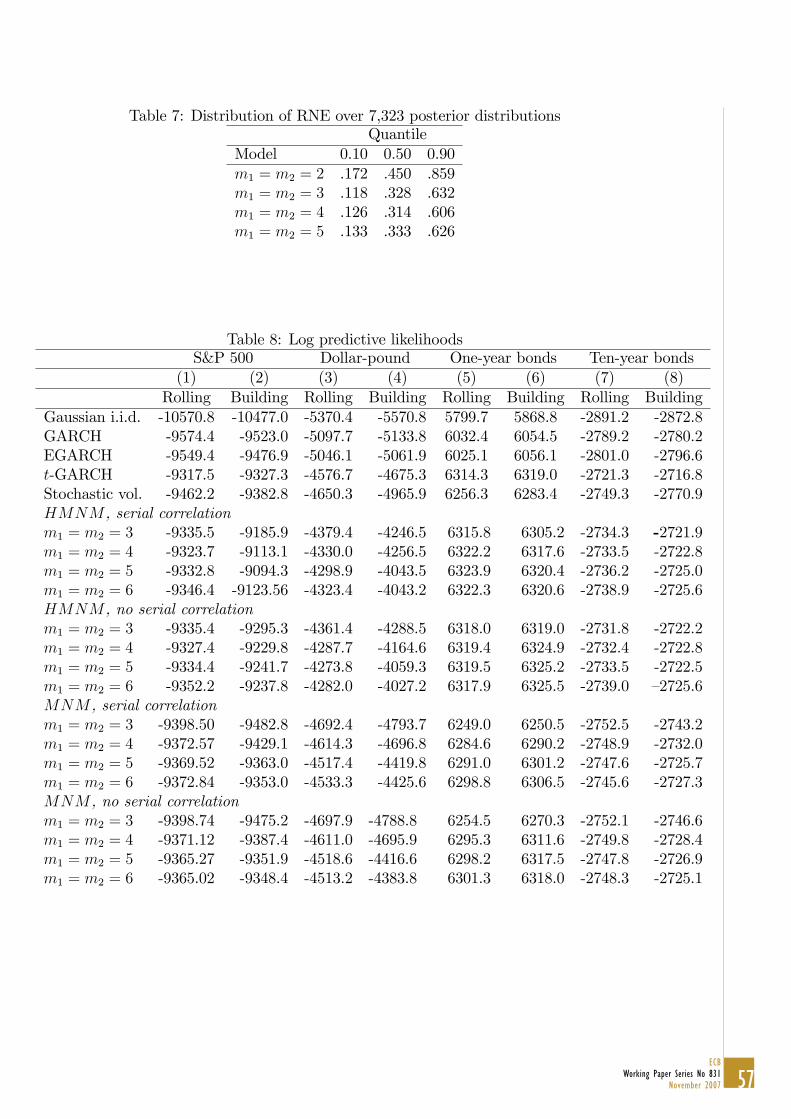
1) We compared our model with its main competitors (ARCH and Stochastic Volatility) using predictive likelihood ratios; we found out that for the bond data our model is on the same level as its competitors. For the stock returns and foreign exchange returns data sets, our model is respectively superior and overwhelmingly superior to the alternative models.

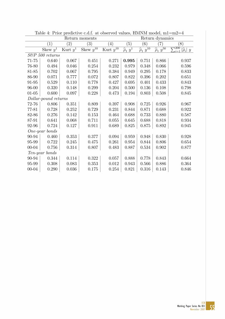
2) We examined the properties of the model generated conditional distributions. If the model is well specified, the cumulative density functions (CDFs) of these distributions, evaluated at realized returns, should be uniformly distributed and those for one-day horizons should be independent. The uniform distribution turns out to be an accurate description for one-day horizons, but deteriorates as the horizon lengthens. The one-day CDFs are positively autocorrelated.

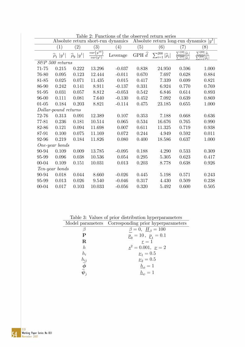
3) We examined whether the model’s posterior predictive distributions of the most important characteristics of asset returns are compatible with those observed in the data (posterior predictive distribution). For most characteristics, asset return series and time periods the answer is consistent with the observed characteristics. However, for the S&P 500 returns our model predicts much less serial correlation and smaller leverage effects than those observed, and it cannot account for the long-memory characteristics in the early 1970s.

Finally, we focus on periods of greatest volatility in the asset return series examined, showing how conditional distributions react to strong movements in returns, and studying how they readjust as the volatility returns to more usual values.


7ECB



9ECB



11ECB



13ECB



15ECB



17ECB



19ECB



21ECB



23ECB



25ECB



27ECB



29ECB



31ECB



33ECB



35ECB



37ECB



39ECB



41ECB



43ECB



45ECB



47ECB



49ECB



51ECB



53ECB



55ECB



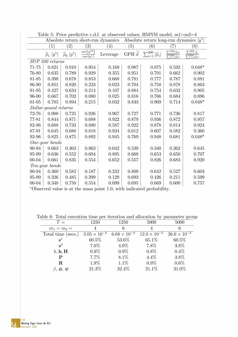
Table 5: Prior predictive c.d.f. at observed values, HMNM model, m1=m2=4Absolute return short-run dynamics Absolute return long-run dynamics jy1j(1) (2) (3) (4) (5) (6) (7) (8)b�1 jy1j b�9 jy1j var(y10)

var(y1)Leverage GPH bd P200

i=1 jb�ij P100i=1jb�ijP200i=1jb�ij

P200i=1 b�iP200i=1jb�ij

S&P 500 returns71-75 0.821 0.910 0.954 0.169 0.987 0.975 0.592 0.048*76-80 0.635 0.789 0.929 0.355 0.951 0.791 0.662 0.90281-85 0.398 0.678 0.853 0.668 0.781 0.777 0.787 0.88186-90 0.851 0.820 0.233 0.023 0.704 0.758 0.878 0.86391-95 0.427 0.634 0.214 0.107 0.884 0.754 0.632 0.90596-00 0.667 0.702 0.080 0.025 0.816 0.766 0.684 0.89601-05 0.785 0.894 0.215 0.032 0.833 0.969 0.714 0.048*Dollar-pound returns72-76 0.908 0.725 0.926 0.967 0.727 0.771 0.736 0.81777-81 0.844 0.871 0.688 0.922 0.879 0.936 0.872 0.95782-86 0.688 0.733 0.880 0.587 0.922 0.878 0.814 0.92487-91 0.645 0.688 0.818 0.934 0.612 0.607 0.582 0.36092-96 0.825 0.875 0.892 0.945 0.769 0.948 0.681 0.048*One-year bonds90-94 0.663 0.363 0.963 0.042 0.539 0.340 0.362 0.64595-99 0.636 0.552 0.694 0.895 0.668 0.653 0.650 0.70700-04 0.661 0.835 0.554 0.652 0.557 0.826 0.683 0.920Ten-year bonds90-94 0.360 0.582 0.187 0.232 0.809 0.642 0.527 0.60395-99 0.326 0.485 0.399 0.129 0.693 0.426 0.211 0.59900-04 0.348 0.750 0.554 0.099 0.695 0.669 0.600 0.757�Observed value is at the mass point 1.0, with indicated probability.

Table 6: Total execution time per iteration and allocation by parameter groupT = 1250 1250 5000 5000

m1 = m2 = 4 6 4 6Total time (secs.) 3:05� 10�3 6:68� 10�3 12:0� 10�3 26:6� 10�3

s1 60.5% 53.6% 65.1% 60.5%s2 7.6% 4.0% 7.8% 3.8%

h;h;H 0.9% 0.9% 0.8% 0.4%P 7.7% 8.1% 4.4% 3.8%R 1.9% 1.1% 0.9% 0.6%

�, �, 21.3% 32.4% 21.1% 31.0%

57ECB


Table 7: Distribution of RNE over 7,323 posterior distributionsQuantile

Model 0.10 0.50 0.90m1 = m2 = 2 .172 .450 .859m1 = m2 = 3 .118 .328 .632m1 = m2 = 4 .126 .314 .606m1 = m2 = 5 .133 .333 .626

Table 8: Log predictive likelihoodsS&P 500 Dollar-pound One-year bonds Ten-year bonds

(1) (2) (3) (4) (5) (6) (7) (8)Rolling Building Rolling Building Rolling Building Rolling Building

Gaussian i.i.d. -10570.8 -10477.0 -5370.4 -5570.8 5799.7 5868.8 -2891.2 -2872.8GARCH -9574.4 -9523.0 -5097.7 -5133.8 6032.4 6054.5 -2789.2 -2780.2EGARCH -9549.4 -9476.9 -5046.1 -5061.9 6025.1 6056.1 -2801.0 -2796.6t-GARCH -9317.5 -9327.3 -4576.7 -4675.3 6314.3 6319.0 -2721.3 -2716.8Stochastic vol. -9462.2 -9382.8 -4650.3 -4965.9 6256.3 6283.4 -2749.3 -2770.9HMNM , serial correlationm1 = m2 = 3 -9335.5 -9185.9 -4379.4 -4246.5 6315.8 6305.2 -2734.3 -2721.9m1 = m2 = 4 -9323.7 -9113.1 -4330.0 -4256.5 6322.2 6317.6 -2733.5 -2722.8m1 = m2 = 5 -9332.8 -9094.3 -4298.9 -4043.5 6323.9 6320.4 -2736.2 -2725.0m1 = m2 = 6 -9346.4 -9123.56 -4323.4 -4043.2 6322.3 6320.6 -2738.9 -2725.6HMNM , no serial correlationm1 = m2 = 3 -9335.4 -9295.3 -4361.4 -4288.5 6318.0 6319.0 -2731.8 -2722.2m1 = m2 = 4 -9327.4 -9229.8 -4287.7 -4164.6 6319.4 6324.9 -2732.4 -2722.8m1 = m2 = 5 -9334.4 -9241.7 -4273.8 -4059.3 6319.5 6325.2 -2733.5 -2722.5m1 = m2 = 6 -9352.2 -9237.8 -4282.0 -4027.2 6317.9 6325.5 -2739.0 �2725.6MNM , serial correlationm1 = m2 = 3 -9398.50 -9482.8 -4692.4 -4793.7 6249.0 6250.5 -2752.5 -2743.2m1 = m2 = 4 -9372.57 -9429.1 -4614.3 -4696.8 6284.6 6290.2 -2748.9 -2732.0m1 = m2 = 5 -9369.52 -9363.0 -4517.4 -4419.8 6291.0 6301.2 -2747.6 -2725.7m1 = m2 = 6 -9372.84 -9353.0 -4533.3 -4425.6 6298.8 6306.5 -2745.6 -2727.3MNM , no serial correlationm1 = m2 = 3 -9398.74 -9475.2 -4697.9 -4788.8 6254.5 6270.3 -2752.1 -2746.6m1 = m2 = 4 -9371.12 -9387.4 -4611.0 -4695.9 6295.3 6311.6 -2749.8 -2728.4m1 = m2 = 5 -9365.27 -9351.9 -4518.6 -4416.6 6298.2 6317.5 -2747.8 -2726.9m1 = m2 = 6 -9365.02 -9348.4 -4513.2 -4383.8 6301.3 6318.0 -2748.3 -2725.1


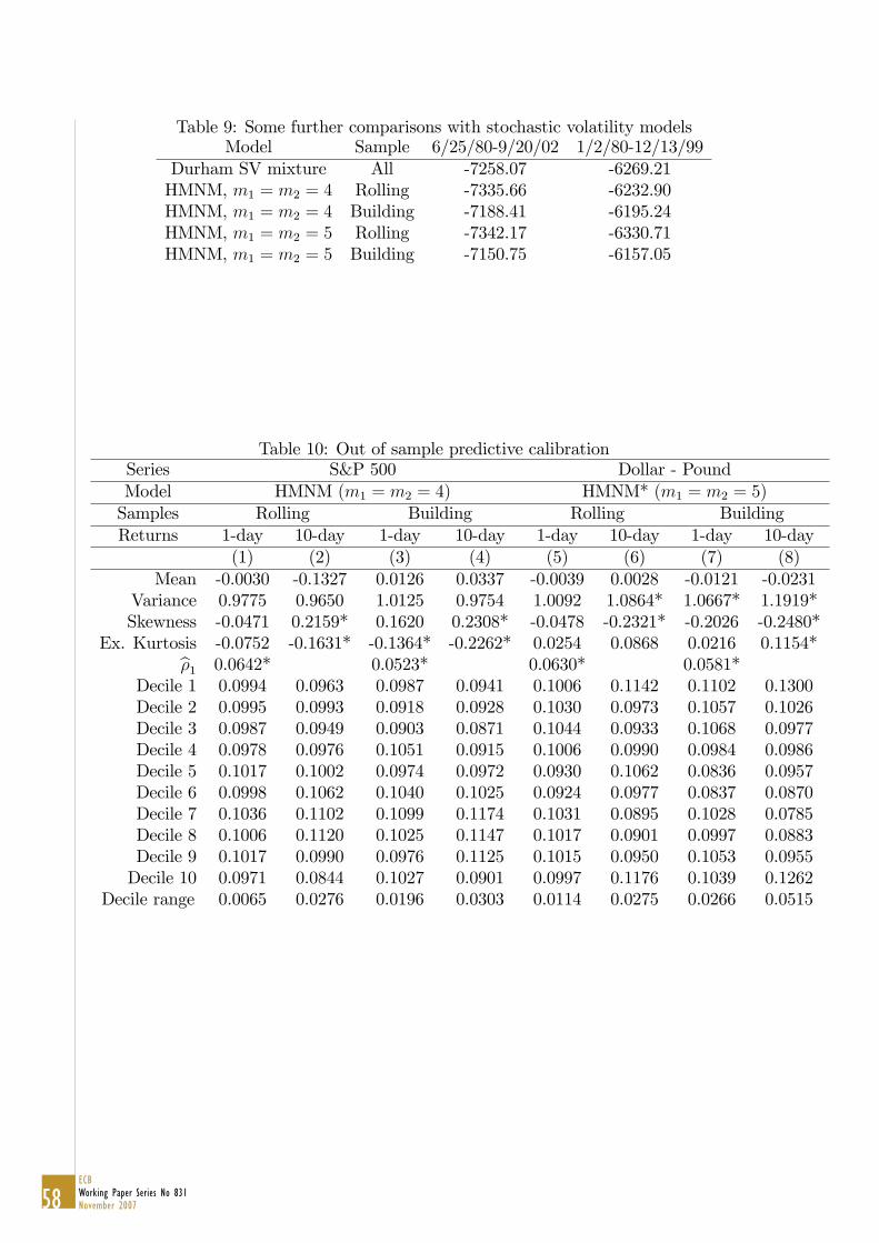
Table 9: Some further comparisons with stochastic volatility modelsModel Sample 6/25/80-9/20/02 1/2/80-12/13/99

Durham SV mixture All -7258.07 -6269.21HMNM, m1 = m2 = 4 Rolling -7335.66 -6232.90HMNM, m1 = m2 = 4 Building -7188.41 -6195.24HMNM, m1 = m2 = 5 Rolling -7342.17 -6330.71HMNM, m1 = m2 = 5 Building -7150.75 -6157.05

Table 10: Out of sample predictive calibrationSeries S&P 500 Dollar - PoundModel HMNM (m1 = m2 = 4) HMNM* (m1 = m2 = 5)Samples Rolling Building Rolling BuildingReturns 1-day 10-day 1-day 10-day 1-day 10-day 1-day 10-day

(1) (2) (3) (4) (5) (6) (7) (8)Mean -0.0030 -0.1327 0.0126 0.0337 -0.0039 0.0028 -0.0121 -0.0231

Variance 0.9775 0.9650 1.0125 0.9754 1.0092 1.0864* 1.0667* 1.1919*Skewness -0.0471 0.2159* 0.1620 0.2308* -0.0478 -0.2321* -0.2026 -0.2480*

Ex. Kurtosis -0.0752 -0.1631* -0.1364* -0.2262* 0.0254 0.0868 0.0216 0.1154*b�1 0.0642* 0.0523* 0.0630* 0.0581*Decile 1 0.0994 0.0963 0.0987 0.0941 0.1006 0.1142 0.1102 0.1300Decile 2 0.0995 0.0993 0.0918 0.0928 0.1030 0.0973 0.1057 0.1026Decile 3 0.0987 0.0949 0.0903 0.0871 0.1044 0.0933 0.1068 0.0977Decile 4 0.0978 0.0976 0.1051 0.0915 0.1006 0.0990 0.0984 0.0986Decile 5 0.1017 0.1002 0.0974 0.0972 0.0930 0.1062 0.0836 0.0957Decile 6 0.0998 0.1062 0.1040 0.1025 0.0924 0.0977 0.0837 0.0870Decile 7 0.1036 0.1102 0.1099 0.1174 0.1031 0.0895 0.1028 0.0785Decile 8 0.1006 0.1120 0.1025 0.1147 0.1017 0.0901 0.0997 0.0883Decile 9 0.1017 0.0990 0.0976 0.1125 0.1015 0.0950 0.1053 0.0955Decile 10 0.0971 0.0844 0.1027 0.0901 0.0997 0.1176 0.1039 0.1262

Decile range 0.0065 0.0276 0.0196 0.0303 0.0114 0.0275 0.0266 0.0515

59ECB


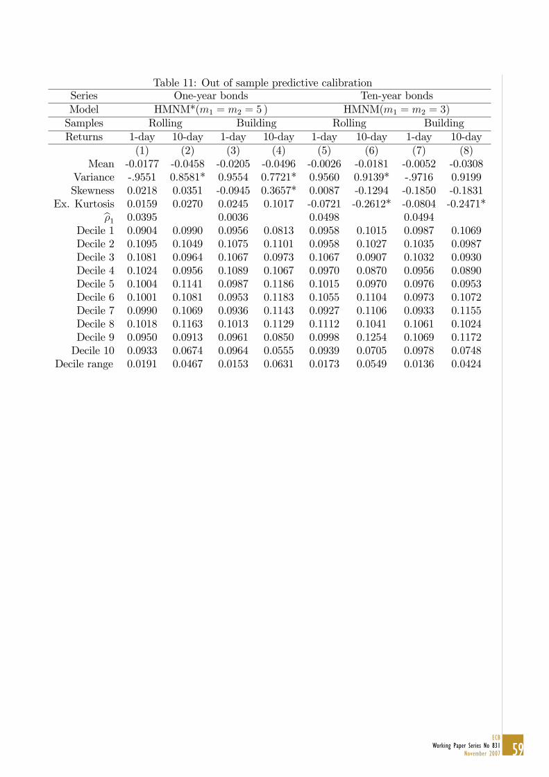
Table 11: Out of sample predictive calibrationSeries One-year bonds Ten-year bondsModel HMNM*(m1 = m2 = 5 ) HMNM(m1 = m2 = 3)Samples Rolling Building Rolling BuildingReturns 1-day 10-day 1-day 10-day 1-day 10-day 1-day 10-day

(1) (2) (3) (4) (5) (6) (7) (8)Mean -0.0177 -0.0458 -0.0205 -0.0496 -0.0026 -0.0181 -0.0052 -0.0308

Variance -.9551 0.8581* 0.9554 0.7721* 0.9560 0.9139* -.9716 0.9199Skewness 0.0218 0.0351 -0.0945 0.3657* 0.0087 -0.1294 -0.1850 -0.1831

Ex. Kurtosis 0.0159 0.0270 0.0245 0.1017 -0.0721 -0.2612* -0.0804 -0.2471*b�1 0.0395 0.0036 0.0498 0.0494Decile 1 0.0904 0.0990 0.0956 0.0813 0.0958 0.1015 0.0987 0.1069Decile 2 0.1095 0.1049 0.1075 0.1101 0.0958 0.1027 0.1035 0.0987Decile 3 0.1081 0.0964 0.1067 0.0973 0.1067 0.0907 0.1032 0.0930Decile 4 0.1024 0.0956 0.1089 0.1067 0.0970 0.0870 0.0956 0.0890Decile 5 0.1004 0.1141 0.0987 0.1186 0.1015 0.0970 0.0976 0.0953Decile 6 0.1001 0.1081 0.0953 0.1183 0.1055 0.1104 0.0973 0.1072Decile 7 0.0990 0.1069 0.0936 0.1143 0.0927 0.1106 0.0933 0.1155Decile 8 0.1018 0.1163 0.1013 0.1129 0.1112 0.1041 0.1061 0.1024Decile 9 0.0950 0.0913 0.0961 0.0850 0.0998 0.1254 0.1069 0.1172Decile 10 0.0933 0.0674 0.0964 0.0555 0.0939 0.0705 0.0978 0.0748

Decile range 0.0191 0.0467 0.0153 0.0631 0.0173 0.0549 0.0136 0.0424


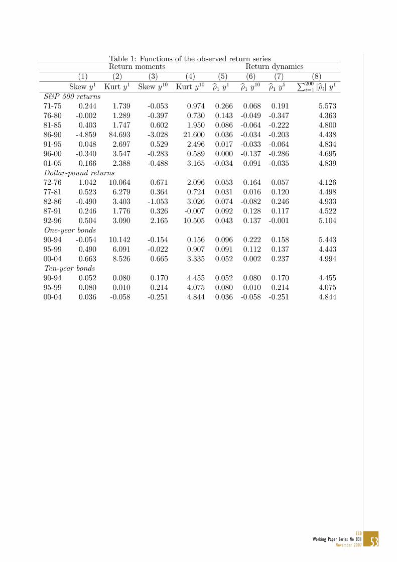
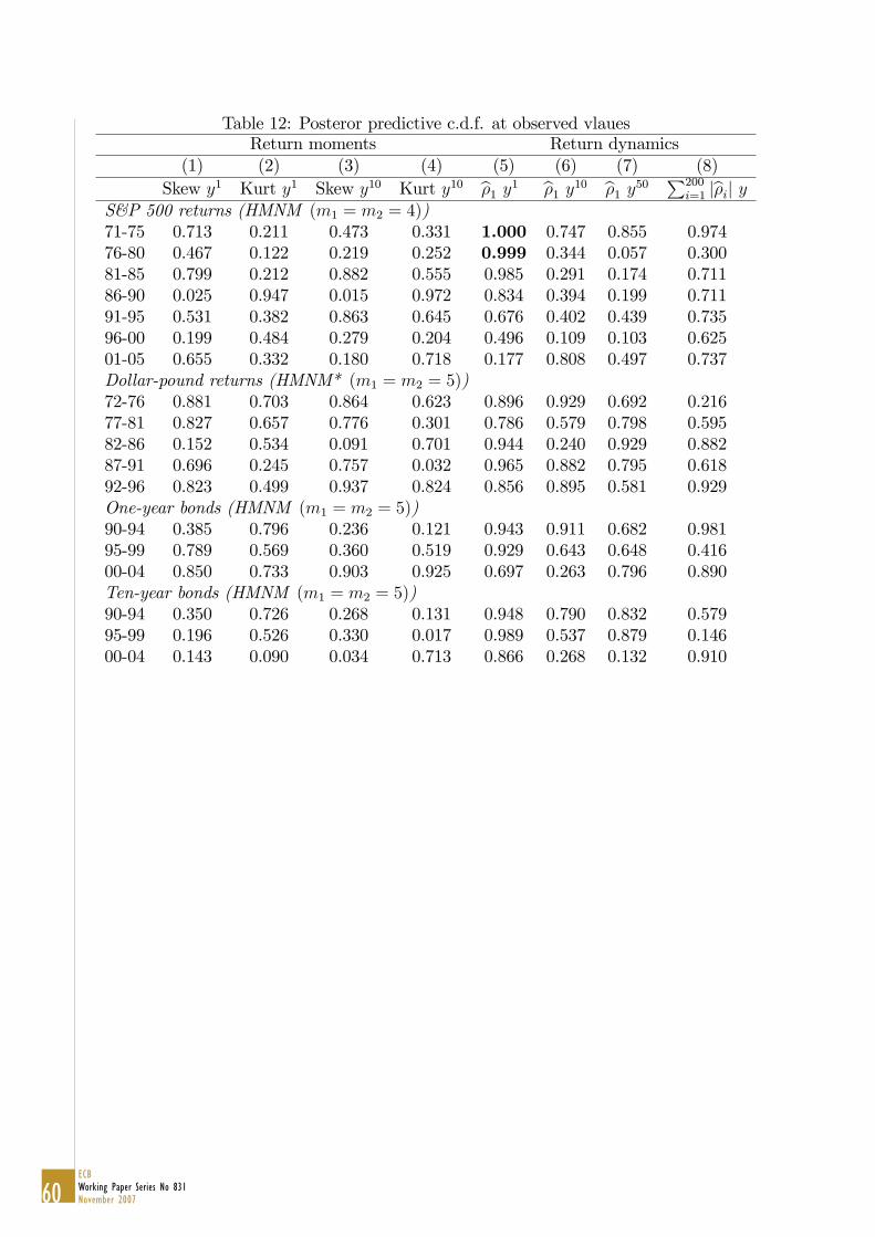
Table 12: Posteror predictive c.d.f. at observed vlauesReturn moments Return dynamics

(1) (2) (3) (4) (5) (6) (7) (8)Skew y1 Kurt y1 Skew y10 Kurt y10 b�1 y1 b�1 y10 b�1 y50 P200

i=1 jb�ij yS&P 500 returns (HMNM (m1 = m2 = 4))71-75 0.713 0.211 0.473 0.331 1.000 0.747 0.855 0.97476-80 0.467 0.122 0.219 0.252 0.999 0.344 0.057 0.30081-85 0.799 0.212 0.882 0.555 0.985 0.291 0.174 0.71186-90 0.025 0.947 0.015 0.972 0.834 0.394 0.199 0.71191-95 0.531 0.382 0.863 0.645 0.676 0.402 0.439 0.73596-00 0.199 0.484 0.279 0.204 0.496 0.109 0.103 0.62501-05 0.655 0.332 0.180 0.718 0.177 0.808 0.497 0.737Dollar-pound returns (HMNM* (m1 = m2 = 5))72-76 0.881 0.703 0.864 0.623 0.896 0.929 0.692 0.21677-81 0.827 0.657 0.776 0.301 0.786 0.579 0.798 0.59582-86 0.152 0.534 0.091 0.701 0.944 0.240 0.929 0.88287-91 0.696 0.245 0.757 0.032 0.965 0.882 0.795 0.61892-96 0.823 0.499 0.937 0.824 0.856 0.895 0.581 0.929One-year bonds (HMNM (m1 = m2 = 5))90-94 0.385 0.796 0.236 0.121 0.943 0.911 0.682 0.98195-99 0.789 0.569 0.360 0.519 0.929 0.643 0.648 0.41600-04 0.850 0.733 0.903 0.925 0.697 0.263 0.796 0.890Ten-year bonds (HMNM (m1 = m2 = 5))90-94 0.350 0.726 0.268 0.131 0.948 0.790 0.832 0.57995-99 0.196 0.526 0.330 0.017 0.989 0.537 0.879 0.14600-04 0.143 0.090 0.034 0.713 0.866 0.268 0.132 0.910

61ECB


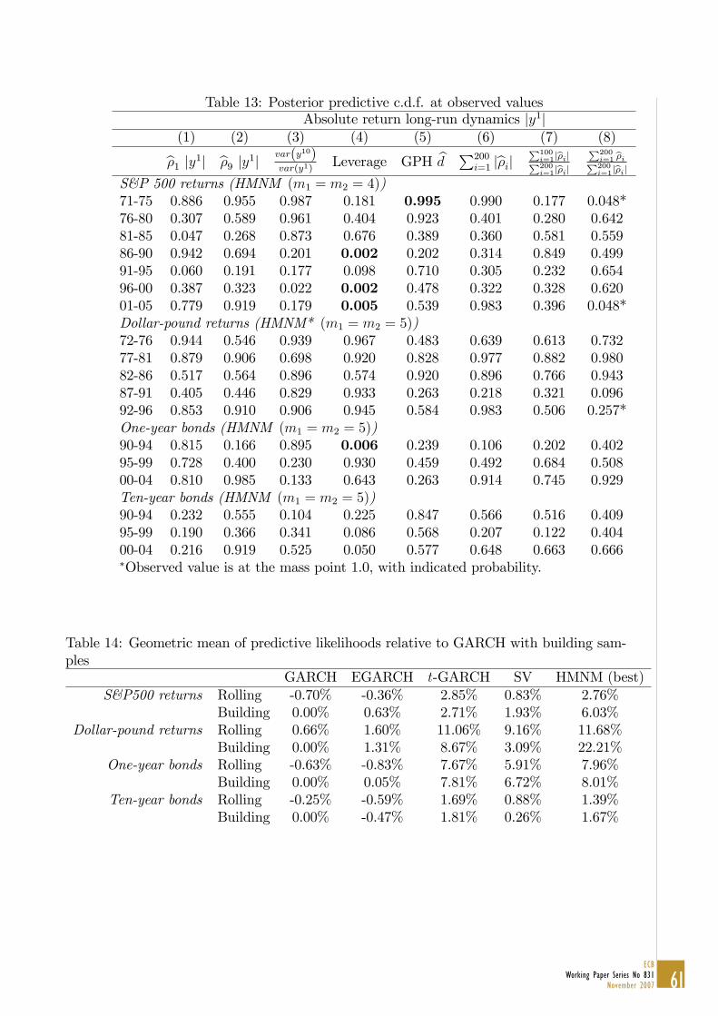
Table 13: Posterior predictive c.d.f. at observed valuesAbsolute return long-run dynamics jy1j

(1) (2) (3) (4) (5) (6) (7) (8)b�1 jy1j b�9 jy1j var(y10)var(y1)

Leverage GPH bd P200i=1 jb�ij P100

i=1jb�ijP200i=1jb�ij

P200i=1 b�iP200i=1jb�ij

S&P 500 returns (HMNM (m1 = m2 = 4))71-75 0.886 0.955 0.987 0.181 0.995 0.990 0.177 0.048*76-80 0.307 0.589 0.961 0.404 0.923 0.401 0.280 0.64281-85 0.047 0.268 0.873 0.676 0.389 0.360 0.581 0.55986-90 0.942 0.694 0.201 0.002 0.202 0.314 0.849 0.49991-95 0.060 0.191 0.177 0.098 0.710 0.305 0.232 0.65496-00 0.387 0.323 0.022 0.002 0.478 0.322 0.328 0.62001-05 0.779 0.919 0.179 0.005 0.539 0.983 0.396 0.048*Dollar-pound returns (HMNM* (m1 = m2 = 5))72-76 0.944 0.546 0.939 0.967 0.483 0.639 0.613 0.73277-81 0.879 0.906 0.698 0.920 0.828 0.977 0.882 0.98082-86 0.517 0.564 0.896 0.574 0.920 0.896 0.766 0.94387-91 0.405 0.446 0.829 0.933 0.263 0.218 0.321 0.09692-96 0.853 0.910 0.906 0.945 0.584 0.983 0.506 0.257*One-year bonds (HMNM (m1 = m2 = 5))90-94 0.815 0.166 0.895 0.006 0.239 0.106 0.202 0.40295-99 0.728 0.400 0.230 0.930 0.459 0.492 0.684 0.50800-04 0.810 0.985 0.133 0.643 0.263 0.914 0.745 0.929Ten-year bonds (HMNM (m1 = m2 = 5))90-94 0.232 0.555 0.104 0.225 0.847 0.566 0.516 0.40995-99 0.190 0.366 0.341 0.086 0.568 0.207 0.122 0.40400-04 0.216 0.919 0.525 0.050 0.577 0.648 0.663 0.666�Observed value is at the mass point 1.0, with indicated probability.

Table 14: Geometric mean of predictive likelihoods relative to GARCH with building sam-ples

GARCH EGARCH t-GARCH SV HMNM (best)S&P500 returns Rolling -0.70% -0.36% 2.85% 0.83% 2.76%

Building 0.00% 0.63% 2.71% 1.93% 6.03%Dollar-pound returns Rolling 0.66% 1.60% 11.06% 9.16% 11.68%

Building 0.00% 1.31% 8.67% 3.09% 22.21%One-year bonds Rolling -0.63% -0.83% 7.67% 5.91% 7.96%

Building 0.00% 0.05% 7.81% 6.72% 8.01%Ten-year bonds Rolling -0.25% -0.59% 1.69% 0.88% 1.39%

Building 0.00% -0.47% 1.81% 0.26% 1.67%


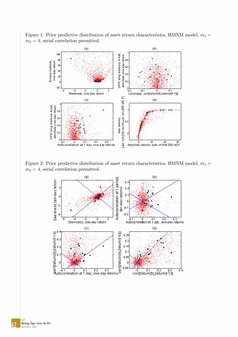
Figure 1: Prior predictive distribution of asset return characteristics, HMNM model, m1 =m2 = 4, serial correlation permitted.

Figure 2: Prior predictive distribution of asset return characteristics, HMNM model, m1 =m2 = 4, serial correlation permitted.

63ECB


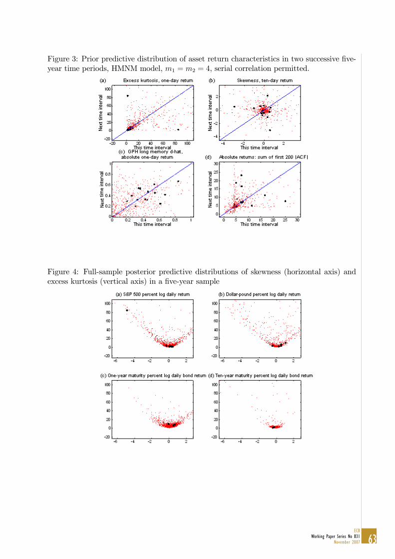
Figure 3: Prior predictive distribution of asset return characteristics in two successive �ve-year time periods, HMNM model, m1 = m2 = 4, serial correlation permitted.

Figure 4: Full-sample posterior predictive distributions of skewness (horizontal axis) andexcess kurtosis (vertical axis) in a �ve-year sample


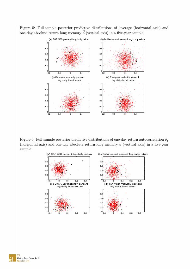
Figure 5: Full-sample posterior predictive distributions of leverage (horizontal axis) andone-day absolute return long memory bd (vertical axis) in a �ve-year sample

Figure 6: Full-sample posterior predictive distributions of one-day return autocorrelation b�1(horizontal axis) and one-day absolute return long memory bd (vertical axis) in a �ve-yearsample

65ECB


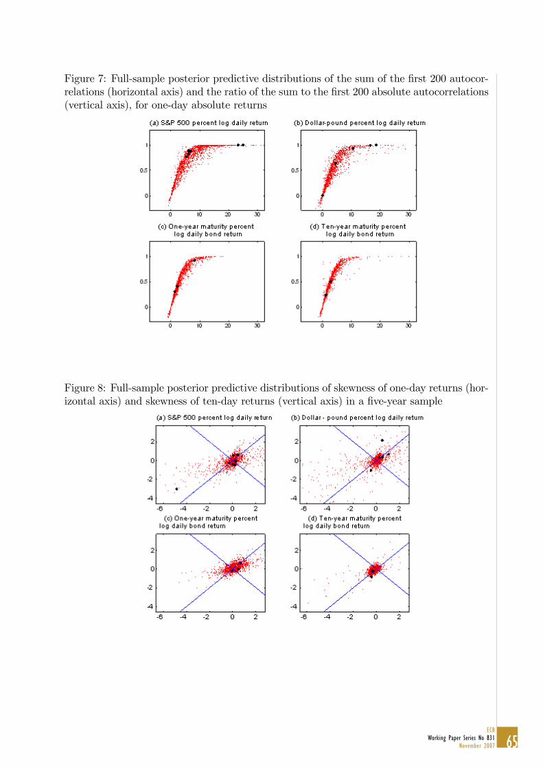
Figure 7: Full-sample posterior predictive distributions of the sum of the �rst 200 autocor-relations (horizontal axis) and the ratio of the sum to the �rst 200 absolute autocorrelations(vertical axis), for one-day absolute returns

Figure 8: Full-sample posterior predictive distributions of skewness of one-day returns (hor-izontal axis) and skewness of ten-day returns (vertical axis) in a �ve-year sample


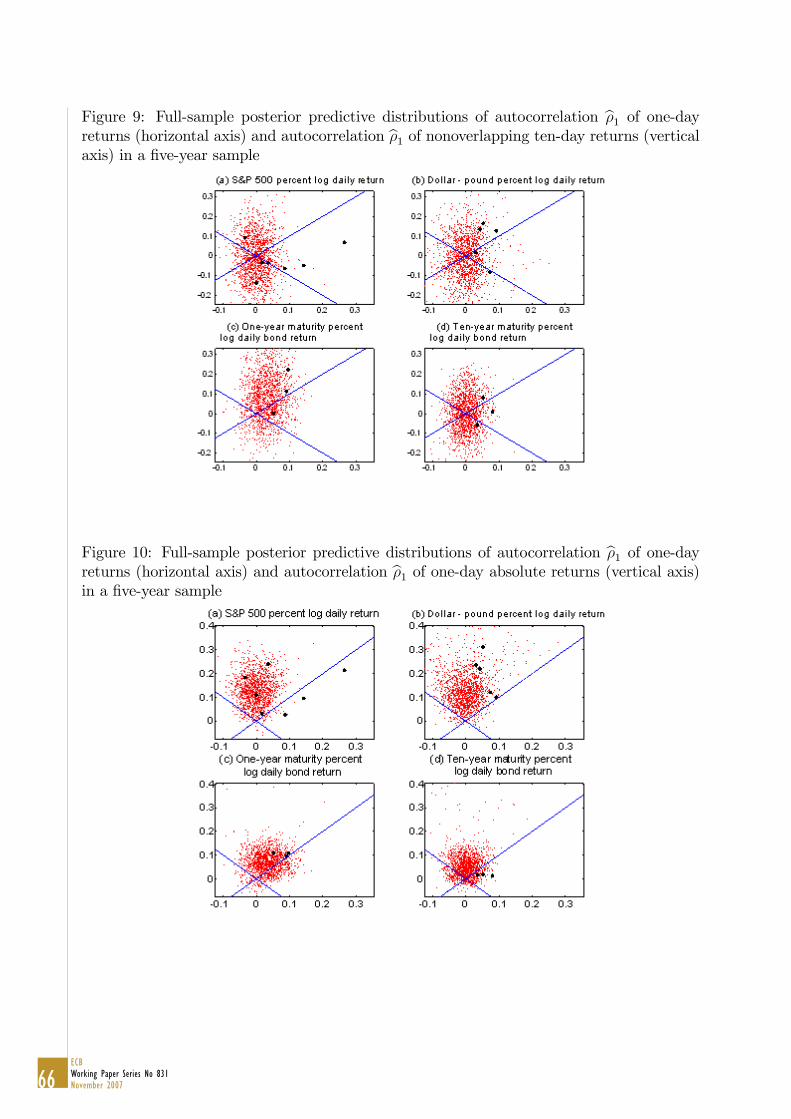
Figure 9: Full-sample posterior predictive distributions of autocorrelation b�1 of one-dayreturns (horizontal axis) and autocorrelation b�1 of nonoverlapping ten-day returns (verticalaxis) in a �ve-year sample

Figure 10: Full-sample posterior predictive distributions of autocorrelation b�1 of one-dayreturns (horizontal axis) and autocorrelation b�1 of one-day absolute returns (vertical axis)in a �ve-year sample

67ECB


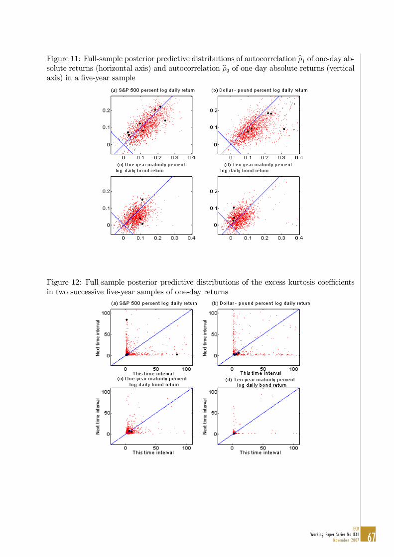
Figure 11: Full-sample posterior predictive distributions of autocorrelation b�1 of one-day ab-solute returns (horizontal axis) and autocorrelation b�9 of one-day absolute returns (verticalaxis) in a �ve-year sample

Figure 12: Full-sample posterior predictive distributions of the excess kurtosis coe¢ cientsin two successive �ve-year samples of one-day returns


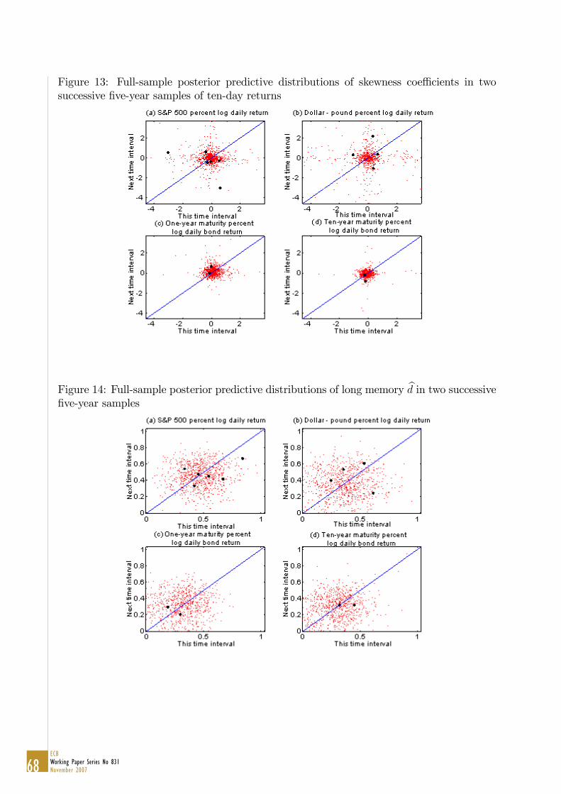
Figure 13: Full-sample posterior predictive distributions of skewness coe¢ cients in twosuccessive �ve-year samples of ten-day returns

Figure 14: Full-sample posterior predictive distributions of long memory bd in two successive�ve-year samples

69ECB


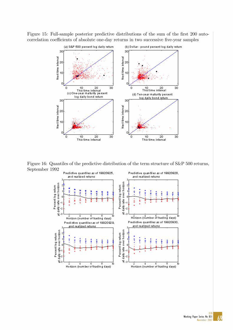
Figure 15: Full-sample posterior predictive distributions of the sum of the �rst 200 auto-correlation coe¢ cients of absolute one-day returns in two successive �ve-year samples

Figure 16: Quantiles of the predictive distribution of the term structure of S&P 500 returns,September 1992


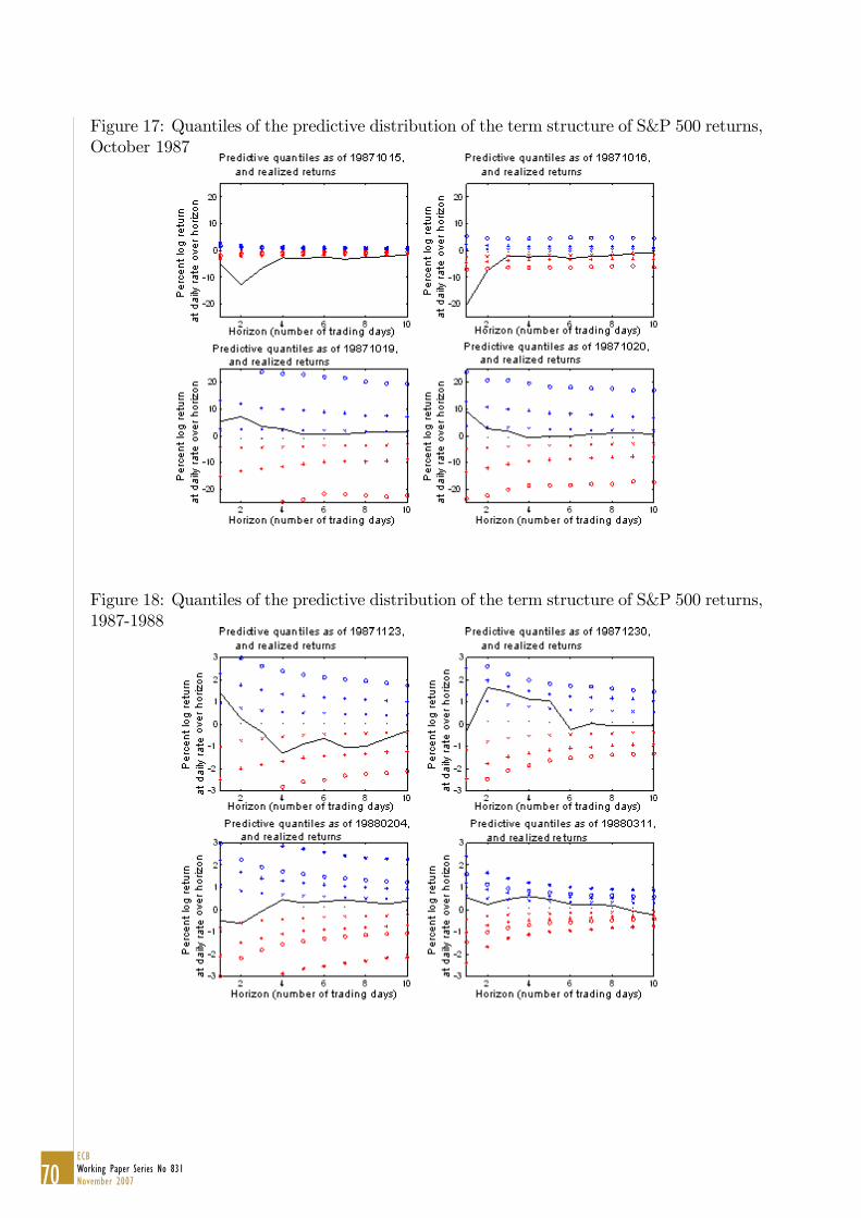
Figure 17: Quantiles of the predictive distribution of the term structure of S&P 500 returns,October 1987

Figure 18: Quantiles of the predictive distribution of the term structure of S&P 500 returns,1987-1988

71ECB


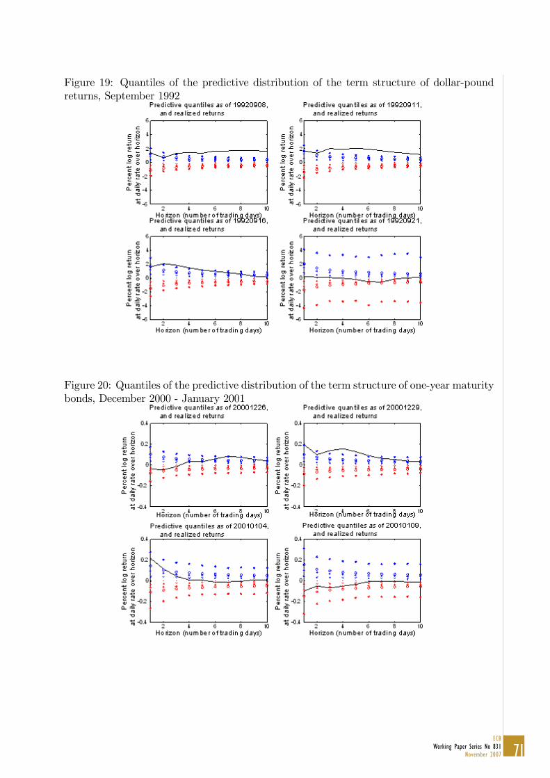
Figure 19: Quantiles of the predictive distribution of the term structure of dollar-poundreturns, September 1992

Figure 20: Quantiles of the predictive distribution of the term structure of one-year maturitybonds, December 2000 - January 2001


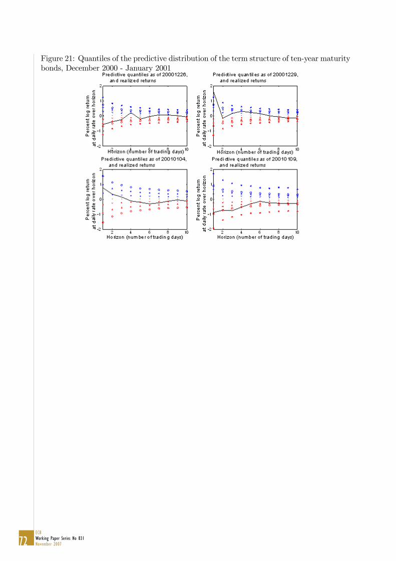
Figure 21: Quantiles of the predictive distribution of the term structure of ten-year maturitybonds, December 2000 - January 2001

73ECB


European Central Bank Working Paper Series

For a complete list of Working Papers published by the ECB, please visit the ECB’s website (http://www.ecb.europa.eu).

790 “Asset prices, exchange rates and the current account” by M. Fratzscher, L. Juvenal and L. Sarno, August 2007.

791 “Inquiries on dynamics of transition economy convergence in a two-country model” by J. Brůha and

J. Podpiera, August 2007.

792 “Euro area market reactions to the monetary developments press release” by J. Coffi net and S. Gouteron,

August 2007.

793 “Structural econometric approach to bidding in the main refi nancing operations of the Eurosystem”

by N. Cassola, C. Ewerhart and C. Morana, August 2007.

794 “(Un)naturally low? Sequential Monte Carlo tracking of the US natural interest rate” by M. J. Lombardi and

S. Sgherri, August 2007.

795 “Assessing the impact of a change in the composition of public spending: a DSGE approach” by R. Straub and

I. Tchakarov, August 2007.

796 “The impact of exchange rate shocks on sectoral activity and prices in the euro area” by E. Hahn, August 2007.

797 “Joint estimation of the natural rate of interest, the natural rate of unemployment, expected infl ation, and

potential output” by L. Benati and G. Vitale, August 2007.

798 “The transmission of US cyclical developments to the rest of the world” by S. Dées and I. Vansteenkiste,

August 2007.

799 “Monetary policy shocks in a two-sector open economy: an empirical study” by R. Llaudes, August 2007.

800 “Is the corporate bond market forward looking?” by J. Hilscher, August 2007.

801 “Uncovered interest parity at distant horizons: evidence on emerging economies & nonlinearities” by A. Mehl

and L. Cappiello, August 2007.

802 “Investigating time-variation in the marginal predictive power of the yield spread” by L. Benati and

C. Goodhart, August 2007.

803 “Optimal monetary policy in an estimated DSGE for the euro area” by S. Adjemian, M. Darracq Pariès and

S. Moyen, August 2007.

804 “Growth accounting for the euro area: a structural approach” by T. Proietti and A. Musso, August 2007.

805 “The pricing of risk in European credit and corporate bond markets” by A. Berndt and I. Obreja, August 2007.

806 “State-dependency and fi rm-level optimization: a contribution to Calvo price staggering” by P. McAdam and

A. Willman, August 2007.

807 “Cross-border lending contagion in multinational banks” by A. Derviz and J. Podpiera, September 2007.

808 “Model misspecifi cation, the equilibrium natural interest rate and the equity premium” by O. Tristani,

September 2007.

809 “Is the New Keynesian Phillips curve fl at?” by K. Kuester, G. J. Müller and S. Stölting, September 2007.


810 “Infl ation persistence: euro area and new EU Member States” by M. Franta, B. Saxa and K. Šmídková,

September 2007.

811 “Instability and nonlinearity in the euro area Phillips curve” by A. Musso, L. Stracca and D. van Dijk,

September 2007.

812 “The uncovered return parity condition” by L. Cappiello and R. A. De Santis, September 2007.

813 “The role of the exchange rate for adjustment in boom and bust episodes” by R. Martin, L. Schuknecht and

I. Vansteenkiste, September 2007.

814 “Choice of currency in bond issuance and the international role of currencies” by N. Siegfried, E. Simeonova

and C. Vespro, September 2007.

815 “Do international portfolio investors follow fi rms’ foreign investment decisions?” by R. A. De Santis and

P. Ehling, September 2007.

816 “The role of credit aggregates and asset prices in the transmission mechanism: a comparison between the euro

area and the US” by S. Kaufmann and M. T. Valderrama, September 2007.

817 “Convergence and anchoring of yield curves in the euro area” by M. Ehrmann, M. Fratzscher, R. S. Gürkaynak

and E. T. Swanson, October 2007.

818 “Is time ripe for price level path stability?” by V. Gaspar, F. Smets and D. Vestin, October 2007.

819 “Proximity and linkages among coalition participants: a new voting power measure applied to the International

Monetary Fund” by J. Reynaud, C. Thimann and L. Gatarek, October 2007.

820 “What do we really know about fi scal sustainability in the EU? A panel data diagnostic” by A. Afonso and

C. Rault, October 2007.

821 “Social value of public information: testing the limits to transparency” by M. Ehrmann and M. Fratzscher,

October 2007.

822 “Exchange rate pass-through to trade prices: the role of non-linearities and asymmetries” by M. Bussière,

October 2007.

823 “Modelling Ireland’s exchange rates: from EMS to EMU” by D. Bond and M. J. Harrison and E. J. O’Brien,

October 2007.

824 “Evolving U.S. monetary policy and the decline of infl ation predictability” by L. Benati and P. Surico,

October 2007.

825 “What can probability forecasts tell us about infl ation risks?” by J. A. García and A. Manzanares,

October 2007.

826 “Risk sharing, fi nance and institutions in international portfolios” by M. Fratzscher and J. Imbs, October 2007.

827 “How is real convergence driving nominal convergence in the new EU Member States?”

by S. M. Lein-Rupprecht, M. A. León-Ledesma and C. Nerlich, November 2007.

828 “Potential output growth in several industrialised countries: a comparison” by C. Cahn and A. Saint-Guilhem,

November 2007.

829 “Modelling infl ation in China: a regional perspective” by A Mehrotra, T. Peltonen and A. Santos Rivera,

November 2007.

75ECB


830 “The term structure of euro area break-even infl ation rates: the impact of seasonality” by J. Ejsing, J. A. García

and T. Werner, November 2007.

831 “Hierarchical Markov normal mixture models with applications to fi nancial asset returns”

by J. Geweke and G. Amisano, November 2007.

Date: 15 Nov, 2007 14:42:29;Format: (420.00 x 297.00 mm);Output Profile: SPOT IC300;Preflight: Failed!

Date post:	08-Apr-2018
Category:	Documents
Upload:	buihanh
View:	215 times
Download:	0 times

Hierarchical Markov normal mixture models with ... · working paper series no 831 / november 2007...

Documents