Hierarchical O(N) Computation of Small-Angle

Scattering Profiles and their Associated Derivatives

Konstantin Berlin∗, Nail A. Gumerov†, David Fushman‡, and Ramani Duraiswami§

University of Maryland, College Park

May 07, 2012

Abstract

Fast algorithms for Debye summation, which arises in computations performed in crystal-

lography, small/wide-angle X-ray scattering (SAXS/WAXS) and small-angle neutron scatter-

ing (SANS), were recently presented in Gumerov et al. (J. Comput. Chem., 2012, 33, 1981).

∗Equal first author, Department of Chemistry and Biochemistry, Center for Biomolecular Structure and Orga-

nization, and Institute for Advanced Computer Studies; all at the University of Maryland, College Park, MD;

email:kberlin@umd.edu web:https://sites.google.com/site/kberlin/†Equal first author, Institute for Advanced Computer Studies, University of Maryland, College Park, MD; and at

Fantalgo, LLC, Elkridge, MD; email: gumerov@umiacs.umd.edu; web:http://www.umiacs.umd.edu/

users/gumerov‡Department of Chemistry and Biochemistry, Center for Biomolecular Structure and Organization, and Institute

for Advanced Computer Studies, all at University of Maryland, College Park, MD; email:fushman@umd.edu;

web:http://www.chem.umd.edu/research/facultyprofiles/davidfushman§Department of Computer Science and Institute for Advanced Computer Studies, University of Maryland, College

Park, MD; and at Fantalgo, LLC; email: ramani@umiacs.umd.edu; web:http://www.umiacs.umd.edu/

users/ramani

1

The use of these algorithms can speed up computation of scattering profiles in macromolecular

structure refinement protocols. However, these protocols often employ an iterative gradient-

based optimization procedure, which then requires derivatives of the profile with respect to

atomic coordinates. An extension to one of the algorithms is presented which allows accurate,

O(N) cost computation of the derivatives along with the scattering profile. Computational

results show orders of magnitude improvement in computational efficiency, while maintaining

prescribed accuracy. This opens the possibility to efficiently integrate small-angle scattering

data into structure determination and refinement of macromolecular systems.

Keywords: Small Angle Scattering (SAS), Wide Angle Scattering (WAS), Jacobian, Gradient

10−1 10010−5

10−4

10−3

10−2

q ( A -1)

I(q)

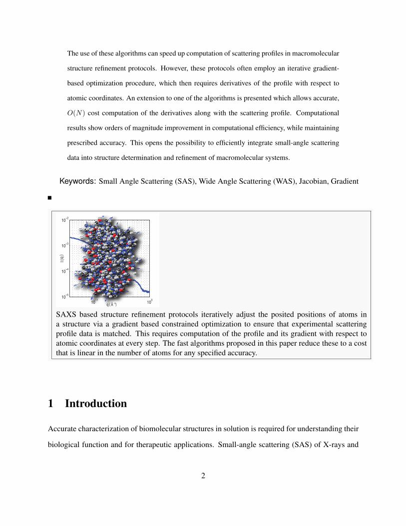
SAXS based structure refinement protocols iteratively adjust the posited positions of atoms ina structure via a gradient based constrained optimization to ensure that experimental scatteringprofile data is matched. This requires computation of the profile and its gradient with respect toatomic coordinates at every step. The fast algorithms proposed in this paper reduce these to a costthat is linear in the number of atoms for any specified accuracy.

1 Introduction

Accurate characterization of biomolecular structures in solution is required for understanding their

biological function and for therapeutic applications. Small-angle scattering (SAS) of X-rays and

2

neutrons can indirectly measure the distribution of interatomic distances of a molecule in solu-

tion, providing a set of structural restraints [1]. As a result, solution SAS studies have become

increasingly used in structural biology, with a broad range of applications including structure re-

finement of biological macromolecules and their complexes [2, 3, 4, 5], analysis of conformational

ensembles and flexibility in solution [6, 7, 8, 9], and high-throughput structural studies [10, 11].

In order to use SAS experimental data as an atomic-level structural restraint, the SAS pro-

file needs to be predicted ab initio from the assumed molecular atomic structure, which requires

computing all-pairs interactions of the atoms in the molecule (also referred to as an N -body prob-

lem). In addition, this computation must be performed numerous times in an iterative structure

refinement algorithm [2, 12] or for a high-throughput structural analysis.

Several approximation methods have been proposed to speed up this computation [13, 14, 12,

15]. However, depending on the size of the molecule, the approximations can introduce significant

errors [16]. Recently we developed and demonstrated a hierarchical harmonic expansion method,

based on the fast multipole method (FMM), which has superior asymptotical performance than pre-

viously proposed approximation methods, while maintaining any prescribed accuracy [16]. This

large speedup in computation has the potential to significantly improve integration of SAS into

structure refinement protocols, like Xplor-NIH [17] and HADDOCK [18], where the scattering

profile needs to be computed thousands of times during iterative structure refinement.

A potential problem with integrating SAS data into a structure refinement protocol is the need

to accurately and quickly compute the gradient (“force”) of the SAS profile, in addition to the

actual SAS profile [19]. In order to save on computation time it was suggested in [20] to ap-

proximate the low-frequency part of the SAS profile using Taylor expansion. The drawback of

this approach is that significant structural information contained in the higher-frequency region of

the scattering profile is ignored. Furthermore, the low-frequency profile region becomes smaller

as the molecule size increases, since this approximation depends on the magnitude of the prod-

uct of the wavenumber and molecule size. An alternative approach was suggested in [3], where

3

the gradient was approximated by taking the derivative of the scattering amplitude explicitly, and

then averaged over a large number of orientations. However, since no error guarantees are given,

this approximation might result in an incorrect gradient direction, significantly slowing down any

derivative-based structure optimization method. In addition to the computational complexity of the

derivative computation, macromolecules can be combined with a solvation layer, to improve the

accuracy of the SAS profile prediction [12]. These additional water molecules, especially the large

number of atoms that result from discretizing a continuous water model, can significantly increase

the computation time needed for estimation of the SAS profile and its derivatives [21, 15, 22].

Here we propose an extension to the method proposed in [16] to achieve an accurate and fast

method for the simultaneous computation of the full scattering profile and associated gradients.

The method completely avoids computationally intractable all-to-all atom summations. We show

that it is possible to quickly and accurately compute the gradient of the SAS profile using the al-

gorithm developed here so that the computation only slightly adds to the overall computation time

compared to just a straight computation of the profile in [16]. Furthermore, leveraging the compu-

tational advantages of the hierarchical approach, we demonstrate that the profile and derivatives for

a macromolecule solvated in a very dense water grid can be computed many orders of magnitude

faster than by current methods.

2 Method

The SAS profile value of an N atom system such as a macromolecule and associated solvent

molecules can be computed as

I(ri, . . . , rN ; q) =⟨|A (q)|2

⟩Ω, (1)

4

for q = q1 . . . qQ, where

A (q) =N∑j=1

fj (q) exp (iq · rj) (2)

is the scattering amplitude from the particle in vacuo, q = |q| is the scattering wavenumber (q =

(4π/λ) sinϑ, 2ϑ is the scattering angle, λ the wavelength), rj = [xj, yj, zj] is the position of the

jth atom, fj(q) is the form factor of the jth atom, and 〈·〉Ω indicates averaging of q over a sphere,

to reflect averaging over all possible molecular orientations in solution or powder.

Equation (1) can be analytically averaged, such that

⟨|A (q)|2

⟩Ω

=N∑i=1

fi(q)N∑j=1

fj(q)s(qrij) =N∑i=1

fi(q)Ψi, (3)

where s is the sinc function,

s(qrij) =sin(q‖ri − rj‖2)

q‖ri − rj‖2

, (4)

Ψi is defied as in Eq. 3, and ‖·‖2 is the Euclidean norm.

In order to refine macromolecule structure, uniquely defined by its atomic positions [ri, . . . , rN ],

against experimentally collected scattering data, the discrepancy between the experimental scatter-

ing, Iexp(q) and the predicted scattering, I(ri, . . . , rN ; q), for q = q1 . . . qQ, is minimized. To

resolve the structural degeneracy of SAS, additional energy terms coming from NMR, X-ray crys-

tallography, other structural methods, and force fields restraints may also be used. This refinement

is typically formulated as an energy minimization problem,

minri,...,rN

χ2(ri, . . . , rN) + Λ(ri, . . . , rN), (5)

where

χ2(ri, . . . , rN) =

Q∑k=1

‖I(ri, . . . , rN ; qk)− Iexp(qk)‖22 = ‖d‖2

2 =

Q∑k=1

d2k, (6)

is the discrepancy of between the predicted and the experimental scattering profile, and Λ(ri, . . . , rN)

5

is the weight of all the other structural restraints, as well as potential regularization terms. In the

sequel we abbreviate I(ri, . . . , rN ; qk) as Ik.

The cost of computing the profile I in Eq. ((1)) requires the sums in Eq. ((3)), which has

O(N2) computational cost, if done directly. A widely used computer program, CRYSOL [13],

uses truncated harmonic expansions to speed up the computations. In [16] it was shown that

without an associated error bound, the harmonic expansion methods are likely to give incorrect

results, especially at large q. Two fast algorithms, based on hierarchical decomposition of the

spatial domain, local spherical expansion and translation, were presented in the paper. One of these

algorithms, is used in this paper to develop an extended algorithm, which can for a slight increase

in cost, compute the derivatives of the profile with respect to the Cartesian atomic coordinates.

2.1 Computation of Derivatives

We focus on ε-accurate computation of the gradient of I(q), sometimes referred to as the “force”

of I(q), which is required for a local convex optimization of Eq. (5) using a Newton-type mini-

mization, such as done in Xplore-NIH (as well as other programs). Computation of the Hessian

is typically avoided, either by an iterative approximations of the Hessian using a quasi-Newton

method, or in the case of least-squares, an approximation based on the Jacobian [23].

Assuming the derivatives of Λ are already computed, based on the linearity of differentiation,

in order to compute the gradient of Eq. (5) we only need to compute the Jacobian of I(q),

J =

∂I1∂x1

∂I1∂y1

∂I1∂z1

. . . ∂I1∂xN

∂I1∂yN

∂I1∂zN

. . . . . . . . . . . . . . . . . . . . . . . . . . . . . . . . . .

∂IQ∂x1

∂IQ∂y1

∂IQ∂z1

. . .∂IQ∂xN

∂IQ∂yN

∂IQ∂zN

, (7)

where J is a Q× 3N matrix. From the Jacobian, the gradient can be computed as

∇χ2 = 2JTd, (8)

6

and the Hessian can be approximated as

H ≈ 2JJT + 2λI, (9)

where I is the identity matrix, for some λ ∈ [0, 1], in the case of a least-squares method. In case of

an iterative quasi-Newton minimization of equation Eq. (5), only equation Eq. (8) is needed, and

the Hessian is iteratively updated.

Without loss of generality for ∂Ik∂yi

and ∂Ik∂zi

,

∂Ik∂xi

= 2fi(qk)Ψ′i = 2fi(qk)N∑j=1

fj(qk)s′(qkrij), (10)

where s′(qkrnj) and Ψ′i are the partial derivatives with respect to xi. The derivative s′(qkrnj) can

be analytically computed as

s′(qkrij) = (xi − xj)[

cos(qkrij)

r2ij

− sin(qkrij)

qkr3ij

], (11)

for rij 6= 0. Therefore, direct computation of J (and∇χ2) has complexity of O(N2Q).

The N2 computational complexity can be avoided if we first expand Ψi using an expansion in

terms of spherical basis functions Rmn (r) as

Ψi =m=n∑m=−n

Rmn (ri)B

mn (rj) + εp, (12)

and

Bmn (rj) = 4π

N∑j=1

fj(q)R−mn (rj) (13)

7

for all i, where Rmn is a regular spherical basis function

Rmn (r) = jn(qr)Y m

n (s) = jn(qr)Y mn (θ, ϕ) , r = rs. (14)

FunctionsRmn (r) here are given in spherical coordinates (r, θ, ϕ), r =r (sin θ cosϕ, sin θ sinϕ, cos θ),

where jn(qr) are spherical Bessel functions, while Y mn (θ, ϕ) are the normalized spherical harmon-

ics of degree n and order m,

Y mn (θ, ϕ) = (−1)m

√2n+ 1

4π

(n− |m|)!(n+ |m|)!

P |m|n (cos θ)eimϕ, (15)

n = 0, 1, 2, ...; m = −n, ..., n.

where P |m|n (µ) are the associated Legendre functions consistent with that in [24], or Rodrigues’

formulae

Pmn (µ) = (−1)m

(1− µ2

)m/2 dm

dµmPn (µ) , n > 0, m > 0, (16)

Pn (µ) =1

2nn!

dn

dµn

(µ2 − 1

)n, n > 0,

where Pn (µ) are the Legendre polynomials.

Here p and εp are the cutoff degree and associated error respectively. This expansion can be

quickly computed for Ψi, for all i = 1, . . . , N , using the hierarchical algorithm in O(p3 log(p) +

N logN) time [16]. However, unlike the basic case of straight computation of I(q), a downward

pass is now required because individualRmn (ri) values also need to be computed for the derivatives.

Once Eq. (12) is computed, taking the derivative of Eq. (12) yields

Ψ′i =

p−1∑n=0

m=n∑m=−n

R′mn (ri)B

mn (rj) + εp, (17)

8

where the derivative of the spherical function, R′mn , has been derived in [26], and is given in the

Supplementary Information section. This derivative can be written as a weighted linear combina-

tion of two to four adjacent spherical basis functions (depending on the particular spatial derivative

needed), where the weights are independent of ri, and accordingly can be expressed as the product

of a sparse matrix with the expansion coefficients. Therefore,

Ψ′i =

p−1∑n=0

m=n∑m=−n

Rmn (ri)α

m(j)n + εp, (18)

where αm(j)n can be quickly computed by a sparse O(p2) matrix multiplication, and is the same

for all Ψ′i. As noted in the original reference, the error bound for derivative computations require

slightly higher truncation numbers, which are one or two higher than those for the expansion of Ψ.

Thus the overall complexity of computing J, given that the harmonic expansion has already

been computed for all Ψi for all q, is O(p2NQ). The proper value of p for a specific value of q

is proportional to qD, where D is the diameter of the molecule (largest distance between any two

atoms) [16]. Therefore, the overall complexity of the gradient computation is O(Q3D2N), for an

arbitrary error bound.

3 Results

The computational complexity of the hierarchical algorithm is dependent on the atomic density of

the molecule. This complexity also extends to the computation of the Jacobian, since since it is

directly dependent on speed of the spherical expansion of I(q). To specifically quantify the advan-

tages of our approach for biological macromolecules, we compare the computational speed of our

algorithm to direct all-to-all computation of eqs. (3,10) (“Direct”), vs. spherical harmonic expan-

sion method like CRYSOL [13], the properly error truncated version, “Middleman” [16], and the

hierarchical method (“Hierarchical,” which combines the above expressions for the derivative with

9

the algorithm in [16]) for various sized random and actual macromolecules, solvated at different

water layer densities.

3.1 Derivatives

We ran the benchmarks on a Dual Quad-Core Intel Xeon X5560 CPU @ 2.80GHz 64bit Linux ma-

chine with 24GB ECC DDR3 SDRAM. All programs were compiled using the Intel 11.1 compiler

using the “-parallel -O3 -ipo” flags. We timed the computational time for generating a SAS profile

made out of 50 uniformly spaced evaluations of the profile on the range 0.01 ≤ q ≤ 0.5 A−1, for

a randomly generated molecule with atomic density of d = 0.02 A−3

. The timing and accuracy

results for the randomly generated molecules are presented in Fig. 1.

103 104 105 10610−2

10−1

100

101

102

103

N

Tim

e(s

)

DirectMiddlemanHierarchical

103 104 10510−10

10−8

10−6

10−4

10−2

N

Rela

tive

Err

or

10−3

10−6

10−9

(A) (B)

Figure 1: Results for randomly generated proteins, timing for uniformly distributed 50 pointscattering profile, 0 < q ≤ 0.5 A

−1. (A) Computation time for just the SAS profile (dashed), and

the SAS profile with Jacobian (solid). (B) Maximum relative error in the Jacobian, as measured bymaxi‖Ji,∗ − Ji,∗‖2/‖Ji,∗‖2, where J is the true Jacobian, and Ji,∗ is the ith row of J.

Fig. 1A shows that computation of the derivatives does not change the asymptotic properties of

any of the algorithms. For the hierarchical method, the computation of the Jacobian increases the

computation time by about 3.5. This increase is partially because of the addition of a downward

10

pass in our hierarchical method. The hierarchical method, with or without Jacobian computation,

is faster than the CRYSOL-like “Middleman” algorithm, as well as direct computation. Fig. 1B

shows that the accuracy of the Jacobian computation is within an order of magnitude of the pre-

scribed accuracy for I(q).

3.2 Water Layer

We have demonstrated the computational improvement of our algorithm, compared to the direct

and middleman algorithm, at approximate atomic density of proteins. However, one of the princi-

pal advantages of our hierarchical method is that we decouple the number of atoms from molecule’s

diameter in the computation. This gives us a large computational advantage over previous ap-

proaches when computing SAS profile of dense objects. We now show that for macromolecules

solvated in a dense water grid layer, such that the overall atomic density increases without signifi-

cantly increasing the molecule’s diameter, the speedup of our hierarchical algorithm becomes even

larger.

We choose two proteins, archaeal peroxiredoxin (PDB 2E2G) and diubiquitin (PDB 1AAR),

that have very different atomic density (distribution of inter-atomic distances) to illustrate the

speedup the algorithm provides. Archaeal peroxiredoxin has a large empty cavity in the center

(see Fig. 2). The number of atoms for PDB 1AAR increases from 2575 atoms, with no water layer,

to several orders of magnitude larger 548462 atoms for 0.5 A water layer grid. For PDB 2E2G

the number of atoms increases from 39609, to 543832 atoms for a slightly coarser minimum 1.0 A

water layer grid. Good speedup of our algorithm compared to previously published algorithms can

be seen in Fig. 3.

Fig. 3 demonstrates that not only is our hierarchical approach significantly faster, the speedup

gets progressively larger at higher water density.

11

Figure 2: Cartoon representation of (A) PDB 1AAR, (B) PDB 2E2G.

0.5124810−1

100

101

102

103

Wate r Grid Density (A )

Tim

e(s

)

DirectMiddlemanHierarchical

1248100

101

102

103

Wate r Grid Density (A )

Tim

e(s

)

DirectMiddlemanHierarchical

(A) (B)

Figure 3: Timing results for computation of the profile (just SAS profile is dashed line, and SASprofile with the Jacobian is solid line), with an 8 A water layer, at different water grid densities(inter-atomic distances). (A) PDB 1AAR, (B) PDB 2E2G.

4 Discussion

The computational advantage of the algorithm presented for large and dense molecules can be

understood in terms of how it relates to the three main alternatives for computing I(q): (i) direct

all-to-all summation of Eq. (3); (ii) numerical integration or averaging of Eq. (1), as suggested in

12

[2, 14, 15]; and (iii) analytical expansion of Eq. (2) [13, 27]. As discussed in [16], approach (i)

has O(N2) complexity, making it intractable for larger macromolecules, while (ii,iii) approaches

are bounded by the bandwidth of Eq. (2), requiring either O(q2D2) function evaluations or basis

functions in order to accurately approximate the scattering profile, resulting in O(q2D2N) compu-

tational complexity. Additionally, a spherical harmonic series expansion of A (q) is not sparse, so

it is not possible to accurately approximate Eq. (3) using non-uniform sampling of the sphere.

When considering large and/or dense molecules, whereD orN is large, all the three approaches

become computationally intractable. However, a large speedup is possible if we compute an ap-

proximate series expansion of Eq. (2) faster than in O(q2D2N) time. That is the main idea behind

our hierarchical method, where only a small expansion is performed locally, where D is small,

and then translated hierarchically onto progressively larger domains. This grouping of adjacent

atoms together is somewhat similar to the intuitive idea of grouping of atoms by their secondary

structure as suggested in [27]. However, because grouping is done at multiple hierarchical levels

and combined together using proven theoretical bounds, this paradigm allows much faster com-

putation, can be made arbitrarily accurate, and can better accommodate various macromolecular

shapes (including cavities).

As the result of the hierarchical grouping of atoms, our algorithm has O((qD)3 log(qD) +

N logN) complexity for each I(q) evaluation, which is a significant theoretical improvement for

large molecules and dense water models, because it separates the size of the domain, D, from the

number of atoms in the macromolecule, N . In practice, this allows us to accurately compute I(q)

for extremely large systems made of millions of atoms or even when the water density is high

enough to well approximate a continuous water model. As a byproduct of this computation, we

also compute the O(q2D2)-sized series expansion of Eq. (3). Once this expansion is computed,

the derivatives of the minimization function can be quickly computed by taking the derivative of

each basis function.

Even though the hierarchical method is faster than direct spherical harmonic expansions of

13

I(q), it is not required for computing the Jacobian, since only the final series expansion is needed

to compute the derivative. This implies that programs like CRYSOL, which are based on direct

series expansion of Eq. (2), can be easily adapted to compute derivatives using Eq. (18), as long

as the series expansion is properly truncated according to a proper error bound.

The hierarchical approach is not limited to strict spatial subdivision of macromolecules, and

can be adapted to use various other groupings, including secondary structures, or other rigid com-

ponents, further speeding up the computation. For certain applications the derivatives for the water

molecules might be required. Our hierarchical approach allows us to take advantage of this case by

computing a downward pass only on the required atomic domain, if necessary. We note that this

algorithm is a proof of principle, and thus the performance can be significantly improved, either

by improving the translation operators or by removing complex number multiplications in several

instances.

5 Conclusion

We developed and demonstrated a fast method for computation of SAS profile, and its associ-

ated derivatives with respect to atomic coordinates of the molecule. The method is based on our

previously developed hierarchical expansion method, and is able to compute the SAS profile and

associated derivatives to within arbitrary ε accuracy, while being an order of magnitude faster than

current method. The algorithm’s computational advantage is even larger for high density atom

distribution, which can occur when discretizing continuous water models. This opens up the pos-

sibility to efficiently integrate small-angle scattering data into the existing protocols for structure

determination and refinement of macromolecular systems.

14

6 Acknowledgments

This study has been partially supported by the New Research Frontiers Award of the Institute of

the Advanced Computer Studies of the University of Maryland, by Fantalgo, LLC., and by NIH

grant GM065334 to D.F.

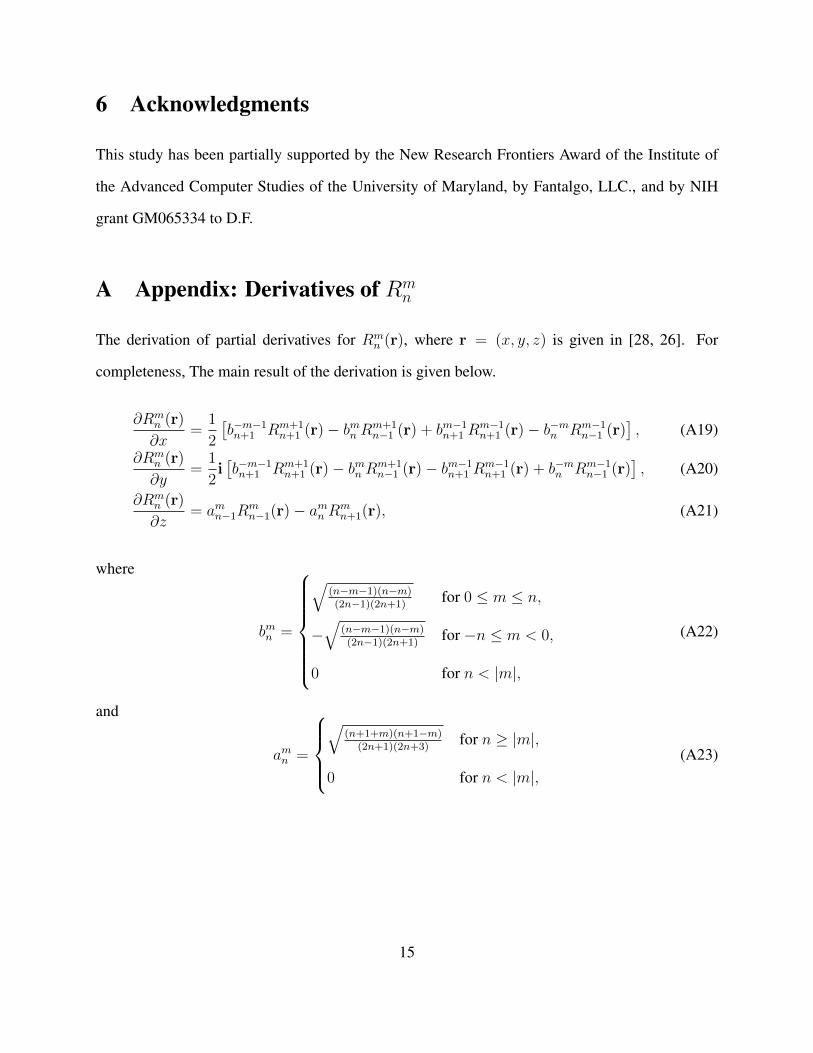
A Appendix: Derivatives of Rmn

The derivation of partial derivatives for Rmn (r), where r = (x, y, z) is given in [28, 26]. For

completeness, The main result of the derivation is given below.

∂Rmn (r)

∂x=

1

2

[b−m−1n+1 Rm+1

n+1 (r)− bmn Rm+1n−1 (r) + bm−1

n+1 Rm−1n+1 (r)− b−mn Rm−1

n−1 (r)], (A19)

∂Rmn (r)

∂y=

1

2i[b−m−1n+1 Rm+1

n+1 (r)− bmn Rm+1n−1 (r)− bm−1

n+1 Rm−1n+1 (r) + b−mn Rm−1

n−1 (r)], (A20)

∂Rmn (r)

∂z= amn−1R

mn−1(r)− amn Rm

n+1(r), (A21)

where

bmn =

√(n−m−1)(n−m)(2n−1)(2n+1)

for 0 ≤ m ≤ n,

−√

(n−m−1)(n−m)(2n−1)(2n+1)

for −n ≤ m < 0,

0 for n < |m|,

(A22)

and

amn =

√

(n+1+m)(n+1−m)(2n+1)(2n+3)

for n ≥ |m|,

0 for n < |m|,(A23)

15

References

1. Koch, M. H. J.; Vachette, P. and Svergun, D. I., Quarterly Reviews of Biophysics, 2003, 36(02),

147–227.

2. Grishaev, A.; Tugarinov, V.; Kay, L. E.; Trewhella, J. and Bax, A., Journal of Biomolecular

NMR, 2008, 40(2), 95–106.

3. Grishaev, A.; Ying, J.; Canny, M.; Pardi, A. and Bax, A., Journal of Biomolecular NMR, 2008,

42(2), 99–109.

4. Grishaev, A.; Wu, J.; Trewhella, J. and Bax, A., Journal of the American Chemical Society,

2005, 127(47), 16621–16628.

5. Pons, C.; D’Abramo, M.; Svergun, D. I.; Orozco, M.; Bernado, P. and Fernandez-Recio, J.,

Journal of Molecular Biology, 2010, 403(2), 217–230.

6. Bernado, P.; Modig, K.; Grela, P.; Svergun, D. I.; Tchorzewski, M.; Pons, M. and Akke, M.,

Biophysical Journal, 2010, 98(10), 2374–2382.

7. Datta, A.; Hura, G. and Wolberger, C., Journal of Molecular Biology, 2009, 392(5), 1117–

1124.

8. Jehle, S.; Vollmar, B. S.; Bardiaux, B.; Dove, K. K.; Rajagopal, P.; Gonen, T.; Oschkinat, H.

and Klevit, R. E., Proceedings of the National Academy of Sciences, 2011.

9. Bernado, P.; Mylonas, E.; Petoukhov, M. V.; Blackledge, M. and Svergun, D. I., Journal of the

American Chemical Society, 2007, 129(17), 5656–5664.

10. Hura, G. L.; Menon, A. L.; Hammel, M.; Rambo, R. P.; Poole Ii, F. L.; Tsutakawa, S. E.;

Jenney Jr, F. E.; Classen, S.; Frankel, K. A.; Hopkins, R. C. and others, , Nature Methods,

2009, 6(8), 606–612.

16

11. Grant, T. D.; Luft, J. R.; Wolfley, J. R.; Tsuruta, H.; Martel, A.; Montelione, G. T. and Snell,

E. H., Biopolymers, 2011, 95(8).

12. Grishaev, A.; Guo, L.; Irving, T. and Bax, A., Journal of the American Chemical Society,

2010, 132(44), 15484–15486.

13. Svergun, D. I.; Barberato, C. and Koch, M. H. J., Journal of Applied Crystallography, 1995,

28(6), 768–773.

14. Bardhan, J.; Park, S. and Makowski, L., Journal of Applied Crystallography, 2009, 42(5),

932–943.

15. Poitevin, F.; Orland, H.; Doniach, S.; Koehl, P. and Delarue, M., Nucleic Acids Research,

2011, 39(suppl 2), W184–W189.

16. Gumerov, N. A.; Berlin, K.; Fushman, D. and Duraiswami, R., Journal of Computational

Chemistry, 2012, 33(25), 1981–1996.

17. Schwieters, C. D.; Kuszewski, J. J.; Tjandra, N. and Marius Clore, G., Journal of Magnetic

Resonance, 2003, 160(1), 65–73.

18. Dominguez, C.; Boelens, R. and Bonvin, A., NMR-based docking of protein-protein com-

plexes, 2003, 125, 51.

19. Brunger, A. T.; Adams, P. D.; Clore, G. M.; DeLano, W. L.; Gros, P.; Grosse-Kunstleve, R. W.;

Jiang, J.-S.; Kuszewski, J.; Nilges, M.; Pannu, N. S. and others, , Acta Crystallographica

Section D: Biological Crystallography, 1998, 54(5), 905–921.

20. Gabel, F.; Simon, B. and Sattler, M., European Biophysics Journal, 2006, 35(4), 313–327.

21. Stumpe, M. C.; Blinov, N.; Wishart, D.; Kovalenko, A. and Pande, V. S., The Journal of

Physical Chemistry B, 2010, 115(2), 319–328.

17

22. Virtanen, J. J.; Makowski, L.; Sosnick, T. R. and Freed, K. F., Biophysical journal, 2011,

101(8), 2061–2069.

23. Boyd, S. and Vandenberghe, L., Convex Optimization, Cambridge university press, 2004.

24. Abramowitz, M. and Stegun, I. A., National Bureau of Standsards, Applied Mathematics Se-

ries, 1970, 55.

25. Gumerov, N. A.; Berlin, K.; Fushman, D. and Duraiswami, R. A hierarchical algorithm for

fast Debye summation with applications to small angle scattering Technical report, University

of Maryland, 2011.

26. Gumerov, N. A. and Duraiswami, R., Fast Multipole Methods For the Helmholtz Equation in

Three Dimensions, Elsevier Science, 2004.

27. Liu, H.; Morris, R. J.; Hexemer, A.; Grandison, S. and Zwart, P. H., Acta Crystallographica

Section A: Foundations of Crystallography, 2012, 68(2), 0–0.

28. Gumerov, N. A. and Duraiswami, R., SIAM Journal on Scientific Computing, 2004, 25(4),

1344–1381.

18