Digital Object Identifier (DOI) 10.1007/s00220-013-1878-8Commun. Math. Phys. 326, 287–327 (2014) Communications in
MathematicalPhysics
Higgs Bundles and UV Completion in F-Theory
Ron Donagi1, Martijn Wijnholt2
1 Department of Mathematics, University of Pennsylvania, Philadelphia, PA 19104-6395, USA2 Max Planck Institute (Albert Einstein Institute), Am Mühlenberg 1, 14476 Potsdam-Golm, Germany.
Abstract: F-theory admits 7-branes with exceptional gauge symmetries, which canbe compactified to give phenomenological four-dimensional GUT models. Here westudy general supersymmetric compactifications of eight-dimensional Yang–Mills the-ory. They are mathematically described by meromorphic Higgs bundles, and thereforeadmit a spectral cover description. This allows us to give a rigorous and intrinsic con-struction of local models in F-theory. We use our results to prove a no-go theoremshowing that local SU (5) models with three generations do not exist for generic mod-uli. However we show that three-generation models do exist on the Noether–Lefschetzlocus. We explain how F-theory models can be mapped to non-perturbative orientifoldmodels using a scaling limit proposed by Sen. Further we address the construction ofglobal models that do not have heterotic duals, considering models with base CP3 or ablow-up thereof as examples. We show how one may obtain a contractible worldvolumewith a two-cycle not inherited from the bulk, a necessary condition for implementingGUT breaking using fluxes.
Recently [1–3] initiated a systematic effort to study a new class of Kaluza–Klein modelsfor Grand Unification. The basic idea was to use an eight-dimensional gauge theory withan exceptional gauge group, coupled to ten-dimensional type IIb supergravity. Althoughthis theory is non-renormalizable, there is a lot of evidence that it admits a UV completionwhich is called F-theory [4]. For practical purposes however, very little is known aboutthis non-perturbative completion, as it is not in reach of perturbative string theory. Weessentially only know the low energy gauge theory and supergravity Lagrangians, whichare uniquely determined by the symmetries. To get a weakly coupled description in whichthese Lagrangians can be trusted, the fields must be slowly varying. Thus these modelscan still have a weakly coupled description if we take a large volume limit. Recent workon F-theory models includes [5–20].
A central role in the analysis is played by local models, by which we mean Calabi–Yau fourfolds consisting of an ALE fibration over a compact complex surface S, orsometimes a minimal compactification thereof. Despite the conceptual progress in[1–3], there were a number of unanswered questions about the explicit constructionof local models in F-theory. In particular, the strategy in [1] (and also [3]) relied ontaking a limiting form of models with a heterotic dual. This approach yields manifestlyconsistent models, but it was perhaps less than clear if the most general local F-theorymodel is recovered this way. The approach in [2] is to postulate the matter curves andthe fluxes restricted to the matter curves. At first sight this looks more flexible, but inthis case it is less clear if the data is mutually consistent. Given the uncertainties, it canbe hard to evaluate what F-theory does or does not predict.
The first purpose of this paper is to give a rigorous and intrinsic construction of localF-theory models. The chain of logic is as follows. As mentioned above, the basic idea isthat in order to get a weakly coupled description, we want to construct compactificationsof a supersymmetric eight-dimensional gauge theory. We show that such compactifica-tions are mathematically described by meromorphic Higgs bundles on S. Unfortunatelysuch Higgs bundles are practically impossible to write down explicitly, and furthermorethey look very different from the traditional description of F-theory, which uses ellipti-cally fibered fourfolds. To address this, we are going to discuss explicit isomorphismsbetween the (holomorphic data of the) following three types of objects:
Higgs bundles ←→ spectral covers ←→ ALE fibrations. (1.1)
The first arrow is a relatively well-known fact about Higgs bundles. (Its relevance toF-theory was noted independently in [10], which appeared while this project was writtenup.) The second arrow however has not been appreciated, and it is the one that allowsus to make contact with the older descriptions of F-theory. The existence of these
Higgs Bundles and UV Completion in F-Theory 289
equivalences, explained in Sect. 2.4, is one of our key messages in the first part of thispaper.
Now the first and the third object in (1.1) are not so suitable for constructions. Inthe case of Higgs bundles, although this description is weakly coupled in the derivativeexpansion, the problem is that the hermitian metric on the bundle satisfies a non-linearPDE and is practically impossible to write explicitly. For ALE fibrations, the problem isthat a crucial part of the data is given by the G-flux (or more precisely a relative Delignecohomology class). The spectral cover approach is the most transparent, thus it is thisapproach that allows us to make constructions, particularly of the fluxes, and computethe spectrum and interactions.
Finally, our ALE fibrations should admit an elliptic fibration as well. If we assume thiselliptic fibration to be generically non-degenerate, then this singles out the ALE spacescorresponding to the exceptional groups.1 These are also exactly the ALE fibrationsthat one obtains from a scaling limit of heterotic/F-theory duality. Thus, the modelsobtained from our original strategy are actually rather general, in particular they do notrequire heterotic duals. We will discuss in Sect. 2.1 how an E8 structure emerges whenwe extract a local model from a global model, in agreement with the argument above.Furthermore, it is clear that our logic is not limited to F-theory. A completely parallelconstruction of local M-theory models based on a set of equivalences analogous to (1.1)will appear in [22].
The spectral cover approach allows us to give a precise description of the configurationspace of local F-theory models, which is important for phenomenological applications.We will use this to classify the possible matter curve configurations and prove a no-gotheorem, showing that the fluxes which were known to exist do not allow for a localSU (5) model with three generations. (The use of ‘local’ in this claim is slightly differentfrom the definition above, and explained in Sect. 2.6.) This is seen to imply that in orderto find realistic models, we have to solve a Noether–Lefschetz problem, i.e. we haveto tune the complex structure moduli of a local model in order to find supersymmetricsolutions with three generations (which will then automatically have stabilized some ofthe moduli). We then write down some new classes of fluxes which are available on theNoether–Lefschetz locus, and find the first examples of three-generation models.
Such more general Noether–Lefschetz fluxes are also available in heterotic models,where they generally get mapped to rigid bundles after a Fourier–Mukai transform.This gives rise to a large (in fact, exponentially large) number of new heterotic modelswhich have been overlooked in the literature. In fact we will point out that heteroticconstructions to date have been very special and essentially missed the landscape seenon the type II side, most of which gets mapped to a landscape of rigid bundles underheterotic/F-theory duality.
Along the way we discuss several other interesting issues. In Sect. 2.2 we will discussorientifold limits of F-theory models with non-trivial gauge groups. For SU (5)GU Tmodels we find that one typically ends up with a IIb model with singularities, and thisis related to the problems of generating perturbative up-type Yukawa couplings in suchmodels. In Sect. 2.3 we will give an interpretation of a relation between the homologyclasses of the matter curves in terms of anomalies.
The second purpose of this paper is to begin the systematic construction of global UVcompletions of local models. At present, the only known global UV completions haveheterotic duals. Here we want to construct global models which do not have a heterotic
1 If we allow for conic bundles (which can be promoted to degenerate elliptic fibrations) then we also getclassical groups [21].
290 R. Donagi, M. Wijnholt
dual, and in which hypercharge remains massless. This section was originally to appearas Sect. 2.5 of [5], but seemed to fit better with this paper. We will give some examplesbased on P3 and a blow-up thereof, which should make the general strategy clear.
One might have thought that requiring the existence of a global UV completion placessevere constraints on the local model, but this does not appear to be true. For example wedo not find any meaningful constraints on extending desired values of complex structuremoduli from a local model to a global model, thereby further validating the idea ofstudying local models. In particular we find that it is possible to set the complex structuremoduli so that no dimension four or five proton decay can be generated. The remarkableagreement between local models and global models has recently been explained moreconceptually in [23].
The understanding of global models is unfortunately still somewhat incomplete. Ourdiscussion here focuses on constructing compact models with desired 7-brane configu-rations. Constructing suitable G-fluxes is again an incarnation of a Noether–Lefschetzproblem. While one could construct examples of such fluxes (eg. following the work ofNoether and Lefschetz), there is a landscape problem, and this affects the phenomeno-logical questions one would like to ask.
2. Higgs Bundles in F-Theory
In this section we will give a detailed description of local F-theory models. Althoughmuch of this material is described implicitly or explicitly in our previous papers, writingout the chain of logic more carefully allows us to make sharper statements about theconfiguration space of such models.
The reader should be aware that on occasion we use two different definitions of thenotion of a local model. The more physical definition, which we adopt in Sect. 2.6,is that of a model in which MGU T /MPl can be made parametrically small. The otherdefinition, which we adopt in most of the rest of this paper, is that of a non-compact CY4consisting of an AL E fibration over a compact, complex surface. Hopefully it is clearfrom the context which notion we use.
2.1. Local model from global model. Let us start with a global model, which is definedas a compact elliptically fibered Calabi–Yau complex fourfold with a section σ(B3)
(often simply written as B3). The elliptic fibration can be described by a Weierstrassmodel
y2 = x3 + f x + g, (2.1)
where f, g are sections of K−4B3
, K−6B3
respectively. For the purpose of detecting singu-larities, it is more useful to write the Weierstrass equation in generalized form as
y2 + a1xy + a3 y = x3 + a2x2 + a4x + a6, (2.2)
where the ai are sections of K−iB3
. By completing the square and the cube, this may bewritten as (2.1), but the generalized form is more convenient for prescribing singularelliptic fibers along loci in B3.
Suppose that we have a surface S of singularities in B3. This will put certain restric-tions on the sections ai above. Let us take z to be a coordinate on the normal bundle toS in B3, so S corresponds to z = 0. We will often denote c1(N S) = −t . Then the order
I∗ ns2k−2 SO(4k + 3) 1 1 k + 1 k + 1 2k + 1 2k + 4
I∗ s2k−2 SO(4k + 4)∗ 1 1 k + 1 k + 1 2k + 1 2k + 4
I V ∗ ns F4 1 2 2 3 4 8
I V ∗ s E6 1 2 2 3 5 8
I I I∗ E7 1 2 3 3 5 9
I I∗ E8 1 2 3 4 5 10
Non-min – 1 2 3 4 6 12The superscripts s/ns stand for split/non-split, indicating the absence/presence of a monodromy action by anouter automorphism on the vanishing cycles along the singular locus
of vanishing of the ai may increase at z = 0, so there will be conditions of the form ‘zdivides ai at least ni times’, which are characteristic of the singularity type of the ellipticfiber over z = 0. These conditions have been worked out in [24,25] and are given inTable 1 which was taken from [25]. In retrospect, the table is perhaps better understoodin terms of Higgs bundles, which we will discuss later. Now to get a local model froma global model, we assign scaling dimensions to (x, y, z) and drop the irrelevant terms.Physically, this should correspond to dropping certain higher order terms in the 8d gaugetheory.
For phenomenological purposes the case of most interest is a surface S of I5 singularfibers. Then according to Table 1, in order to have an SU (5) singularity along z = 0,we need the leading terms near z = 0 to be
where the bi are generically non-vanishing, and we may have further subleading termswhich vanish to higher order in z. The bi are independent of z, so we may think ofthe bi as sections of line bundles on the surface S. Now we assign scaling dimensions(1/3, 1/2, 1/5) to (x, y, z) respectively. We throw out the ‘irrelevant terms’ whose scal-ing dimension is larger than one. The resulting equation we get is
which is exactly the equation of an E8 singularity unfolded to an SU (5) singularity. Thedimension one terms give the E8 singularity and the terms with dimension smaller thanone give a relevant deformation of this singularity. Thus we may extract an ALE fibrationover S from a global model by taking a scaling limit. Note that c1(B3)|S = c1(S) − t ,and so the above equation transforms as a section of 6c1(S)− 6t . Therefore the Chernclasses of the sections bi on S are given by
bi ∼ (6− i)c1(S)− t. (2.5)
It seems rather remarkable that we have arrived an E8-structure under some rathermild assumptions. This has recently been explained more rigorously using the notionof semi-stable degeneration [23]. The result is that if the elliptic fibration can be put inTate form as above (and perhaps more generally) and if the order of vanishing of theai satisfies ni ≤ i , then we can define a degeneration limit in which a local E8 modelbubbles off from the rest of the Calabi–Yau.
Thus part of the attraction of local F-theory models is that almost all of the observablesector is described by this one eq. (2.4), plus a choice of G-fluxes. All the usual com-plications of global models can be hidden in the subleading corrections to this equation,and can be turned off by taking a suitable degeneration limit of the global model. Thisis equivalent to the statement that the local geometry is completely described by the 8dgauge theory. In the following we will analyze these local geometries in more detail.
2.2. Orientifold limits. In this section, we analyze IIb limits of F-theory vacua. Sincethe study of compactifications of perturbative IIb is a relatively well-developed subject,this should give a useful cross-check on our understanding of F-theory. However as wewill discuss the regimes of validity are not overlapping and the IIb models we get lookvery different from any previously considered IIb GUT-like models. Thus there is stillsome work to be done to understand the relation between the two pictures.
Consider again the Weierstrass equation
y2 = x3 + f x + g (2.6)
and its generalized form
y2 + a1xy + a3 y = x3 + a2x2 + a4x + a6. (2.7)
As in [24], we define the following quantities:
b2 = a21 + 4a2, b8 = 1
4 (b2b6 − b24),
b4 = a1a3 + 2a4, � = −b22b8 − 8b3
4 − 27b26 + 9b2b4b6.
b6 = a23 + 4a6
(2.8)
Higgs Bundles and UV Completion in F-Theory 293
Then f and g may be recovered as
f = − 1
48(b2
2 − 24b4),
g = − 1
864(−b3
2 + 36b2b4 − 216b6).
(2.9)
Now supposed that we want to take a limit in the complex structure moduli space so thatthe expectation value of the string coupling goes to zero almost everywhere in the IIbspace-time. Since
j (τ ) = 4(24 f )3
4 f 3 + 27g2 , (2.10)
this will happen when
f 3
4 f 3 + 27g2 →∞. (2.11)
Inspecting (2.9), we see that the most evident way to achieve this is by scaling up b2, oralternatively by scaling down b4 and b6. Therefore let us consider the following scalinglimit:
a3 → ε a3, a4 → ε a4, a6 → ε2 a6. (2.12)
Note that for our GUT models (2.4), in this limit bi/b0 scales like 1/ε or 1/ε2. Sincebi/b0 ∼ Tr(�i ) are identified with Casimirs of the eight-dimensional Higgs field, thismeans that the VEV of the Higgs field is becoming large and we can no longer trustthe 8d gauge theory/F-theory description. One may still hope to get a different weaklycoupled description in terms of perturbative IIb string theory. As we will discuss, this ispossible, but we have to push the model through a configuration with singularities thatare neither well-described by F-theory nor by perturbative type IIb.
Continuing, one finds
f = − 1
48(b2
2 − 24ε b4),
g = − 1
864(−b3
2 + 36ε b2b4 − 216ε2 b6).
(2.13)
The discriminant is given by
� = ε2(−b22b8 − 8ε b3
4 − 27ε2b26 + 9ε b2b4b6)
∼ −1
4ε2 b2
2(b2b6 − b24) + O(ε3). (2.14)
Therefore in the ε → 0 limit, all the roots are located at b2 = 0 and b2b6 − b24 = 0.
The monodromies around these roots were analyzed in [26,27], with the result that
O7 : b2 = 0, D7 : b2b6 − b24 = 0. (2.15)
Moreover, the j-function behaves as
j (τ ) ∼ b42
ε2 (b2b6 − b24)
, (2.16)
294 R. Donagi, M. Wijnholt
which means that the string coupling goes to zero almost everywhere. Therefore weget the following picture [26]: in the limit of complex structure moduli space that wediscussed above, we can extract a Calabi–Yau threefold given by
ξ2 = b2, (2.17)
where b2 ∼ K−2B3
, ξ ∼ K−1B3
. That is, the emerging CY3 is simply the double cover overB3 with branch locus given by b2 = 0. The orientifolding acts as
ξ →−ξ, y→−y, (2.18)
and the positions of the branes on this threefold are given as above. There are two copiesof the D7 locus b2b6 − b2
4 = 0 related by ξ →−ξ .There are unfortunately a number of shortcomings with this analysis. The relation of
the IIb threefold to the F-theory fourfold is not clear, and the above prescription does notexplain how the 7-brane worldvolume fields in IIb and in F-theory are related. Recentlya semi-stable version of the Sen degeneration has been found [21], and these problemshave been resolved. But here we will restrict ourselves to the old approach.
Now let’s apply this picture to our local models. The Calabi–Yau threefold will begiven by a double cover of the total space of the normal bundle NS → S, with branchlocus given by b2 = 0. For SU (5) models we get
b2 = b25 + 4zb4,
b4 = z2b3b5 + 2z3b2,
b6 = z4b23 + 4z5b0,
b2b6 − b24 = z5(4b2
3b4 − 4b2b3b5 + 4b0b25 + z(16b0b4 − 4b2
2)),
(2.19)
where z is a local coordinate on the normal bundle NS . Hence we find a non-compactO7-plane along the branch locus b2 = 0, five gauge D7-branes wrapped on S, as wellas a non-compact flavour D7-brane. The O7-plane intersects the gauge 7-branes alongthe matter curve,
�10 = {b5 = 0}, (2.20)
which as expected carries an enhanced SO(10) singularity. The flavour D7-brane inter-sects the gauge D7-brane along
�5 = {R = b23b4 − b2b3b5 + b0b2
5 = 0} (2.21)
which carries an enhanced SU (6) singularity. Finally the Yukawa couplings are localizedat
which carry enhanced E6 and SO(12) singularities, respectively.Let us now look in more detail at the points of E6 enhancement. The equation of the
Calabi–Yau can be written as
ξ2 = u2 + zw, (2.23)
where u = b5 and w = 4b4. Thus the E6 points are conifold singularities of theCalabi–Yau threefold. We expect that the limiting model has zero BNS-field through thevanishing S2, so that it corresponds to a non-perturbative singularity of type IIb.
Higgs Bundles and UV Completion in F-Theory 295
Perturbative string theory breaks down at such conifold singularities, and there areextra massless states. This should be a chiral field corresponding to the zero modes ofB2, C2 on the ‘resolved’ picture, or to a D3 wrapped on the vanishing S3 in the deformedpicture. As we will see below, this chiral field is likely charged under an additional lightU (1) gauge symmetry appearing in the IIb limit.
In order to get a perturbative picture, we can try to resolve or deform the conifoldsingularity. Let us first discuss the resolutions. The two small P1’s are exchanged underthe discrete symmetry σ : ξ →−ξ , and thus the small resolution is projected out by theorientifold. The full orientifold action is given by (−1)FL σ , where is worldsheetparity and (−1)FL maps the RR fields to minus themselves. The NS B-field is odd under(−1)FL , so it is consistent to have a non-zero value of B through the vanishing P1. Soone can ‘resolve’ the singularity by turning on the B-field. (C2 may also be non-zero;it is paired with B2 under SUSY). However there is no smooth geometric picture, andα′ corrections would be important. The B-field may be tuned to the value 1/2 whichcorresponds to the quiver locus. These models are very different from the IIb SU (5)
models that have been considered in the literature (see eg. [12] for a recent discussionand constructions), and more work needs to be done to connect the two pictures.
Now recall that up-type Yukawa couplings are perturbatively forbidden in the IIbtheory, due to selection rules for the extra light gauge symmetry U (1) ⊂ U (5). Thuswe expect that in the resolved picture (by which we mean
∫P1 B = 0), there will be
a IIb description of the up-type Yukawa coupling using D1-instantons or worldsheetinstantons (which are related by S-duality). Indeed if the U (1)-flux through the P1 isnon-zero, then the action of such an instanton wrapping the P1 is not gauge invariant, as
δB2 = Tr(λF). (2.24)
This is just what one needs in order for an expression of the form 10 · 10 · 5 e−S to begauge invariant.
We may also ask what happens with the extra U (1) ⊂ U (5) in the IIb model as wego to F-theory. In IIb its flux is related to the net amount of chiral matter. In F-theory,this U (1) becomes part of the larger E8 gauge symmetry, and is generically Higgsedby the adjoint field of the 8d gauge theory. In other words, it appears as a KK mode.In the IIb limit, the longitudinal part of this massive KK gauge boson should appearas a massless charged chiral field, and it seems plausible that is related to the chargedmassless modes of (B2, C2) that we saw appearing at a conifold point above. At any rate,the U (1) symmetry is explicitly broken by the compactification, and it follows that uponintegrating out the KK modes we should not expect the effective action in F-theoryto respect the U (1) selection rules appearing in IIb, just as we should not expect theeffective action to satisfy E8 selection rules.
Instead of trying to resolve the conifold points in IIb, one can also give the S3 a finitesize by deforming the branch locus to a generic section of K−2
B3. This is also compatible
with the orientifold action and removes the conifold points. (Three-form fluxes throughthis S3 are not compatible with the orientifold action and can not be turned on.) Howeverthis corresponds to breaking the SU (5) GUT group by giving an expectation value to afield in the 10. So although one could get a smooth geometric background this way, itcomes at the cost of breaking the GUT group.
It is amusing to ask what happens for local SO(10) models when we take this limit.This corresponds to setting b5 → 0 identically in the above equations. Then the O7-plane is reducible and consists of a component wrapping S and a component wrappedon the curve b4 = 0 in S and stretching in the normal direction. The spinors in the 16
296 R. Donagi, M. Wijnholt
live on the intersection of the non-compact orientifold plane with S and are partiallymade of non-perturbative (p, q) strings. The local equation of the Calabi–Yau threefoldat these intersections is
ξ2 = zw, (2.25)
which means that they correspond to a curve of A1 ALE singularities. Presumably againBN S is zero here and they correspond to non-perturbative singularities of type IIb; indeedotherwise we would not expect massless modes of (p, q) strings here. Still this seems tobe a very simple local model for producing spinor representations in the IIb language.The non-compact D7 brane intersects S along two curves, one of which is the curveabove where the 16 lives, and the other is b3 = 0 which is where the 10 of SO(10) lives.
Finally we can ask what happens for E6 models. This corresponds to setting bothb5 → 0 and b4 → 0 identically in the above equations. Then b2 vanishes identically sothe limit we are trying to take does not correspond to a IIb limit (except for very specialfibrations [28]).
2.3. Constraints from tadpole cancellation. From the local form of the singularityobtained above through the results of Tate’s algorithm, we may immediately deducethe homology classes of the matter curves. Computing the discriminant of (2.2), onefinds
� = z5b45(−b0b5
2 + b2b3b5 − b4b32) + O(z6). (2.26)
Thus the matter curves are given by
�10 = {b5 = 0}, �5 = {R = 0}, (2.27)
which yields the following homology classes:
[�10] = c1 − t, [�5] = 8c1 − 3t. (2.28)
In particular it follows that
[�5] − 3[�10] − 5c1 = 0. (2.29)
Of course we also know the precise equation of the matter curves, but even these topo-logical constraints are already quite restrictive. Mathematically, these are necessaryconditions for the local geometry to be an elliptically fibered Calabi–Yau with section.
Although it is clear from our construction that these constraints have to be satisfied,it would be more satisfactory to give them a physical interpretation. In six dimensionalcompactifications of F-theory such constraints can be understood more physically asa consequence of anomaly cancellation [29]. For instance the relation (2.29) is thenequivalent to cancellation of the tr f (F4) anomaly. One expects such relations to holdalso in more general F-theory settings [30]. We largely follow [29,30] in the remainderof this subsection.
Consider the worldvolume of a 7-brane S, intersecting another 7-brane Sa over acurve �a . Under a gauge/Lorentz transformation, in the presence of (p, q) 7-branes weexpect an additional contribution to the variation of the action given by
δ ,�S ∼∫
I 1ad j,6( ,�) ∧ δ2(S) ∧ δ2(S)−
∑
Ra
∫I 1
Ra ,6( ,�) ∧ δ4(�a),
(2.30)
Higgs Bundles and UV Completion in F-Theory 297
where is a local gauge transformation and � is a local Lorentz transformation. HereI 1
R,6 is given through the descent procedure as
d I 1 = δ I 0, d I 0 = IR,8 =[chR(F) ∧ A(R)
]
8(2.31)
or more explicitly
IR,8 = 1
24TrR(F4)− 1
96TrR(F2)Tr(R2) +
rk
128
(1
45Tr(R4) +
1
36Tr(R2)2
)
,
(2.32)
where F is understood to be the gauge field on the gauge 7-brane wrapped on S, andI = (i(2π)d/2)I . Further we have δ2(S) ∧ δ2(Sa) = maδ4(�a) and δ2(S) ∧ δ2(S) =−c1(S) ∧ δ2(S). Note that intersections are frequently not transverse in F-theory andma = 1. The above expression is the most straightforward generalization of the usualexpression for D-branes [31,32]. There could be further contributions to δS in compactmodels, but here we will concentrate on the pieces that are associated to the gauge theoryand have to be cancelled even in a local model.
In order to check anomaly cancellation we convert all the gauge traces to traces inthe fundamental representation:
TrR(F4) = xR Tr f (F4) + yR Tr f (F2)2, TrR(F2) = nR Tr f (F2). (2.33)
In F-theory, the only massless tensor field available for the Green–Schwarz mechanismis the RR field C4. Thus one would expect that the anomaly can be cancelled by mediationof C4 if and only if the anomaly polynomial is factorizable, i.e. the matter representationsoccurring are such that
I12 =⎡
⎣∑
0,a
naδ2(Sa) ∧ (2Tr f (F2)− 1
2Tr(R2))
⎤
⎦
2
. (2.34)
The corresponding tadpole cancellation condition is the well-known constraint:
ND3 = χ(Y4)
24− 1
8π2
∫
Y4
G ∧G. (2.35)
Since all three terms receive unknown contributions from infinity, we do not have toworry about this condition in a local model.
However this leaves a puzzle. The Tr f (F4) anomalies are non-zero and localized atdifferent places in the internal space. So how do these pieces get cancelled exactly? Theremust be something mediating them. In perturbative type IIb, the Tr f (F4) and Tr(R4)
anomalies on branes are cancelled by mediation of the RR fields C0/C8. Howeverin F-theory these fields are massive and do not appear as propagating fields in theeffective action. Nevertheless it seems clear what must happen: in general F-theorycompactifications integrating out the massive modes of the RR fields C0 and C8 leavesan effective interaction whose variation cancels the Tr f (F4) anomalies.
A similar issue in fact also arises in M-theory on G2 manifolds and has been analyzedthere [33] (see also [22] for a discussion). In the M-theory setting, chiral fermions arelocalized at points on the worldvolume of the gauge brane. In type IIa the correspondinganomalies would be mediated by the RR gauge field, but in M-theory this field is massive.
298 R. Donagi, M. Wijnholt
Nevertheless there is a residual interaction∫
K ∧ ω(5) which transforms under gauge
transformations, and the Gauss law for K ∼ d A(1)R R is satisfied precisely when the
Tr f (F3) anomalies are cancelled.We have not precisely worked out the analogous statements in F-theory. The problem
is that if we apply the analogous trick, rewriting∫
C0∧ F4 ∼ − ∫dC0∧ω7, it does not
yield an interaction that is invariant under Sl(2, Z) transformations, so it is incomplete.However for our purposes we don’t really need to work this out in detail, because we canuse the IIb orientifold limit identified in Sect. 2.2 to show that the expected constraintshave to be satisfied. In the IIb limit the anomaly is cancelled by C0/C8 exchange asusual, and we get the following modified Bianchi identity:
d F1/2π =∑
D7
naδ2(Sa)− 8∑
O7
δ2(O7). (2.36)
Here we use the ‘upstairs’ picture, that is we write the relation on the covering spacebefore taking the orientifold quotient. (F-theory corresponds more naturally to the‘downstairs’ picture.)
Now the integral of d F1 over any closed two-cycle is zero. Let us integrate over anycurve �b in S, and let us write (2.36) more suggestively as
where S′ is the mirror of S under the orientifold action, the O7-plane is the one intersect-ing S over �10 (where it also intersects S′), and Sa is the part of the I1 locus intersectingS over �5. Then we find
0 = −5c1(S) ·�b + �5 ·�b + (5− 8)�10 ·�b, (2.38)
or equivalently
[�5] − 3[�10] − 5c1 = 0 (2.39)
in H2(S, Z), which is what we wanted to show. More generally we expect the relation
∑
Ra
xRa [�a] − 1
2xadj c1(S) = 0 (2.40)
to be equivalent to cancelling the Tr f (F4) anomalies, but we have not been able toshow this in full generality. As a special case, in six-dimensional compactifications ofF-theory the above homology classes are all proportional to the class of a point, and thisrelation was verified in [29].
Following [30], we may get a second constraint by using a further relation in F-theorymodels:
� = −12K B3 . (2.41)
This is also a kind of 7-brane tadpole cancellation (eg. on K 3 it restricts the total numberof 7-branes to be 24), but it differs from (2.36). Since we have an SU (5) singularity alongS, we may write
� = 5[S] + �′. (2.42)
Higgs Bundles and UV Completion in F-Theory 299
If we assume there are only matter curves for hypermultiplets in the 5 or 10, as isgenerically the case, then by intersecting with S we obtain
− 5t + 4�10 + �5 = −12K B3 |S . (2.43)
Here we used [S]·[S] = c1(N S)|S = −t . The intersection multiplicities can be read fromthe explicit form of the discriminant (2.26) (the coefficient of [�10] can presumably beunderstood from the fact that the charge of an orientifold plane is−4 in the ‘downstairs’picture). Further applying the adjunction formula K B3 |S = KS + t , we find that
7 t + 4�10 + �5 = −12KS . (2.44)
Together with the earlier constraint (2.39), it then follows that the homology classes ofthe matter curves are given by
[�10] = c1(S)− t, [�5] = 8c1 − 3t, (2.45)
exactly as promised.Above we discussed anomalies of the higher dimensional gauge theory, even though
the higher dimensional gauge symmetry is broken through compactification. But the KKmodes still transform under the higher dimensional gauge symmetry, albeit non-linearly.So the sum over KK modes remembers the higher dimensional anomalies, and does notmakes sense unless those anomalies are cancelled.
2.4. Higgs bundles, spectral covers and ALE-fibrations. As advertized in (1.1), we claimthere are several equivalent descriptions of the supersymmetric configurations of an 8dgauge theory. We may describe such a configuration as an ALE fibration, which ishow it arises in F-theory in ‘closed string’ variables. However we may also think of itmore intrinsically in terms of field configurations of the adjoint scalars and gauge field.This gives us the Higgs bundle picture. Finally we may replace the Higgs field by itseigenvalues and the bundle by the corresponding eigenvectors. This gives us the spectralcover picture, essentially a fibered weight diagram with one sheet for each weight ofa representation. The latter yields conventional B-branes in an auxiliary non-compactCalabi–Yau threefold X . The description of B-branes in a Calabi–Yau is already a well-developed subject and so this picture is the most convenient for doing actual constructionsand calculations. In this section, we spell out the spectral cover description and its relationto the other pictures in a bit more detail.
Much of the structure discussed here has been discussed in the heterotic setting,but the main point is that it is in fact intrinsic to the 8d supersymmetric Yang–Millstheory and therefore applies to an arbitrary local F-theory geometry, or any other UVcompletion of 8d Yang–Mills theory. Moreover the spectral cover description allows usto tie up some technical loose ends from our previous papers. A completely analogousconstruction can be made in 7d supersymmetric Yang–Mills theory [22] and leads tothe construction of local models in M-theory, in the large volume limit where the Yang-Mills theory gives an accurate description. One can also apply the dictionary for ALEfibrations over a Riemann surface. This is essentially classic geometric engineering.
2.4.1. The dictionary. Let us start with the Higgs bundle picture. The conditions forsupersymmetry in the 8d gauge theory are obtained by dimensional reduction. Namelywe start with the Hermitian–Yang–Mills equations in 10d, and assume fields are invariantunder translation along a complex line. Then we can write the gauge field as
300 R. Donagi, M. Wijnholt
A0,1 = A1(z1, z2)dz1 + A2(z
1, z2)dz2 + �3(z1, z2)dz3. (2.46)
The gauge field A0,1 is the (0, 1) component of a section of A1(S, ad(G)), where G is aprincipal G-bundle on S. We can think of �3 as a (2, 0) form on S valued in ad(G), asit transforms in the same way under coordinate transformations; in other words, it is asection of ad(G)⊗ KS .
The F-terms are given by
F0,2 = 0 ⇒ F0,2 = 0, ∂A� = 0, (2.47)
and the D-terms are
gi j Fi j = 0 ⇒ gi j Fi j + g33[�†3,�3] = 0. (2.48)
Here gi j is taken to be the Kähler metric on S, and g33 = det(gi j )−1. By taking the Hodge
star on S, we can also rewrite Eq. (2.48) as J∧F +[�†,�] = 0, where �i j = εi j3g33�3.The dependence of the second term in this equation on g33 actually cancels, and it ismore convenient to only refer to the two-form �i j , which as noted above is a section ofad(G)⊗ KS .
The F- and D-term equations are called Hitchin’s equations or the Yang–Mills–Higgs equations, and the data (A,�) subject to these equations defines a Higgs bundle[34,35]. The D-term is the moment map for gauge transformations acting on the pair(A,�) with respect to the Kähler form associated to the metric
g(δA, δA) = − i
2π
∫
SJ ∧ Tr(δA0,1 ∧ (δA0,1)†) + Tr(δ� ∧ δ�†), (2.49)
where J = 12
√−1gi j dzi ∧ dz j . The F-terms are critical points of a holomorphicChern-Simons functional, which is informally written as:
W = 1
8π2
∫
STr (A + �)∂(A + �) +
2
3(A + �)3 = 1
4π2
∫
STr � ∧ FA. (2.50)
In other words, the F-terms are governed by a holomorphic version of a B F-theory. Fora more precise discussion, see [23].
The Higgs bundle is the object of primary interest, because it describes supersymmet-ric solutions of the equations of motion of the weakly coupled 8d field theory. However itis not easy to handle directly, as in the non-abelian case the D-term equation is a compli-cated non-linear PDE, which we cannot solve in closed form. This leads us to the spectralcover picture, which attempts to give an abelianized description of the non-abelian Higgsbundle.
For convenience we temporarily focus on U (n) and SU (n) gauge groups, thoughanalogous constructions exist for any gauge group. We let X denote the total space ofthe canonical bundle KS , and we let s denote a coordinate on the fibers. Then the spectralsheaf L for a pair (A,�) is obtained as follows. We think of � as a map
p∗� : p∗E → p∗(E ⊗ KS), (2.51)
where p is the projection X → S. The spectral sheaf L is now defined as the cokernelof � = p∗� − s I , where I is the n × n identity matrix. In other words, L is definedthrough the short exact sequence
0 → p∗E �−→ p∗(E ⊗ KS) → L → 0. (2.52)
Higgs Bundles and UV Completion in F-Theory 301
Sometimes slightly different definitions are used, for example the cokernel is sometimesdefined as L⊗ p∗KS .2
Let us slowly unravel what this means. First of all, the spectral sheaf L is supportedon a divisor C in X , which is called the spectral cover. Its equation is given by
det � = det(s I − p∗�) = 0. (2.53)
By expanding in s, the polynomial coefficients are identified with invariant polynomialsof �, the Casimirs. The map that sends the Higgs field � to its Casimirs is the Hitchinmap.
For a generic point on S the roots λi of this polynomial give us n points on the fiberof KS . The λi are interpreted as the eigenvalues of p∗�, and by a complexified gaugetransformation we can put p∗� in diagonal form:
g−1(p∗�)g ∼⎛
⎜⎝
λ1. . .
λn
⎞
⎟⎠ . (2.54)
Thus spectral cover C gives an n-fold cover over S which geometrizes how the λi varyover S. This is the spectral cover for the fundamental representation of SU (n). Since wewill be interested in non-compact covers, we should allow simple poles for the Higgsfields. We can get rid of the poles in (2.53) by multiplying with a suitable section. Thusinstead of (2.53) we will write the degree n equation
0 = b0sn + b1sn−1 + b2sn−2 + · · · + bn . (2.55)
Since s = 0 is marked, the only coordinate transformations allowed are rescaling. ForSU (n) gauge groups we further want to impose that all the roots add up to zero. Sincewe have
λ1 + · · · + λn = b1, (2.56)
therefore we set b1 = 0. The surface C is non-compact. Along the locus b0 = 0, twoof the roots go off to infinity. Let us denote the divisor b0 = 0 on S by η. Since s is acoordinate on KS , the bi are then seen to be sections of
bi ∼ η − i c1(S). (2.57)
We further have to describe the gauge field A in this picture. More precisely we haveto describe how the Dolbeault operator on E up to complexified gauge transformations,or equivalently the holomorphic structure of the bundle E (since we only get an isomor-phism of the holomorphic data), is encoded in the spectral cover picture. From our shortexact sequence (2.52), we see that the fibers of L are identified with the eigenvectorsof p∗�. Generically the eigenvalues of p∗� are distinct, and so each fiber of E can bedecomposed into one-dimensional eigenspaces ⊕i C |i〉. Let us denote coordinates onthe total space KS → S by pairs (p, s), where p ∈ S and s is the coordinate on the fiber.The assignment
(p, λi )→ C |i〉 (2.58)
2 Another frequently used definition gives the spectral line bundle L , rather than the spectral sheaf L.Let us denote by C the spectral cover, R = KC/S the ramification divisor, and s ∈ H0(C, p∗C KS) thetautological eigenvalue section, whose value at a point (p, s) is given by s. Then L ⊗O(−R) is the kernel ofp∗C �− s I : p∗C E → p∗C E ⊗ p∗C KS .
302 R. Donagi, M. Wijnholt
yields a line bundle L on C called the spectral line bundle. Furthermore since ∂A� =0, ∂A commutes with the action of � on E , and we can simultaneously diagonalize ∂A.Thus we get a Dolbeault operator on L , i.e. L is a holomorphic line bundle. The localsections of L which are annihilated by this Dolbeault operator define the sheaf L.
Over a sublocus on the base, some of the eigenvalues of � will coincide, and we needto worry about the Jordan block structure. We can appeal to our general definition (2.52),and show that by picking the regular representative of �, we get a smooth global object.The spectral cover and line bundle in KS satisfy the usual requirements of a B-brane inthe large volume limit: a holomorphic cycle with a holomorphic bundle on it.
Conversely, given a spectral cover and a spectral line bundle, we may recover theHiggs field � and the bundle E . Namely given the spectral data (C, L), we may recoverthe Higgs bundle as:
E = pC∗L , � = pC∗s. (2.59)
Furthermore if we want an SU (n) bundle rather than a U (n) bundle, then we also needto require
det(pC∗L) = O, (2.60)
where O is the trivial line bundle. This gives a topological constraint on the allowedspectral line bundles.
Now we discuss the ALE picture. The second homology group of an ALE space oftype ADE is isomorphic to the corresponding root lattice of type ADE. We want to fiberthis over a complex surface S. Locally on S we may choose a basis αi of H2(ALE, Z)
corresponding to the fundamental roots of the corresponding ADE Lie algebra (obviouslythis depends on a choice of Weyl chamber). Similarly we may choose a dual basis ω j
of H2(ALE, Z) satisfying∫
αi
ω j = δi j . (2.61)
In our local patch, the holomorphic volume form can now be expanded as
4,0 =∑
j
�2,0j ∧ ω j , (2.62)
where �2,0j =
∫α j
4,0. Obviously, we want to interpret the �2,0j as the components of
� proportional to the Cartan generators. Similarly, we expand the three-form field as
C3 =∑
j
A j ∧ ω j (2.63)
and we want to interpret the A j as the Cartan components of the gauge field. Globally,our local patches should be glued using the natural large diffeomorphism symmetries ofthe ALE (which are in one-to-one correspondence with elements of the Weyl group).
We may go back and forth between the spectral cover and the ALE fibration. ForSU (n) gauge groups the An−1-ALE fibration is defined by the following equation
y2 = x2 + b0sn + b2sn−2 + · · · + bn . (2.64)
Higgs Bundles and UV Completion in F-Theory 303
As far as the variation of Hodge structure is concerned, the quadratic terms x2 and y2
are irrelevant and may be dropped, recovering our previous equation. This argument iswell known from Landau–Ginzburg models, where we ‘integrate out’ the fields with aquadratic potential. For other groups there is an analogous but slightly more complicatedrelation.
The effective four-dimensional theory describes the deformations of the holomorphicdata. We can give a precise map between the spectral cover and the ALE fibration picturesof such variations using the notion of cylinder mappings. Let us think of (2.64) as a conicbundle fibered over the complex plane parametrized by s. We have a map
pR : R→ C, (2.65)
where R is obtained from C by attaching a line (with equation y = x) to each point inthe fiber of the covering C → S. The variety R is called the cylinder. (More precisely,the cylinder consists of the pair of lines fibered over the discriminant locus. This leadsto a relation between the Hodge structure of Y4 and a double cover of the discriminant,branched over the singular locus of the discriminant. In the An−1 case there is no mon-odromy, so the cylinder splits in two and it suffices to consider half the cylinder. In theDn case we need both the lines). We also have a map
i : R→ Y4 (2.66)
which embeds these lines in the ALE (2.64), each line sitting at the corresponding points = λi in the s-plane. Then we get a map
i∗ p∗R : Hi, j (C) → Hi+1, j+1(Y4). (2.67)
It gives an explicit isomorphism of the Hodge structures appearing on both sides. Todefine this properly, one should consider certain compactified version, and sometimesone needs a small correction to subtract a singlet of the Weyl group. We will not discussthis explicitly here, see Appendix C of [1] and [21] for further discussion.
Now we see that deformations of the spectral cover, which live in H2,0(C), getmapped to generators of H3,1(Y4), which correspond to complex structure deformationsof the ALE fibration. Furthermore in terms of the ALE fibration Y4, the spectral linebundle is encoded as G-flux. Let us decompose the flux of the spectral line bundle as
c1(L) = 1
2c1(KC/S) + γ, (2.68)
where KC/S = KC− p∗C KS is the ramification divisor, and pC∗γ = 0. Then the spectralline bundle and the G-flux are related by
G = i∗ p∗Rγ − q [ALE] ∈ H2,2(Y4), (2.69)
where [ALE] is the class of an ALE fiber, and q is determined by requiring that∫
S G = 0,which gives q = γ ·C �E . Given this explicit expression it is not too hard to check thatsuch fluxes are primitive, i.e. satisfy J∧G = 0 on Y4, if pC∗γ = 0. For U (n) bundles, weneed to make sure that if J contains a piece π∗ JS pulled-back from S, then pC∗γ · JS = 0.
We may state the correspondence somewhat more intrinsically as follows. We havea local system π : ADE → S over S, whose fiber π−1(p) over a point p ∈ S isgiven by an ADE root lattice. We also consider the complexification ⊗ OS . Thenwe are interested in the cohomology groups Hk(S, ) and Hi, j (S, ⊗OS). They areacted on by the Weyl group and decompose into various pieces. The cohomology groupsencountered above in the spectral cover or ALE picture all correspond to specific piecesof this decomposition, and do not care how the ADE lattice is ‘realized.’
304 R. Donagi, M. Wijnholt
2.4.2. Other associated spectral covers. The SU (n) spectral cover we have consideredso far should really be called CE , to indicate that it corresponds to the fundamentalrepresentation. We can also construct spectral covers for other representations, whichtypically describe equivalent data. One important cover that we will need is the spectralcover C 2 E for the anti-symmetric representation of SU (n). This has 1
2 n(n− 1) sheets.Each sheet intersects a fiber of KS in the points
2 E : λi + λ j , i < j, (2.70)
where addition is defined in the obvious way in each fiber. In fact it is not hard to writedown an explicit equation using Mathematica. For the case n = 5, the cover is definedby the degree 10 equation,
where ci = bi/b0 and the whole equation should be multiplied with b30 in order to
remove the denominators. We denote the intersection of C 2 E with the zero sections = 0 by � 2 E .3 The surface C 2 E is singular when two of the eigenvalues coincide,i.e. λi + λ j = λk + λl for some i, j, k, l. This happens in codimension one, so the mattercurve � 2 E is also singular at isolated points. The spectral line bundle on this cover isgiven fiberwise by
L 2 E : (p, λi + λ j )→ C |i〉 ∧ | j〉 . (2.72)
It is not really a line bundle but a (torsion-free) sheaf, its rank jumping up at the singularlocus, and one has to desingularize in order to define things unambiguously. Still thisdata is determined uniquely by the spectral line bundle for the cover of the fundamentalrepresentation, as follows.
In order to write an unambiguous formula it is more natural to think about unembed-ded covers [36]. We take pairs of points (q1, q2) ∈ CE ×S CE , and remove the diagonalwhere q1 = q2. Then we define the quotient4
C 2 E = {(q1, q2) ∈ CE ×S CE | q1 = q2}/Z2, (2.73)
where the Z2 action interchanges (q1, q2)→ (q2, q1). This cover is embedded in X ×SX/Z2, but not in X , and provides a resolution of C 2 E . There is a natural map
CE ×S CE − diag(CE ) → C 2 E → C 2 E . (2.74)
The last map is given fiberwise by sending (λi , λ j )→ λi + λ j . The pairs (λi , λ j ) and(λk, λl) are distinct in C 2 E even when λi + λ j = λk + λl in C 2 E . The inverse image
3 Note that the subscript here indicates the representation of the holonomy group, not the unbroken gaugegroup. In our discussion later however we will instead use the subscript to denote the representation underthe GUT group, as in our previous papers. Thus in our SU (5) examples later we will have � 2 E = �5 and�E = �10.
4 Strictly we have to take the closure and then take the quotient. We oversimplified this issue here and inthe remainder in order to avoid too much notation.
Higgs Bundles and UV Completion in F-Theory 305
of � 2 E in C 2 E is its normalization � 2 E . The spectral line bundle L E on CE getsmapped to a smooth line bundle on C 2 E :
L E � L E → L 2 E → L 2 E . (2.75)
It only gets mapped to a sheaf L 2 E on C 2 E because the map C 2 E → C 2 E is two-to-one at the singular locus, but this is irrelevant since we should work with the non-singular surface C 2 E . This construction should be interpreted as follows. The spectralline bundle on C 2 E is the set of eigenlines |i〉∧| j〉 of 2 E under the action of the Higgsfield. When λi + λ j = λk + λl the cover C 2 E is singular, so there is an ambiguity inassigning eigenlines of 2 E to eigenvalues of � 2 E in a neighbourhood of the singularlocus. This ambiguity is naturally resolved by recalling that the assignment of eigenlinesto eigenvalues was unambiguous for E (assuming CE is smooth), in other words it isnaturally resolved by requiring that L 2 E descends from a smooth line bundle on C 2 E .As emphasized in [3], this means that keeping track of the gauge indices implies thatthe hypermultiplet at the intersection really couples to L 2 E . Thus the hypermultipletpropagates on the normalized matter curve � 2 E rather than on � 2 E itself.
Similarly we may construct spectral covers for other representations. For instancethe spectral cover for the symmetric representation CS2 E is given fiberwise by
S2 E : λi + λ j , i ≤ j. (2.76)
We will not have any need for these other coverings in this paper.
2.4.3. Fermion zero modes. Now that we have a description of configurations in the8d gauge theory in terms of holomorphic cycles and bundles on them, we would liketo describe the zero modes of the Dirac operator. In holomorphic geometry the Diracoperator splits into a Dolbeault operator
D = ∂ + A0,1 + �2,0 (2.77)
and its adjoint D†.The spinor configuration space together with the D operator yield a complex, and
we may consider its cohomology. In fact we may interpret this as the cohomology ofa double complex (•S(ad(E)) ⊗ •KS, ∂A,�), since ∂2
A = � ∧ � = [∂A,�] = 0by the F-term equations. These cohomology groups are thus usually referred to as thehypercohomology groups of the Higgs bundle, and denoted by
Hp(E•), (2.78)
where E• is the two step complex ad(E)→ ad(E)⊗KS . Since the operator D = D+ D†
is elliptic, by arguments familiar from Hodge theory its zero modes are in one-to-onecorrespondence with the generators of these hypercohomology groups. We might callthem the ‘harmonic’ representatives.
As usual, the index p correlates with the 4d chirality as (−1)p. For p = 1, 2 the 4dpart of the wave function belongs to a chiral (anti-chiral) superfield, and for p = 0, 3we get four-dimensional gauginos (or possibly ghosts if suitable stability conditions arenot satisfied).
Thus to find the spectrum and interactions, we are interested in computing Hp(E•).
By the usual arguments of deformation theory, they describe the symmetries, the tangent
306 R. Donagi, M. Wijnholt
space to the deformation space, and the obstructions. For example, using the long exactsequence for hypercohomology, we find the exact sequence
Here H0(ad(E) ⊗ KS) describes deformations of the Higgs field �, and H1(ad(E))
describes deformations of the bundle E .Note that D and its zero modes depend explicitly on the hermitian metric on E solving
the D-term equations. Therefore, like the hermitian metric, the harmonic representativesare impossible to write down exactly in closed form. To find the spectrum, it will becrucial to use the fact that unlike the harmonic representatives, the hypercohomologygroups do not depend on the choice of hermitian metric.
Now let us consider the spectral picture. Recall that we have a short exact sequencerelating the Higgs bundle to the spectral sheaf,
0 → p∗E −→ p∗(E ⊗ KS) → L → 0. (2.80)
One may use a spectral sequence argument to show that the hypercohomology groupsof the Higgs bundle are isomorphic to Ext groups of the spectral sheaf L, i.e.
Hp(E•) � Ext p
X (L,L) (2.81)
again still assuming GL(n, C) Higgs bundles. This is exactly as it should be, becausethe hypercohomology groups classify symmetries, deformations and obstructions of theHiggs bundle, whereas Ext groups do the same for coherent sheaves. So if the twopictures are equivalent, these had better match.
Like the hypercohomology groups of the Higgs bundle, the Ext-groups of the spec-tral sheaf naturally give a unified description of the spectrum for all possible config-urations. However for explicit computations, it is convenient to go one step further.In applications to model building, the spectral sheaf L often decomposes into mul-tiple pieces. Let us denote by i, j the embedding of two such components D1, D2into X , and assume that L = i∗L1 ⊕ j∗L2. Then Ext p
X (L,L) decomposes intoExt p
X (i∗L1, j∗L2), Ext pX (i∗L1, i∗L1), et cetera. It is not hard to show that Ext p(A, B)
can be localized on the intersection of the supports of A and B.Now we can further simplify by relating these Ext-groups to various Dolbeault coho-
mology groups on the intersection of the supports. The idea is to use the short exactsequence 0 → OX (−D) → OX → OD → 0 in order to resolve OD . Assuming that� = D1 ∩ D2 is a curve and L1 is a line bundle, one can then show that
Ext pX (i∗L1, j∗L2) � H p−1(�, L∨1 ⊗ L2 ⊗ K D1 |�). (2.82)
In applications to model building, one would typically take i : S → X to be the zerosection, i∗L1 = i∗OS to be the ‘gauge brane’, and j∗L2 to be a ‘flavour brane.’
Instead of intersecting branes, we could also consider coincident branes, which cor-responds to taking D1 = D2. Then one finds that
Ext pX (i∗L1, i∗L2) � H p−1(D1, L∨1 ⊗ L2 ⊗ K D1)⊕ H p(D1, L∨1 ⊗ L2). (2.83)
More precisely, there is a spectral sequence relating the right to the left and possiblykilling some generators on the right, as was actually noted in [1]. At any rate, we see thatthis agrees with the spectrum that was deduced in [1,2], which relied on writing downapproximate zero modes in the Higgs bundle picture. The argument above is perhaps less
Higgs Bundles and UV Completion in F-Theory 307
intuitive, but the pay-off is that it is more rigorous and can be applied to arbitrary Higgsfield configurations, including for example the more subtle configurations discussed in[37].
By further specializing the above expressions, we see that the number of moduli ofa smooth spectral cover (CE , L E ) is given by
Nmod = dim Ext1X ( j∗L E , j∗L E ) � h2,0(CE )⊕ h0,1(CE ). (2.84)
The number of moduli is independent of the spectral line bundle on C , which just cancelsin the formula. Applying this instead to the gauge brane corresponds to computing thenumber of adjoint fields of the unbroken gauge group in the compactified theory:
Nadj = dim Ext1X (i∗OS, i∗OS) � h2,0(S)⊕ h0,1(S). (2.85)
We can also apply these methods to spectral covers that are not smooth, such as the coverC 2 E encountered in Sect. 2.4.2, although some more care has to be taken. Thinking ofi∗OS as the gauge brane and C 2 E as the flavour brane, the formula for the amount ofchiral matter on � 2 E = i(S) ∩ C 2 E is given by
Ext1X (i∗OS, j∗L 2 E ) � H0(� 2 E , L 2 E ⊗ KS|�
2 E). (2.86)
The right-hand side is a sheaf cohomology group but not a Dolbeault cohomology group,as L 2 E is not a smooth line bundle. We can further relate it to a Dolbeault cohomologygroup by lifting to the line bundle L 2 E on the normalization of � 2 E , which was intro-duced in Sect. 2.4.2. Geometrically this replaces each of the double points of � 2 E bytwo distinct points. Using the Leray sequence for the normalization ν : � 2 E → � 2 E ,one easily shows that the above is also equal to H0(� 2 E , L 2 E ⊗ ν∗KS|�
2 E). Since
L 2 E is actually a smooth line bundle, this can now be interpreted as a Dolbeault coho-mology group, and recovers the answer found in [3]. (For earlier work, see [38,39]). Asnoted previously it has a nice physical interpretation: the hypermultiplet behaves as if itpropagates on the normalization � 2 E , rather than on the singular matter curve � 2 E .
Apart from the matter content, the spectral cover description also allows us to givea precise mathematical definition of the classical Yukawa couplings (and higher dimen-sion couplings as well), at least up to field redefinitions. The basic point is that theYoneda product Ext1(i1∗L1, i2∗L2)×Ext1(i2∗L2, i3∗L3)→ Ext2(i1∗L1, i3∗L3) yieldsan obstruction class, but under the trace map we have that Ext2(i1∗L1, i3∗L3) is dualto Ext1(i3∗L3, i1∗L1), which represents matter fields. Thus the Yukawa couplings aregiven by a triple Yoneda product followed by a trace map:
Ext1X (i1∗L1, i2∗L2)× Ext1
X (i2∗L2, i3∗L3)× Ext1X (i3∗L3, i1∗L1) → C. (2.87)
Again this expression summarizes all the possibilities, with wave functions either local-ized in the bulk or on 7-brane intersections, and again it manifestly only depends onholomorphic data. One should be careful about drawing conclusions from such com-putations however. The usual warnings about the relation with the physical Yukawacouplings (which depend on the Kähler potential and may receive loop corrections)apply. By considering Yoneda products on Ext p for other values of p, one can alsodeduce the algebra of the unbroken gauge group and the charges of the matter fields.
To complete the picture, we should further ask how to compute the spectrum andinteractions in the ALE fibration picture. This is a bit less elegant. We have already seenthat part of the spectrum comes from deformations of the metric and the tensor field, but
308 R. Donagi, M. Wijnholt
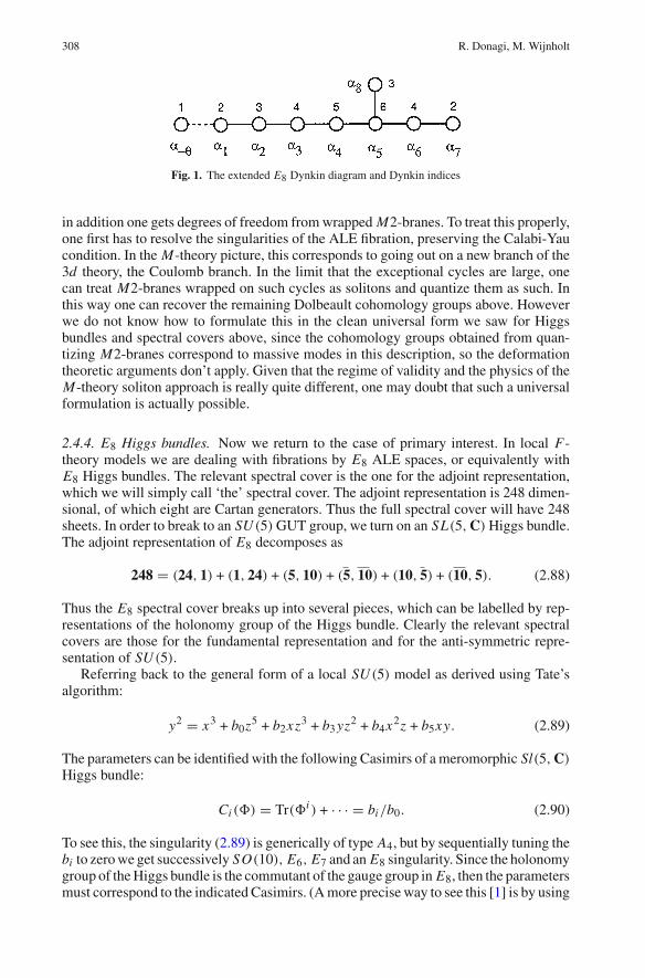
Fig. 1. The extended E8 Dynkin diagram and Dynkin indices
in addition one gets degrees of freedom from wrapped M2-branes. To treat this properly,one first has to resolve the singularities of the ALE fibration, preserving the Calabi-Yaucondition. In the M-theory picture, this corresponds to going out on a new branch of the3d theory, the Coulomb branch. In the limit that the exceptional cycles are large, onecan treat M2-branes wrapped on such cycles as solitons and quantize them as such. Inthis way one can recover the remaining Dolbeault cohomology groups above. Howeverwe do not know how to formulate this in the clean universal form we saw for Higgsbundles and spectral covers above, since the cohomology groups obtained from quan-tizing M2-branes correspond to massive modes in this description, so the deformationtheoretic arguments don’t apply. Given that the regime of validity and the physics of theM-theory soliton approach is really quite different, one may doubt that such a universalformulation is actually possible.
2.4.4. E8 Higgs bundles. Now we return to the case of primary interest. In local F-theory models we are dealing with fibrations by E8 ALE spaces, or equivalently withE8 Higgs bundles. The relevant spectral cover is the one for the adjoint representation,which we will simply call ‘the’ spectral cover. The adjoint representation is 248 dimen-sional, of which eight are Cartan generators. Thus the full spectral cover will have 248sheets. In order to break to an SU (5) GUT group, we turn on an SL(5, C) Higgs bundle.The adjoint representation of E8 decomposes as
Thus the E8 spectral cover breaks up into several pieces, which can be labelled by rep-resentations of the holonomy group of the Higgs bundle. Clearly the relevant spectralcovers are those for the fundamental representation and for the anti-symmetric repre-sentation of SU (5).
Referring back to the general form of a local SU (5) model as derived using Tate’salgorithm:
The parameters can be identified with the following Casimirs of a meromorphic Sl(5, C)
Higgs bundle:
Ci (�) = Tr(�i ) + · · · = bi/b0. (2.90)
To see this, the singularity (2.89) is generically of type A4, but by sequentially tuning thebi to zero we get successively SO(10), E6, E7 and an E8 singularity. Since the holonomygroup of the Higgs bundle is the commutant of the gauge group in E8, then the parametersmust correspond to the indicated Casimirs. (A more precise way to see this [1] is by using
Higgs Bundles and UV Completion in F-Theory 309
the F-theory/heterotic duality map.) We see that there exists a canonical map betweenthe parameters in the ALE fibration, and an SU (5) spectral cover in KS → S defined by
b0s5 + b2s2 + · · · + b5 = 0. (2.91)
Note that η is related to our earlier t by η = 6c1 − t . The five roots {λ1, . . . , λ5} of thispolynomial determine the sizes of all the cycles of the E8 ALE space. Recall that the λiare eigenvalues corresponding to certain eigen-lines,
� |i〉 = λi |i〉 . (2.92)
As discussed in Sect. 5.1 of [5], we can take the five roots of the polynomial to correspondto the periods of the following cycles (up to Weyl permutations)
The sizes of the cycles {α5, . . . , α8} are taken to be zero, generating an SU (5) GUTgroup, and all other cycles are obtained as linear combinations. The matter curve �10corresponds to λi = 0 for some i , the matter curve �5 corresponds to λi + λ j = 0for some i, j , etc. The top Yukawa is localized at λi = λ j = λi + λ j = 0, the bot-tom at λi + λ j = λk + λl = εi jklmλm = 0, and the 5 · 5 · 1 (at least formally) atλi + λ j = λ j + λk = λi − λk = 0.
2.5. Construction of fluxes. Let us briefly recap what we saw above. Local models in F-theory correspond to ALE fibrations over a surface S with G-flux. Physically we expectthat this data, the ALE fibration and the G-flux, can be described as configurations in an8d supersymmetric Yang–Mills theory compactified on S, i.e. a Higgs bundle. This isindeed the case, and moreover this data is also equivalent to a covering CE of the zerosection in an auxiliary non-compact Calabi–Yau threefold X = (KS → S), togetherwith a holomorphic line bundle. In a IIb-like language, we can call this covering a non-compact flavour brane, whose intersection with the gauge brane (which is wrapped onthe zero section of X ) yields the matter curve �10. The group theory of E8 impliesthat there is a second flavour-brane C 2 E , completely determined by the first covering,whose intersection with the gauge brane yields the matter curve �5.
Constructing the branes, or equivalently the ALE fibration, is easy: we only needto specify the bi , which are sections of line bundles on S with Chern classes given byη − ic1. In order to get chiral matter however we must actually turn on a flux on CE ,which will determine a unique flux on C 2 E by group theory. In this subsection wediscuss the issue of constructing such fluxes.
In order to facilitate the analysis we will compactify the local Calabi–Yau to
X = P(O ⊕ KS). (2.94)
X is certainly not a Calabi–Yau; the Calabi–Yau metric diverges at infinity. We denoteby O(1) the line bundle on X which restricts to the eponymous line bundle on eachP1-fiber. We may choose homogeneous coordinates (u1, u2) on the P1-bundle whichare sections of O(1) and O(1) ⊗ KS respectively. The coordinate s used previously isidentified with u2/u1.
310 R. Donagi, M. Wijnholt
The spectral cover C ⊂ X is compactified to a compact surface C ⊂ X by adding adivisor η∞ at infinity. The equation
b0s5 + b2s3 + b3s2 + b4s + b5 = 0 (2.95)
has a double zero at u1 = 0. Therefore η∞ covers η exactly once and is isomorphicto it. We denote the cohomology class dual to the zero section (the Poincaré dual of Sin X ) by s0 and the class of the section at infinity by s∞ = c1(O(1)). Then we haves∞ = s0 + c1(T S) and 0 = s0 · s∞ = s0 · (s0 + c1(T S)).
We would like to lift line bundles on C to line bundles on the compact surface Cwhich are easier to study. If the genus of η∞ is non-zero, then there may be line bundleson C that cannot be lifted to C . However any algebraic line bundle on C can be lifted. Tosee this, any algebraic line bundle on C is of the form O(D)C for some divisor D. LetD be the closure of D in C . Then O(D)C gives a lift of O(D)C as desired. Moreoverglobal G-fluxes are algebraic and yield an algebraic class in the local model. Thereforefrom here on we may restrict our attention to extendable line bundles.
Now consider a spectral line bundle L on C . The corresponding Higgs bundle isgiven by E = pC∗L , � = pC∗s. We have
c1(pC∗L) = pC∗c1(L)− 1
2pC∗r, (2.96)
where r is the ramification divisor, r = −c1(C) + p∗C c1(S). Explicitly we find that
r = (n − 2)s0 + p∗C (η − c1(S)). (2.97)
If c1(pC∗L) is not zero, then we have a GL(n, C) Higgs bundle rather than an SL(n, C)
Higgs bundle. For phenomenological applications we want the latter, so we need toimpose the restriction c1(pC∗L) = 0 on the allowed spectral line bundles. Then it isconvenient to decompose
c1(L) = 1
2r + λγ, (2.98)
where λ is a parameter. The condition c1(pC∗L) = 0 is then equivalent to pC∗γ = 0.The class r/2 is generally not integer quantized. Since c1(L) must be integer quantized,γ must compensate and can generally not be an integer class either, but it will alwaysbe a rational linear combination of integer classes.
So our task is to find integer classes γ with pC∗γ = 0 in H2(C, Z). To get a supersym-metric configuration, γ must further be of Hodge type (1, 1). As we will now argue, forgeneric complex structure moduli there exists only one such class (up to multiplicationby an integer), and we can write it down explicitly.
As for line bundles on C , we can use the Lefschetz–Noether theorem. C is thezero locus of a section of O(n)⊗ Lη−nc1 , which is usually an ample line bundle sinceO(n) is ample and Lη−nc1 is effective and non-zero. Therefore there is an injective mapi∗ : H1,1(X)→ H1,1(C). As a result, H1,1(C) splits into two pieces, the classes inher-ited from X and the primitive classes. The Noether–Lefschetz theorem says that whenC is ample, then for ‘generic’ complex structure moduli there are no primitive classesin H1,1(C).
Let us write down the inherited class explicitly. The cohomology group H2(X , Z) isspanned by s0 and π∗H2(S, Z), i.e. the pull-back of classes on S to X . Therefore theinherited classes in H1,1(C) are spanned by the class of the matter curve �10, as well as
Higgs Bundles and UV Completion in F-Theory 311
any class on S pulled back to C . (In particular, c1(C) is in this span, by the adjunctionformula, and so is η∞.) Our class γ will be a linear combination of those, but it alsoneeds to satisfy pC∗γ = 0, which is clearly not satisfied by any class pulled back fromS. Thus we can single out the class [�E ] and subtract the ‘trace’, i.e. we single out thefollowing unique linear combination:
We used the subscript u on γu to indicate that this class is universal, i.e. it always existsin a local model. In the last equality we just use the fact that pC∗[�E ] is just the class[�E ] sitting inside H2(S), and since it is given by bn = 0 it follows that it can also bewritten as η − nc1.
Let us define a line bundle using this class. Its first Chern class will be given by
c1(L) = 1
2r + λγu, (2.100)
with γu as defined above and λ a parameter. From our explicit expressions for r andγu , we see that c1(L) is an integer class when λ is an integer and n is even, or whenλ = 1
2 + integer and n is odd. For this corresponding choice of spectral line bundle, wecan deduce the net amount of chiral matter. It is given by
Nchiral = −χ(i∗OS, j∗L) = +χ(L ⊗ KS|�10) = λ
∫
�
γu, (2.101)
where in the last equality we used the Riemann–Roch formula and the fact that(r/2 + c1(KS))|� = −c1(�)/2. We have
� ·C � = S0 ·X S0 ·X C = −c1(S0) ·S0 �. (2.102)
Further we have � ·C p∗α = α ·S0 � for any α ∈ H2(S, Z). Applying this withα = η − nc1, we see that
γu ·C � = −η ·S0 �. (2.103)
Therefore we find
Nchiral = λ
∫
�
γu = −λη(η − nc1). (2.104)
This is of course the same formula as encountered in spectral cover constructions in theheterotic string [40].
Therefore the only fluxes available for general complex structure moduli will givethe conventional chirality formula known from the heterotic string. We do not see moregeneral options in the local F-theory set-up. We will call such fluxes inherited or uni-versal. However, there do exist more general fluxes, both in the heterotic setting andin the F-theory setting. The point is that general fluxes are not supersymmetric forgeneric Higgs bundle moduli, and thus are not among the fluxes that we found above.For special values of the moduli (which is called the Noether–Lefschetz locus) there areadditional supersymmetric fluxes available, and turning on such fluxes would thereforeautomatically stabilize some of the moduli. We will call them Noether–Lefschetz fluxesor non-inherited fluxes. Generic fluxes are non-inherited. They exist for both F-theoryspectral covers and heterotic spectral covers, where they give rise to rigid bundles onthe CY3 after Fourier–Mukai transform. But they are harder to write down and have notreally been analyzed in either context.
312 R. Donagi, M. Wijnholt
2.6. Further constraints. In the previous sections we encountered a number of con-straints that must be satisfied for consistency of the local model. Now we would like toconsider imposing a few further constraints, that are not needed for consistency but arelikely needed to get a realistic and calculable four-dimensional model. We will concen-trate on SU (5) models, so there is a matter curve
[�10] = c1 − t, (2.105)
which must be effective and non-zero.The Kähler class J is a generator of H2(B3, R) that must be positive on all the effec-
tive cycles of the geometry. Modulo these positivity constraints, there is an independentscale in the geometry for every generator of H2(B3, R). In order to get a model that iscalculable and predictive, we need some small parameters that we can expand in. Themain requirement that we want to make is that MGU T /MPl is unbounded from below,where MGU T ∼ V−1/4
S and MPl ∼ V 1/2B3
/κ ∼ V 1/2B3
/αGU T VS .Now although MGU T /MPl → 0 should make gravity subleading, it may not be
enough to decouple the local model. Depending on the geometry of B3, there may beadditional scales in the global model with physics that cannot be decoupled from thevisible sector. In order to say that the visible sector is largely independent of the restof B3, we will want to require that one can take VS → 0 while keeping VB3 as well asthe volume of any other cycles not inside S finite. This implies that the kinetic terms offields localized on any cycle not contained in S are large compared to the kinetic termsof the fields localized on S. Moreover this yields a local constraint that can be checkedwithout knowing the compactification manifold B3.
There are two ways in which we could take VS → 0 while keeping other cycles fixed.The first is that we could require S to contract to a point. This will turn out to be a verystrong condition which will essentially single out a unique model. We could also requireS to contract to a curve of singularities. This is a less stringent condition, but togetherwith some other physical constraints will still rule out a good deal of models.
Thus our first assumption is as follows:
1. Contractibility. S can be contracted to a point. By Grauert’s criterion [41], this meansthat the class t must be ample, in particular t · C > 0 for any curve C in S.5
We can draw some immediate conclusions from this assumption. Since c1− t is effectiveand non-zero, and t is ample, c1 must be effective and non-zero. Therefore K−n
S cannothave sections for any positive n and the Kodaira dimension is−∞. From the classifica-tion of surfaces, we then know that S is related to P2 or a ruled surface (i.e. a P1-fibrationover a Riemann surface of genus g) by a sequence of blow-ups and blow-downs.
The ruled surfaces have h1,0(S) = g, which would lead to massless adjoint fields inthe effective four-dimensional theory if g > 0. This looks phenomenologically undesir-able, so we will exclude this possibility with our second assumption:
2. No adjoint scalars. The Hodge numbers of S must satisfy h0,1(S) = 0 andh2,0(S) = 0.
Then S is either P2 or can be obtained by a sequence of blow-ups from a Hirzebruchsurface Fr . Note this includes all the del Pezzo surfaces. The divisors on Fr are generatedby b, f and Ei , with the intersection numbers
5 Even though we have seen that for many purposes S can be regarded as living inside the total space ofthe canonical bundle, this criterion has nothing to do with contractibility in the auxiliary local Calabi-Yau. Wewill see this more explicitly in the global examples later.
Higgs Bundles and UV Completion in F-Theory 313
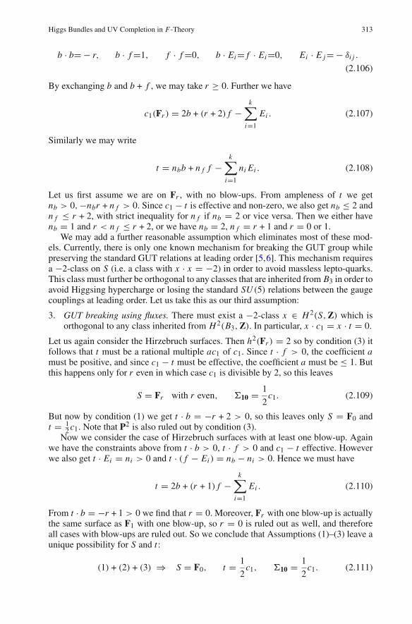
b · b=− r, b · f=1, f · f=0, b · Ei= f · Ei=0, Ei · E j=− δi j .
(2.106)
By exchanging b and b + f , we may take r ≥ 0. Further we have
c1(Fr ) = 2b + (r + 2) f −k∑
i=1
Ei . (2.107)
Similarly we may write
t = nbb + n f f −k∑
i=1
ni Ei . (2.108)
Let us first assume we are on Fr , with no blow-ups. From ampleness of t we getnb > 0,−nbr + n f > 0. Since c1 − t is effective and non-zero, we also get nb ≤ 2 andn f ≤ r + 2, with strict inequality for n f if nb = 2 or vice versa. Then we either havenb = 1 and r < n f ≤ r + 2, or we have nb = 2, n f = r + 1 and r = 0 or 1.
We may add a further reasonable assumption which eliminates most of these mod-els. Currently, there is only one known mechanism for breaking the GUT group whilepreserving the standard GUT relations at leading order [5,6]. This mechanism requiresa −2-class on S (i.e. a class with x · x = −2) in order to avoid massless lepto-quarks.This class must further be orthogonal to any classes that are inherited from B3 in order toavoid Higgsing hypercharge or losing the standard SU (5) relations between the gaugecouplings at leading order. Let us take this as our third assumption:
3. GUT breaking using fluxes. There must exist a −2-class x ∈ H2(S, Z) which isorthogonal to any class inherited from H2(B3, Z). In particular, x · c1 = x · t = 0.
Let us again consider the Hirzebruch surfaces. Then h2(Fr ) = 2 so by condition (3) itfollows that t must be a rational multiple ac1 of c1. Since t · f > 0, the coefficient amust be positive, and since c1 − t must be effective, the coefficient a must be ≤ 1. Butthis happens only for r even in which case c1 is divisible by 2, so this leaves
S = Fr with r even, �10 = 1
2c1. (2.109)
But now by condition (1) we get t · b = −r + 2 > 0, so this leaves only S = F0 andt = 1
2 c1. Note that P2 is also ruled out by condition (3).Now we consider the case of Hirzebruch surfaces with at least one blow-up. Again
we have the constraints above from t · b > 0, t · f > 0 and c1 − t effective. Howeverwe also get t · Ei = ni > 0 and t · ( f − Ei ) = nb − ni > 0. Hence we must have
t = 2b + (r + 1) f −k∑
i=1
Ei . (2.110)
From t · b = −r + 1 > 0 we find that r = 0. Moreover, Fr with one blow-up is actuallythe same surface as F1 with one blow-up, so r = 0 is ruled out as well, and thereforeall cases with blow-ups are ruled out. So we conclude that Assumptions (1)–(3) leave aunique possibility for S and t :
(1) + (2) + (3) ⇒ S = F0, t = 1
2c1, �10 = 1
2c1. (2.111)
314 R. Donagi, M. Wijnholt
We will study this case in more detail later in the paper. In particular we will show howto engineer three-generation models and how to embed it in a global model.
It is evident by now that condition (1) in particular is quite strong. In order to haveVS → 0 while keeping other cycles fixed, we can also replace assumption (1) by:
1′. Contractibility. S can be contracted to a curve, i.e. S admits a fibration F → S→ Bwhere the fibers F can be contracted to a curve B of singularities.
In this case t is not necessarily ample, but t must be ample when restricted to the com-ponents that are being contracted [42,43]. Therefore, t · C > 0 when C is the generalfiber F or an irreducible component of the singular fibers.
A priori the base B of the fibration can have any genus g, in which case we wouldhave h1,0(S) = g. Again by assumption (2) the base B is restricted to be P1. Likewise,the fibers must be rational: the curve c1 − t = �10 is effective and the fiber F moves,so there must be some copy of F that is not contained in �10. Therefore we must have(c1−t)·F ≥ 0. Since F gets contracted, we have t ·F > 0, and it follows that c1 ·F > 0.But by the adjunction formula we have c1 · F = 2− 2g(F), hence c1 · F = 2 and F isa P1 as promised.
So our S is a ruled surface with rational base and fibers. From the classification ofsurfaces, we know that S is rational and can be obtained by blowing up some pointson a Hirzebruch surface Fr . The most general possibility is obtained by blowing upsome points on a conic bundle, which allows for the possibility of a multiple fiber. Ourargument below is actually even more constraining when there are multiple fibers, so inwhat follows we will focus on the case that none of the fibers is multiple.
If S is a Hirzebruch surface then we can run the previous argument. Using condition(3) it follows that t = 1
2 c1 and r is even. Apart from these we must consider possibleblow-ups of Fr . Again we write
t = nbb + n f f −k∑
i=1
ni Ei . (2.112)
Under assumption (1′) we can no longer conclude that t · b must be positive, but we stillknow that t must be positive on f, Ei and f − Ei . From t · f > 0, t · Ei > 0 andt · ( f − Ei ) > 0 we get nb > 0, ni > 0, and nb − ni > 0. From c1 − t effective andnon-zero we get nb ≤ 2 and n f ≤ r + 2, with strict inequality for n f if nb = 2 andni = 1. Therefore the only possibility is
S = Bk(Fr ), t = 2b + n f f −k∑
i=1
Ei , �10 = (r + 2− n f ) f (2.113)
with n f < r + 2. Here we used Bk to denote blowing-up k times. These possibilities alsosatisfy condition (3), since there are classes of the form f − Ei − E j and Ei − E j whichare orthogonal to c1 and t . Moreover we can’t do too many blow-ups. Recall that thesections bi specifying an SU (5) model live in c1− t, . . . , 6c1 − t , so these line bundlesneed to admit sections.
So we conclude that under assumptions (1′), (2) and (3), we get the following possi-bilities for S and t :
S = Fr with r even, t = 1
2c1, �10 = 1
2c1 (2.114)
Higgs Bundles and UV Completion in F-Theory 315
or
S = Bk(Fr ), t = 2b + n f f −k∑
i=1
Ei , n f < r + 2. (2.115)
The remaining possibility S = P2 is still ruled out by assumption (3).We may consider adding one final assumption. We will soon see though that this
assumption has a very important loophole, so it will be weakened significantly.
4. Three generations. The net number of generations is given by
− λ(6c1 − t) ·d P (c1 − t), (2.116)
where λ ∈ Z + 12 . As we argued, this is the only universal formula one can write
down. However this does not represent the most general configuration of local F-theory models and will be revisited in Sect. 2.8.
Let’s apply this to all the possibilities we found. For the Hirzebruch surfaces with t = 12 c1
we find that the minimal number of generations is eleven. For the blow-ups of Hirze-bruch surfaces with t as in (2.115), we find that the minimal number of generations is5× (r + 2−n f ), and in general it is always divisible by 5. We conclude it is not possibleto make a local three generation SU (5) model under these assumptions.
If we drop condition (1) or (1′) it is not hard to find three-generation models. Forinstance, the d P8 example in [1] with η = 6c1(S) is consistent and satisfies assumptions(2) and (3), but it does not satisfy assumption (1) or (1′) since it has t = 0, and istherefore not a truly local model.
It may be interesting to point out that the three generation SO(10) models in [1](which have η = 4c1 + E , where E is any −1-curve, and �16 = [E]) do satisfy theconditions (1),(2) and (3) for d Pk with 2 ≤ k ≤ 7. However a fully satisfactory wayof breaking the SO(10) GUT group in these models while preserving gauge couplingunification has not yet been identified. (This has recently been revisited in [44], whereit was shown that one can actually use hypercharge flux without introducing exotics.)
To summarize this subsection, under conditions (1) – (3) we only found one pos-sibility for S and t , listed in (2.111). Under assumptions (1′) – (3) we only found thepossibilities listed in (2.114) and (2.115). Using the inherited fluxes (assumption (4)),none of these models could account for three generations. In the following subsections,we will examine some possible loopholes in our assumptions.
2.7. Another way to break the GUT group. In [5,6] the GUT group was broken to theStandard Model gauge group by turning on an abelian flux. A priori there exists a secondpossibility: one may also break the GUT group to the Standard Model by turning on anabelian Higgs field.
To do this, we take a degree six spectral cover
b0s6 + b2s4 + · · · + b6 = 0 (2.117)
which generically breaks E8 to SU (3)× SU (2). Note that b1 must vanish if the struc-ture group is to be in SU (6) rather than U (6). Now if the bi are such that this equationfactorizes
(c0s + c1)(d0s5 + d1s4 + · · · + d5) = 0, (2.118)
316 R. Donagi, M. Wijnholt
where c0d1 + c1d0 = 0, then the structure group of the Higgs field commutes withSU (3)× SU (2)×U (1).
The matter curves are easy to find. Consider first an irreducible degree 6 spectralcover (this was worked out in [3]). One uses the following decomposition of the adjointof E8 under SU (3)× SU (2)× SU (6):
In the reducible case we simply substitute the bi for the appropriate bilinears in ci and d j .In addition there can be hypercharged scalars. To see this, recall that the moduli of
the spectral cover are counted by
Ext1X (i∗L , i∗L). (2.121)
When the spectral cover is reducible, this decomposes as∑
m,n
Ext1X (im∗Lm, in∗Ln), (2.122)
where m, n run over the irreducible components. The off-diagonal zero modes are clearlycharged under the extra U (1)’s since their VEVs smooth the spectral cover and breakthese U (1)’s. These modes are localized at the intersection c0s+c1 = d0s5+d1s4+. . .+d5.In order to get a realistic model, such hypercharged scalars must be absent, and we haveto pick a spectral line bundle which ensures that.
There are unfortunately at least two possible issues with this scenario. The polynomialb6 is a section of NS . Thus not only c1− t should have a section, but also−t . By our clas-sification of the possible pairs (S, t), even with condition (3) dropped, such an S can notbe contractible, which means it is not a true local model. Thus this mechanism can onlybe used if we drop the requirement that MGU T /MPl can be made parametrically small.
The second issue is that since we are in some sense directly breaking E8 toSU (3) × SU (2) × U (1)Y , it is not guaranteed that the gauge couplings will unify.This could perhaps be addressed by requiring c1/c0 to be small, as the spectral coverdegenerates and the breaking of SU (5)GU T to the Standard Model gauge group shouldbe small in the limit c1/c0 → 0.
2.8. Noether–Lefschetz fluxes. The results of Sect. 2.6 clarify our options. Dropping thefirst assumption is a priori possible and leads to consistent models, but it would meanwe can not make an expansion in MGU T /MPl and therefore would greatly diminishthe predictiveness of F-theory GUTs. Dropping assumption (3) means that we needan alternative mechanism to break the GUT group while preserving the standard SU (5)
relations at leading order. We made such an alternative proposal in Sect. 2.7 but it did notseem to be compatible with contractibility of S. Therefore we are led to drop assumption(4) and investigate the possibilities of non-inherited G-fluxes.
Higgs Bundles and UV Completion in F-Theory 317
The argument in Sect. 2.6 that the inherited fluxes are not sufficient by no means rulesout three generation models. Rather it means that we need to look at more general fluxesthat are not critical points of the holomorphic Chern–Simons superpotential for genericmoduli, and we have to do more work to show that there exists a stable supersymmetricminimum. In mathematics circles this would be called a Noether–Lefschetz problem. Onthe other hand, the first three assumptions already ruled out all but a handful of 7-braneconfigurations, listed in (2.111), (2.114) and (2.115) in Sect. 2.6. Thus in contrast to eg.heterotic model building, we have a very restricted set of possibilities to start with andwe know all the continuous parameters.
Let us first ignore the requirement of supersymmetry, and simply ask if there are anyfluxes available, not necessarily of type (1, 1), which might give three generations. Thiswill be the case if we can show there exists a class γ2 ∈ H2(C, Z) which is orthogonal top∗C H2(S, Z) and satisfies γ2 ·�10 = 1, since then we can add some integer multiple ofit to 1
2r + 12γu and get any number of generations we want. Equivalently, γ2 must satisfy
γ2 · γu = γ2 · (5�10 − p∗C pC∗�10) = 5. (2.123)
Now the lattice H2(C, Z) modulo torsion is unimodular by Poincaré duality. Thus if γuis primitive in the sense that it is not an integer multiple of a smaller integer class, thenthere exists an α ∈ H2(C, Z) such that
α · γu = 1. (2.124)
Then defining γ2 = 5α − p∗C pC∗α, we have γ2 · γu = 5 and pC∗γ2 = 0 as required.Therefore we are guaranteed that the required fluxes exist if γu is primitive in the senseabove. In a unimodular lattice, a sufficient condition is that γu · γu is not divisible byany square. It is easy to see that γu · γu = 5γu ·�10 which we have already computed inSect. 2.6. For S = P1 × P1 with t = 1
2 c1, it is equal to 5× 22 which does not have anysquares. So we conclude from a purely topological argument that it is possible to obtainthree generations, although this argument cannot establish that there is a supersymmetricminimum for finite values of the Higgs bundle moduli.
In the following we would like to give a fairly general construction of algebraicclasses that satisfy α ·C γ = 1. We will apply it to S = P1 × P1, but it should beclear that with some simple substitutions it can also be applied to the other cases. Thuswe will finally establish some examples of supersymmetric SU (5) models with threegenerations and S contractible.
The strategy is as follows: we first take a curve α0 ∈ H2(S, Z) such that α0 ·S�10 = 1.Then we will construct a curve α ∈ X which does not intersect �10, and which covers α0exactly once. Finally we will require C to contain α by tuning the complex structure mod-uli. The result is an algebraic class in H2(C, Z) with α ·C γ = 1. We can then construct anadditional flux γ2 as above by subtracting the trace, and define a spectral line bundle with
c1(L) = 1
2r +
1
2γu + nγ2. (2.125)
By adjusting n, we then get any number of generations we want.In the case of interest, we have S = P1 × P1. We denote the coordinates on
S by (z1, z2;w1, w2), and the two rulings by H1 and H2, with intersection numbersH2
1 = H22 = 0, H1 · H2 = 1. As we deduced above, the matter curve should be given
by �10 = [H1 + H2], and we need a class with α0 · �10 = 1. Thus a simple choice isto pick α0 = H1, though clearly there are additional options. In equations it is given by(say) w1 = 0.
318 R. Donagi, M. Wijnholt
Now we need to construct α. As before we use coordinates (u1, u2) on the P1-fibersof X = P(O ⊕ KS). Then we define α by the following two equations:
α : w1 = 0, u1 = P2(z, w)u2, (2.126)
where P2(z, w) is a section of O(2, 2). Note that u2 = 0 ⇒ u1 = 0, so α does notintersect the zero section u2 = 0. This is needed if we want C to contain α, because theintersection of C with u2 = 0 is by definition �10, and we promised to construct a classwhich does not intersect �10. Also, α covers α0 precisely once.
Therefore we now need to show that we can tune the complex structure moduli sothat C contains α. The equation of C is given by
b0(z, w)u52 + b2(z, w)u2
1u32 + · · · + b5(z, w)u5
1 = 0. (2.127)
We simply substitute the equations for α in order to get a restriction on the coefficientsof C . Clearly we find that
The only thing left to check is that C is generically smooth, so that our calculations ofthe chiral spectrum apply. But this is fairly obvious because generically the derivativesof Eq. (2.127), even with (2.129), give independent equations.
Therefore we have constructed a (1, 1) class γ2 = 5α − p∗C pC∗α with the desiredproperties. Defining a spectral line bundle as in (2.125) with n = 8, we find preciselythree chiral generations on �10.
2.9. ‘Flux’ landscapes in the heterotic string and F-theory. As we already remarked,much of the structure of F-theory vacua is identical with that of the heterotic string. BPSinstantons effects, branes and flux superpotentials, which are some of the main ingredi-ents inducing potentials for the moduli, can be related under the duality. In particular,semi-realistic heterotic models appear to have an enormous number of ‘flux’ vacua aswell. We put ‘flux’ in quotation marks here because after Fourier–Mukai transform, weget a smooth non-abelian bundle on the Calabi–Yau threefold without any U (1) fluxes.These extra ‘flux’ vacua are obtained by using spectral line bundles that are not inherited,and generically should stabilize all vector bundle moduli. There is a landscape of suchvacua and a priori it is not clear why we should exclude these possibilities. The methodwe used for constructing such more general fluxes in Sect. 2.8 can also be used in theheterotic string.
Thus landscapes seem to be quite generic properties of superpotentials in string the-ory. It would be interesting to study these vacua microscopically. In the heterotic settingthere are no RR fields so one could try to use conventional CFT techniques. Perhaps onemay then find a reason to exclude most of them, although it is currently not clear whythat would be the case.
As in type II settings, this leads to philosophical problems: we don’t really understandmoduli stabilization and the cosmological constant problem very well, it is practicallyimpossible to enumerate all the vacua that seem to exist at the effective field theory
Higgs Bundles and UV Completion in F-Theory 319
level, and one of the solutions that have been proposed to solve the cosmological con-stant problem is NP hard [45]. A possible way out was promoted in [46]: if M/MPl canbe parametrically small, where M is some scale relevant for particle physics like theGUT scale, then we can prevent the unknown physics responsible for solving gravity-related problems from feeding back into physics at the scale M . This may allow us todiscuss phenomenology without having to solve the cosmological constant problem andother problems related to gravity. But combining this principle with GUTs leads us toF-theory; this idea cannot be implemented in the heterotic string.
2.10. Conclusions. We have clarified the rules for constructing local models in F-theory.Such models can be defined by specifying suitable spectral data (a type of B-brane) in anauxiliary Calabi–Yau geometry. We classified the possible matter curves for local SU (5)
models. We have constructed the first truly local SU (5) models with three generations.We did not compute the exact matter content in our model, so it is possibly still an openproblem to construct local SU (5) models with exactly the MSSM spectrum, or someacceptable extension. However since it is now clear that there is a landscape already inlocal models, and since there is no index theorem that prevents chiral/anti-chiral pairsfrom lifting, we should expect the number of models with the MSSM spectrum to beenormous.
We explained how to connect F-theory models to a IIb picture by taking an orien-tifold limit. For SU (5)GU T models, it was found that the E6 points on S where theup-type 10 · 10 · 5 Yukawa couplings are localized became singular points in the pertur-bative IIb limit. However a number of general issues pertaining to the IIb limit remainedunresolved. A much better approach to this problem will be presented in [21].
We also found that it seems to be impossible for a local SU (5) model with com-pletely unstabilized Higgs field moduli to have three generations. From a physical per-spective, this is good news since there are many indications that we do not want ageneric model, such as problems associated to dimension four and five proton decay.Thus requiring a three-generation model automatically stabilizes some of the moduli.Requiring the precise MSSM spectrum will likely stabilize even more moduli. On theother hand, this also makes the problem of constructing realistic local models much morechallenging.
Along the way we have encountered a number of constraints that the matter curvesand fluxes on the matter curves must satisfy in a consistent local model, from topologicaland integral (such as anomaly cancellation (2.29) and the fact that the flux must lift tothe integral class of a line bundle L with c1(pC∗L) = 0), to analytic (such as the forcedsingularities on � 2 E and constraints on the moduli entering the matter curves for non-inherited fluxes, so that L is a holomorphic line bundle). Probably we have not foundthem all, since some of these constraints look very non-trivial from the point of view ofthe brane carrying the unbroken gauge group. However we have shown that there is anisomorphism relating a configuration (E,�) in the 8d gauge theory to its spectral data(CE , L E ), and the constraints on the spectral data are few and simple to understand.
In the next section we will make the first strides towards embedding our local modelsin a global model.
3. Compactification
In order to get a finite four-dimensional Planck scale we should embed our local modelsinto a compact elliptically fibered CY fourfold. In the philosophy of local model build-
320 R. Donagi, M. Wijnholt
ing, the goal of this pursuit is not to find ‘the’ UV completion of the local model. Indeedas we reviewed earlier, it is not even clear that this is an answerable question. Rather it isto ascertain that all the ingredients used can in principle be combined in a UV completemodel, and there are no obvious constraints from UV completion that would rule themout.
In doing so there are many issues to be addressed. Our aim here is rather modest;we would like to discuss a simple set of compactifications which implement a few ofthe requirements for viable local GUTs, and which make clear how such constructionswork in general. In particular we would like to construct compactifications in whichGUT breaking by fluxes can be implemented, and in which dangerous proton decaychannels can be avoided.
Our discussion will have one important caveat. We will freely assume that appropriatefluxes may be found which give precisely the Standard Model spectrum on the mattercurves we engineer. The point of our discussion is not to understand the fluxes, but rathersome of the constraints on the geometry of the four-fold arising from phenomenologicalrequirements.
3.1. First example: cubic surface in P3. Let us discuss simple compactifications of localtoy models with SU (5) GUT group. Our GUT brane should be wrapped on a Del Pezzosurface S2 ⊂ B3, such that some homology classes in the Del Pezzo become boundarieswhen embedded in B3. For simplicity we will take B3 to be P3 in our first example,although much of what we will say can clearly be adapted to more general Fano three-folds. Then we can take S2 to be a quadric surface Q2(z1, z2, z3, z4) = 0 (i.e. P1 × P1)or a cubic surface Q3(z1, z2, z3, z4) = 0 (i.e. a Del Pezzo 6). For definiteness we takethe cubic.
Recall again the Tate form of the Weierstrass equation,
y2 + a1xy + a3 y = x3 + a2x2 + a4x + a6, (3.1)
where the ai are sections of K−iB3
. In the case of B3 = P3, the ai are polynomials ofdegree 4i . As we discussed, in order to get an I5-locus along Q3 = 0, as well as mattercurves and Yukawa coupling localized along certain prescribed submanifolds, we mustimpose certain restrictions on the ai which can be read from Table 1.
Now let us try to impose various constraints.
1. SU (5) gauge group on Q3 = 0. According to Table 1 this implies the followingleading form for the ai :
where s = Q3 and the Pn are generic polynomials of degree n on P3. They areidentified with the sections b9−n that appeared in the general discussion. In factwe are clearly allowed to add further subleading terms, eg. a1 = P4 + sT1, a2 =s P5 + s2T2, et cetera. Such additional subleading terms do not affect behaviour nearthe I5 locus, but they do provide additional flexibility in building a global model. Tokeep things simple, we will set them to zero. Then the discriminant is computed to be
� = s5 P44 (−P9 P4
2 + P6 P7 P4 − P5 P62) + O(s6), (3.3)
which vanishes to 5th order along Q3 = 0, as required.
Higgs Bundles and UV Completion in F-Theory 321
2. Matter curves. The discriminant vanishes to higher order along �10={Q3= P4=0}and �5 = {Q3 = R17 = 0}, where
R17 ≡ P9 P42 − P6 P7 P4 + P5 P6
2. (3.4)
Note that
2TQ3 = O(1)|Q3 , NQ3 = O(3)|Q3 (3.5)
and hence the cohomology classes dual to �10 and �5 on Q3 are given by c1 − tand 8c1 − 3t . Of course this all fits in the general discussion in Sects. 2.1 and 2.3.
3. Yukawa couplings and dimension four proton decay. The up-type Yukawa couplingsare localized at {Q3 = P4 = P5 = 0} and the down type Yukawas are localized at{Q3 = P4 = P6 = 0}. Methods for suppressing proton decay in F-theory were dis-cussed in [5,6,30]. Here we will see how they can be implemented in global models.In order to prevent dimension four proton decay, we want to make sure that
The coupling 10m · 5h · 5h will be absent automatically due to the anti-symmmetry.We will try to implement the above by splitting �5 into two pieces, one supportingthe matter fields and another supporting the Higgses. This means we have to tunethe Pn so that the polynomial R factorizes modulo Q3. In terms of ideals, we requirea decomposition
〈Q3, R〉 = I5m∩ Ih . (3.7)
To secure the absence of R-parity violating down-type Yukawa couplings we mustmake sure that whenever we have an intersection of �10m with �5m
, there is alsoa branch of �5h
intersecting at that point. Since R = 0 has a double point at suchintersections, we can also say that whenever �10m intersects with �5m
, then �5mis
not allowed to have a double point (the second order vanishing of R instead being dueto a branch of �5h
coming in and intersecting there). Similarly in order to avoid the
couplings 10m ·5h ·5h , we want to avoid double points on �5hdwhich also meet �10m .
We don’t know the general solution to this algebraic problem. But to see that it canbe achieved, we will exhibit one simple solution that exists for more general SU (5)
models as well. We take
P6 = Hd6 mod Q3, P9 = Hu
1 T2 Hd6 mod Q3,
P7 = Hu1 T6 mod Q3, P5 = Hu
1 T4 mod Q3,(3.8)
for some Ti and Hi of the appropriate degree, but otherwise arbitrary. Then we take�5h = {Q3 = Hu
1 Hd6 = 0}, i.e. the Higgs curve is actually reducible, with only up
type Yukawa couplings on Hu1 = 0 (since Hu
1 = 0 implies P5 = 0) and only downtype Yukawa couplings on Hd
6 = 0. When we discuss dimension five proton decaywe will see why that is a good thing to have. Now we can factorise �5 as
and M10 has no double points at Q3 = P4 = P6 = 0. Moreover the up anddown-type Yukawa’s are still present. For instance the up-type Yukawa’s come fromQ3 = P4 = Hu
1 = 0, which consists of 3 · 4 · 1 = 12 points.
322 R. Donagi, M. Wijnholt
There are additional cubic couplings of the form
5m · 5hu · 1, 5hd · 5hu · 1. (3.10)
The singlets correspond to Higgs field moduli (which are complex structure moduliof the Calabi–Yau fourfold). At least three of them should give rise to right-handedneutrinos, with the first coupling in (3.10) corresponding to the usual Yukawa cou-plings for neutrinos. The number of moduli appearing in such couplings is thedifference between the number of moduli describing �5m
and �5huseparately or
as a single smooth curve, which yields 65 singlets in our example. The problem ofgetting Majorana masses of the right order of magnitude is a problem of modulistabilization for the Higgs fields. The couplings on the right give rise to the min-imal extension of the MSSM with a dynamical μ-parameter. There are additionalconstraints from dimension five proton decay however, as we discuss next.
4. Dimension five proton decay. We further want to eliminate dimension five protondecay. This proceeds through mediation of massive KK triplets Tu, Td propagatingon curves supporting a hypermultiplet in the 5. The possible channels are given by
Q Qλu←→ Tu
mab←→ Tdλd←→ Q L
�10m �10m �a5 �b
5 �10m �5m
. (3.11)
In order to prevent such processes, we have to shut off at least one of the interactionsin this chain. If Hu and Hd propagate on the same matter curve, and if we assumethe existence of classical up-type and down-type Yukawa couplings for the Stan-dard Model, then such decays are unavoidable. Since we want to keep the classicalYukawa couplings, we require the existence of a decomposition
Ih = Iu ∩ Id , (3.12)
so that we can shut off the coupling mab. If we allow �u and �d to intersect, thenthere could either be a branch of �10m also intersecting there; or it can correspond toa 5u · 5d · 1 coupling. As long as the VEV of the singlet vanishes we do not have thetroublesome mass terms linking triplets localized on �u and �d . In either case theexistence of a classical μ-term is excluded. Our example corresponds to the lattercase: there are 3 · 1 · 6 = 18 intersection points on Hu
1 = Hd6 = 0 corresponding to
the couplings 5u · 5d · 1.There are several possible alternate channels for dimension five proton decay (3.11).The most dangerous are cases where �a
5 = �b5 , because then mass terms mab
between Tu and Td cannot be avoided. The case �a5 = �b
5 = �5mis harmless by
the solution to dimension four proton decay, which shuts off the interactions λd .The case �a
5 = �b5 = �5hd
requires shutting off the interactions λu . The curve�10m is positive in our example and therefore certainly intersects �5hd
. Howeverin our solution to the dimension four problem, by design any such intersection hasP4 = P6 = 0 and therefore corresponds to a λd coupling, not a λu coupling, so thischannel is not available. Finally there is the case �a
5 = �b5 = �5hu
, which requiresshutting off the interaction λd . In our example, by design any intersection pointbetween �5hu
and �10 yields an up-type Yukawa, so the potentially troublesomeinteractions are again absent.The remaining possible channels have �a
5 = �b5 . Assuming both the λu and λd
couplings are present (which they need not necessarily be), the problem is to shut
Higgs Bundles and UV Completion in F-Theory 323
off the interactions mab. This depends on the existence of intersections of �a5 and
�b5 which give rise to a coupling 5 · 5 · 1. If such intersections are present, mab
is proportional to the VEV of the singlet, which is a complex structure modulus.As long as the dynamics of moduli stabilization is such that the VEV of this fieldremains zero, there will be no proton decay through this channel.Consider for instance �a
5 = �5mand �b
5 = �d (the other cases being similar). Thecurves �5m
and �d can intersect in two ways. Either there is also a branch of �10intersecting there, which corresponds to the down type Yukawas that we want tohave; or it corresponds to a 5 · 5 · 1 coupling. In our example with Ihd =
⟨Q3, Hd
6
⟩,
intersection points where Hd6 = 0 and M10 = 0 have either P4 = 0 or T2 P4−T6 = 0.
In the former case it meets with �10, and there are 3 · 6 · 4 = 72 such intersectionpoints; in the latter case it corresponds to the coupling to singlets whose VEV mustremain zero, and this accounts for 3 · 6 · 6 = 108 intersection points.
Hence we see in this simple example that there seems to be enough room in complexstructure moduli space to implement our geometric requirements for absence of dimen-sion four and five proton decay. This is perhaps a little misleading, because we have notcarefully examined the fluxes. When we take the hypercharge flux into account, we findthe following problem. In order to get just the Higgses on �Hu and �Hd and no lighttriplets, the hypercharge flux through these curves should be non-zero and opposite. How-ever the homology classes of the curves above are always pull-backs of homology classesin the bulk, and so the hypercharge flux through them must vanish, if we are to avoidgiving a mass to the hypercharge gauge boson through a Stückelberg coupling to axions.
This problem could be circumvented in general by a slight variation of the factoriza-tion above. With the notation in Sect. 2, the matter curves are given by
where b4|Q3=0 = h·γ . Then it is not hard to see that in general one may have non-zero andopposite hypercharge flux through �Hu and �Hd . If moreover there are no simultaneouszeroes for b5 and γ , then the above arguments for avoiding proton decay still go through.
An alternative approach would be to implement the approach of [30], which requiresdecomposing the SU (5) Casimirs into those of a smaller holonomy group, so that onehas additional U (1) symmetries available.
3.2. Second example: a contractible P1 × P1. In our previous example the del Pezzowas not contractible in B3. The main purpose of this subsection is to give a simpleexample of a del Pezzo S which has two-cycles not inherited from B3 (necessary forallowing GUT breaking fluxes), and which is also contractible in B3. This is an explicitrealization of case (2.111) discussed in Sect. 2.6.
The example is as follows. We will take B3 to be the blow-up of P3 along a curve Cdefined by
C = {Q2 = 0} ∩ {Q3 = 0}. (3.15)
324 R. Donagi, M. Wijnholt
The corresponding ideal is denoted as IC and the blow-up along this ideal as B3 = P3.We have
KP3 = i∗KP3 + C, (3.16)
where C is the exceptional divisor (a P1-fibration over C , given by projectivising thenormal bundle). Sections of the anti-canonical bundle K−1
P3 are sections of K−1P3 which
are also in the ideal IC . In particular there are non-trivial sections in K−4P3 and K−6
P3 , and
so we can write a Weierstrass equation and construct elliptic fibrations over P3 whichare Calabi-Yau.
In this example, the del Pezzo on which the gauge branes are wrapped will be theHirzebruch surface F0 = P1 × P1, here defined by Q2 = 0. As mentioned, the reasonfor picking this model as our next example is that the proper transform of S = {Q2 = 0}is contractible. To see this, let us first check that the normal bundle is indeed negative.The normal bundle of S in P3 is O(2)|S . After blowing up C , the new normal bundle isO(2)|S ⊗O(−C)|S , where C is the exceptional divisor. But the intersection of C withS is in O(3)|S , so
O(2)⊗O(−C)|S ∼ O(−1)|S . (3.17)
Hence the normal bundle is negative, a necessary condition for being contractible.By looking at this example slightly differently, one may establish that S is indeed
contractible. Consider a cubic hypersurface Q in P4 vanishing to second order at a pointp. Let T be the tangent space to P4 at p. We identify T with an open subset of P4, andwrite the Taylor expansion of Q at p as:
Q = Q2 + Q3, (3.18)
with Q2, Q3 as in (3.15). If we also identify the P3 of (3.15) with the projectivizationof this T , we see that the set of lines in Q through its singular point p can be identifiedwith the curve C .
Consider the projection P4 → P3 with center p, where P4 is the blowup of P4 at p.It restricts to a surjective morphism π : Q → P3, where Q is the blowup of Q at p. Theexceptional divisor S0 in Q is mapped by π isomorphically to a quadric surface in P3 thatcan be identified with our surface S. On the other hand, the inverse image of each point ofC ⊂ P3 is the corresponding line in Q. We thus have an identification of Q with B3 = P3,showing that S can indeed be blown down to the singular point p of the cubic threefold Q.
In order to break the GUT group without generating a mass for hypercharge, we needa class in S which is topologically trivial in B3. For S = P1 × P1 there is a unique can-didate, the difference between the two rulings. It’s not hard to see that the two P1’s yieldequivalent classes in B3: they have the same intersection number with the transform ofthe hyperplane class in P3, as well as with the exceptional divisor.
Now let us write explicitly the elliptic fibration. Once again we recall the Tate formof the Weierstrass equation
y2 + a1xy + a3 y = x3 + a2x2 + a4x + a6 (3.19)
and repeat the exercise of the previous subsection. The ai are sections of K−iP3 , which
means they are polynomials of degree 4i on P3 which vanish to i th order along C . Letus define s = Q2 and u = Q3. A polynomial which vanishes to i th order along C is asum of terms each of which is of degree at least i in s and u.
Higgs Bundles and UV Completion in F-Theory 325
1. SU (5) gauge group on Q2 = 0. According to Table 1 this implies the followingform for the ai :
Here we included various subleading terms (P2, P4, P6, P8, P12) which are notdirectly needed, and which will not show up in the analysis of the matter curvesand Yukawa couplings.
2. Matter curves. The discriminant is given by
� = s5u7 P41 R13 + O(s6), (3.21)
where
R13 = −P21 P11 + P1 P5 P7 − P3 P2
5 . (3.22)
If we recall that C is a P1-fibration over C , then the intersection of C with s = 0gives the section at ‘zero’ and with u = 0 gives the section at ‘infinity.’ Hence afterblowing up along C , the surfaces s = 0 and u = 0 no longer intersect; instead theyintersect C along two disjoint curves. Thus from the discriminant we read off thatthe matter curves are given by
�10 = {Q2 = P1 = 0}, (3.23)
which is generically a rational curve, and
�5 = {Q2 = R13 = 0}. (3.24)
Recall we showed above that NS = O(−1)|S , and it is not hard to see that c1 ∼O(2)|S . Therefore the homology classes of the matter curves are given by O(1)|S ∼c1 − t and O(13)|S ∼ 8c1 − 3t , in full agreement with the general discussion.
3. Yukawa couplings and proton decay. As is familiar by now, the Yukawa couplings arelocalized at λup ∼ {Q2 = P1 = P3 = 0} and λdown ∼ {Q2 = P1 = P5 = 0}. Thediscussion of the first example goes through if we choose the analogous factorization:
P11 = P5T5 Hu1 mod Q2, P7 = T6 Hu
1 mod Q2, P3 = T2 Hu1 mod Q2.
(3.25)
With this factorization we have
R13 = (P5 Hu1 ) M7, M7 = −P2
1 T5 + P1T6 − T2 P5, (3.26)
and we identify �5hd= {Q2 = P5 = 0}, �5hu
= {Q2 = Hu1 = 0}, and
�5m= {Q2 = M7 = 0}. We refer to the discussion in the first example for why this
eliminates the classical dimension four and five proton decay.
326 R. Donagi, M. Wijnholt
Again, we encounter the problem with the hypercharge flux that we saw in the pre-vious example, and a slightly different factorization along the lines suggested there isneeded to solve the problem.
The local version of this model was discussed in Sect. 2.8. We demonstrated that it ispossible to engineer three chiral generations by putting a mild restriction on P11, but wedid not calculate the exact spectrum for the Noether–Lefschetz flux constructed there.One may have to engineer a different flux to yield the exact Standard Model spectrum,but we have also seen there there is an enormous landscape of such Noether–Lefschetzfluxes available.
Our second example is really a special case of a more general construction. Considerblowing up a Fano threefold along a curve C , and assume that the blow-up still admitsa CY T 2-fibration. The proper transform of the surface S of minimal degree containingC is usually contractible, by the reasoning around Eq. (3.17). Moreover such a surfacewill typically have homology classes which are not inherited from the ambient space,as in the example above, if the surface had such classes before blowing up. If the degreeof the surface is not too large, we can prescribe an I5 fibration along it.
Acknowledgements. We would like to thank V. Alexeev, F. Denef, M. Gross and T. Pantev for helpful dis-cussions, and J. Heckman for patiently explaining many details of his works [2,6,8]. The research of R.D. issupported by NSF grant DMS 0612992 and Research and Training Grant DMS 0636606.
References
1. Donagi, R., Wijnholt, M.: Model building with F-theory. Adv. Theor. Math. Phys. 15, 1237. http://arXiv.org/abs/0802.2969v3 [hep-th], 2011
2. Beasley, C., Heckman, J.J., Vafa, C.: GUTs and exceptional branes in F-theory—I. JHEP 0901, 058 (2009)3. Hayashi, H., Tatar, R., Toda, Y., Watari, T., Yamazaki, M.: New aspects of heterotic—F theory Duality.
Nucl. Phys. B 806, 224 (2009)4. Vafa, C.: Evidence for F-theory. Nucl. Phys. B 469, 403 (1996)5. Donagi, R., Wijnholt, M.: Breaking GUT groups in F-theory. Adv. Theor. Math. Phys. 15, 1523. http://
arXiv.org/abs/0808.2223v1 [hep-th], 20116. Beasley, C., Heckman, J.J., Vafa, C.: GUTs and exceptional branes in F-theory—II: experimental
predictions. JHEP 0901, 059 (2009)7. Tatar, R., Watari, T.: GUT relations from string theory compactifications. Nucl. Phys. B 810, 316 (2009)8. Heckman, J.J., Vafa, C.: Flavor hierarchy from F-theory, http://arXiv.org/abs/0811.2417v3 [hep-th], 20099. Heckman, J.J., Kane, G.L., Shao, J., Vafa, C.: The footprint of F-theory at the LHC, http://arXiv.org/
abs/0903.3609v1 [hep-ph], 200910. Hayashi, H., Kawano, T., Tatar, R., Watari, T.: Codimension-3 singularities and Yukawa couplings in
F-theory, http://arXiv.org/abs/0901.4941v3 [hep-th], 200911. Andreas, B., Curio, G.: From local to global in F-theory model building, http://arXiv.org/abs/0902.
4143v1 [hep-th], 200912. Blumenhagen, R., Braun, V., Grimm, T.W., Weigand, T.: GUTs in type IIB orientifold compactifications.
Nucl. Phys. B 815, 1–94 (2009)13. Font, A., Ibanez, L.E.: Yukawa structure from U (1) fluxes in F-theory grand unification. JHEP 0902,
016 (2009)14. Blumenhagen, R.: Gauge coupling unification in F-theory grand unified theories. Phys. Rev. Lett. 102,
071601 (2009)15. Bourjaily, J.L.: Local models in F-theory and M-theory with three generations, http://arXiv.org/abs/
0901.3785v2 [hep-th], 200916. Jiang, J., Li, T., Nanopoulos, D.V., Xie, D.: F-SU(5). Phys. Lett. B 677, 322 (2009)17. Collinucci, A.: New F-theory lifts. JHEP 0908, 076 (2009)18. Collinucci, A., Denef, F., Esole, M.: D-brane deconstructions in IIB orientifolds. JHEP 0902, 005 (2009)19. Heckman, J.J., Marsano, J., Saulina, N., Schafer-Nameki, S., Vafa, C.: Instantons and SUSY breaking
in F-theory, http://arXiv.org/abs/v20808.1286 [hep-th], 200920. Marsano, J., Saulina, N., Schafer-Nameki, S.: An instanton toolbox for F-theory model building. JHEP
21. Clingher, A., Donagi, R., Wijnholt, M.: The Sen limit, http://arXiv.org/abs/1212.4505v1 [hep-th], 201222. Pantev, T., Wijnholt, M.: Hitchin’s equations and M-theory phenomenology. J. Geom. Phys. 61, 1223
(2011)23. Donagi, R., Katz, S., Wijnholt, M. Weak coupling, degeneration and log Calabi–Yau spaces, http://
arXiv.org/abs/1212.0553v1 [hep-th], 201224. Tate, J.: Algorithm for determining the type of a singular fiber in an elliptic pencil. In: Modular functions
of one variable IV, Lecture Notes in Mathematics, Vol. 476, Berlin, Springer, 1975, pp. 33–5225. Bershadsky, M., Intriligator, K.A., Kachru, S., Morrison, D.R., Sadov, V., Vafa, C.: Geometric
singularities and enhanced gauge symmetries. Nucl. Phys. B 481, 215 (1996)26. Sen, A.: Orientifold limit of F-theory vacua. Phys. Rev. D 55, 7345 (1997)27. Sen, A.: F-theory and orientifolds. Nucl. Phys. B 475, 562 (1996)28. Dasgupta, K., Mukhi, S.: F-theory at constant coupling. Phys. Lett. B 385, 125 (1996)29. Sadov, V.: Generalized Green–Schwarz mechanism in F theory. Phys. Lett. B 388, 45 (1996)30. Tatar, R., Watari, T.: Proton decay, Yukawa couplings and underlying gauge symmetry in string theory.
Nucl. Phys. B 747, 212 (2006)31. Cheung, Y.K., Yin, Z.: Anomalies, branes, and currents. Nucl. Phys. B 517, 69 (1998)32. Minasian, R., Moore, G.W.: K-theory and Ramond–Ramond charge. JHEP 9711, 002 (1997)33. Witten, E.: Anomaly cancellation on G(2) manifolds, http://arXiv.org/abs/hepth-th/0108165v1, 200134. Hitchin, N.J.: The self-duality equations on a Riemann surface. Proc. Lond. Math. Soc. (55) 3, 59–126
(1987)35. Simpson, C.T.: Higgs bundles and local systems. Publications Mathématiques de l’IHES, 75, 5–95 (1992)36. Donagi, R.: Spectral covers, http://arXiv.org/abs/alg-geom/9505009v1, 199537. Donagi, R., Wijnholt, M.: Gluing Branes- I. JHEP 1305, 068. http://arXiv.org/abs/arXiv:1104.2610
[hep-th], 201338. Donagi, R., He, Y.H., Ovrut, B.A., Reinbacher, R.: The particle spectrum of heterotic compactifications.
JHEP 0412, 054 (2004)39. Blumenhagen, R., Moster, S., Reinbacher, R., Weigand, T.: Massless spectra of three generation U(N)
heterotic string vacua. JHEP 0705, 041 (2007)40. Curio, G.: Chiral matter and transitions in heterotic string models. Phys. Lett. B 435, 39 (1998)41. Grauert, H.: Ueber Modifikationen und exzeptionelle analytische Mengen. Math. Ann. 146, 331–368
(1962)42. Ancona, V.: Faisceaux amples sur les espaces analytiques. Trans. Am. Math. Soc. 274(1), 89–100 (French
English summary) [Ample sheaves on analytic spaces] (1982)43. Peternell, T.: Manuscripta Math. 37, 19–26 (1982); Erratum, ibid. 42, 259–263 (1983)44. Donagi, R., Wijnholt, M.: Gluing branes II: flavour physics and string duality. JHEP 1305, 092. http://
arXiv.org/abs/arXiv:1112.4854v1 [hep-th], 201345. Denef, F., Douglas, M.R.: Computational complexity of the landscape I. Ann. Phys 322, 1096 (2007)46. Verlinde, H., Wijnholt, M.: Building the standard model on a D3-brane. JHEP 0701, 106 (2007)