arXiv:math/0701124v1 [math.ST] 4 Jan 2007 High Dimensional Covariance Matrix Estimation Using a Factor Model ∗ By Jianqing Fan, Yingying Fan and Jinchi Lv Princeton University August 12, 2006 High dimensionality comparable to sample size is common in many statis- tical problems. We examine covariance matrix estimation in the asymptotic framework that the dimensionality p tends to ∞ as the sample size n in- creases. Motivated by the Arbitrage Pricing Theory in finance, a multi-factor model is employed to reduce dimensionality and to estimate the covariance matrix. The factors are observable and the number of factors K is allowed to grow with p. We investigate impact of p and K on the performance of the model-based covariance matrix estimator. Under mild assumptions, we have established convergence rates and asymptotic normality of the model-based estimator. Its performance is compared with that of the sample covariance matrix. We identify situations under which the factor approach increases performance substantially or marginally. The impacts of covariance matrix estimation on portfolio allocation and risk management are studied. The asymptotic results are supported by a thorough simulation study. Short Title: Large Covariance Matrix Estimation. AMS 2000 subject classifications. Primary 62F12, 62H12; secondary 62J05, 62E20. Key words and phrases. Factor model, diverging dimensionality, covariance matrix estimation, consistency, asymptotic normality, optimal portfolio, risk management. * Financial support from the NSF under grant DMS-0532370 is gratefully acknowledged. Address for correspondence: Jinchi Lv, Department of Mathematics, Princeton University, Princeton, NJ 08544. Phone: (609) 258-9433. E-mail: [email protected]. 1
Transcript
arX
iv:m
ath/
0701
124v
1 [
mat
h.ST
] 4
Jan
200
7
High Dimensional Covariance Matrix Estimation
Using a Factor Model ∗
By Jianqing Fan, Yingying Fan and Jinchi Lv
Princeton University
August 12, 2006
High dimensionality comparable to sample size is common in many statis-
tical problems. We examine covariance matrix estimation in the asymptotic
framework that the dimensionality p tends to ∞ as the sample size n in-
creases. Motivated by the Arbitrage Pricing Theory in finance, a multi-factor
model is employed to reduce dimensionality and to estimate the covariance
matrix. The factors are observable and the number of factors K is allowed
to grow with p. We investigate impact of p and K on the performance of the
model-based covariance matrix estimator. Under mild assumptions, we have
established convergence rates and asymptotic normality of the model-based
estimator. Its performance is compared with that of the sample covariance
matrix. We identify situations under which the factor approach increases
performance substantially or marginally. The impacts of covariance matrix
estimation on portfolio allocation and risk management are studied. The
asymptotic results are supported by a thorough simulation study.
Therefore, Σ here attains the optimal uniform weak convergence rate of eigenvalues.
Theorem 1 shows that the factor structure does not give much advantage in estimat-
ing Σ. The next theorem shows that when Σ−1 is involved, the rate of convergence is
improved.
Theorem 2 (Rates of convergence under norm ‖ · ‖Σ). Suppose that K = O(nα1)
and p = O(nα). Under conditions (A)–(C), we have∥∥∥Σ − Σ
∥∥∥Σ
= OP (n−β/2) with β =
min (1 − 2α1, 2 − α− α1) and∥∥∥Σsam − Σ
∥∥∥Σ
= OP (n−β1/2) with β1 = 1−max(α, 3α1/2,
3α1 − α).
It is easy to show that β > β1 whenever α > 2α1 and α1 < 1. Hence, the sample
covariance matrix Σsam has slower convergence. An interesting case is K = O(1). In
this case, under the norm ‖ · ‖Σ, Σ has convergence rate n−β/2 with β = min(1, 2 − α),
whereas Σsam has slower convergence rate n−β1/2 with β1 = 1 − α. In particular, when
α ≤ 1, Σ is root-n-consistent under ‖ · ‖Σ. This can be shown to be optimal by some
calculations using a specific factor model mentioned above.
Theorem 3 (Rates of convergence of inverse under Frobenius norm). Under condi-
tions (A)–(C), we have
∥∥∥Σ−1n − Σ−1
n
∥∥∥ = oP{(p2K4 log n/n)1/2},
whereas ∥∥∥Σ−1sam
− Σ−1n
∥∥∥ = oP{(p4K2 log n/n)1/2}.
9
From this theorem, we see that when K = o(p), Σ−1 performs much better than
Σ−1sam. As expected, they perform roughly the same in the extreme case where K is
proportional to p. It is very pleasing that under an additional assumption (C), Σ−1 has
a consistency rate slightly slower than Σ under the Frobenius norm, since Σ−1 involves
the inverse of the K×K sample covariance matrix of f. The consistency result of Σ−1sam is
implied by that of Σsam, thanks to a simple inequality in matrix theory on inverses under
perturbation. However, the consistency result of Σ−1 needs a very delicate analysis of
inverse matrices. This theorem will be used in Section 3.1 to examine the variance of a
mean-variance optimal portfolio.
Before going further, we first introduce some standard notation. Let A = (aij) be a
q × r matrix and denote by vec(A) the qr × 1 vector formed by stacking the r columns
of A underneath each other in the order from left to right. In particular, for any d× d
symmetric matrix A, we denote by vech(A) the d(d + 1)/2 × 1 vector obtained from
vec(A) by removing the above-diagonal entries of A. It is not difficult to see that there
exists a unique d2 × d(d+ 1)/2 matrix Dd of zeros and ones such that
Dd vech(A) = vec(A)
for any d × d symmetric matrix A. Dd is called the duplication matrix of order d.
Clearly, for any d× d symmetric matrix A, we have
PDvec(A) = vech(A),
where PD = (D′D)−1D′. For any q × r matrix A1 = (aij) and s × t matrix A2, we
define their Kronecker product A1 ⊗ A2 as the qs× rt matrix (aijA2).
Theorem 4 (Asymptotic normality). Under conditions (A), (B), and (D), if p→ ∞as n→ ∞, then the estimator Σ satisfies
√n vech
[p−2B′
n
(Σn − Σn
)Bn
]D−→ N (0, G) ,
where G = PD (A⊗ A)DHD′ (A⊗ A)P ′D, H = cov [vech (U)] with U = (uij)K×K and
cov (uij, ukl) = κijkl + κikκjl + κilκjk,
κi1···ir is the central moment E [(fi1 − Efi1) · · · (fir −Efir)] of f = (f1, · · · , fK)′, D is
the duplication matrix of order K, and PD = (D′D)−1D′.
10
When f has a K-variate normal distribution with covariance matrix (σij)K×K, the
matrix H in Theorem 4 is determined by
cov (uij, ukl) = σikσjl + σilσjk.
The diverging dimensionality takes care of a trouble term in establishing asymptotic
normality. However, in the finite dimensional setting, one can only show asymptotic
normality when f has mean 0, where cov(f) can be estimated as cov(f) = n−1XX′, and
in general, Σ may have no asymptotic normality because the term X11′X′ (XX′)−1
X
may not have a limiting behavior as n → ∞ (at least it is not clear now). This is an
interesting phenomenon in the presence of diverging dimensionality.
3. Impacts on portfolio allocation and risk management. In this section we
examine the impacts of covariance matrix estimation on portfolio allocation and risk
management, respectively.
3.1. Impact on portfolio allocation. For practical use in portfolio allocation, one would
expect that the optimal portfolio constructed from the covariance matrix estimated from
the history should not deviate too much from the true one. So we examine the behavior
of the optimal portfolio constructed using Σ estimated from historical data.
Markowitz (1952) defines the mean-variance optimal portfolio as the solution ξn ∈ Rp
to the following minimization problem
minξ
ξ′Σnξ(3.1)
Subject to ξ′1 = 1 and ξ′µn = γn,
where 1 is a p × 1 vector of ones, µn = E (y), and γn is the expected rate of return
imposed on the portfolio. It is well known that Markowitz’s optimal portfolio [see
Markowitz (1959), Cochrane (2001), or Campbell, Lo and MacKinlay (1997)] is
(3.2) ξn =φn − γnψn
ϕnφn − ψ2n
Σ−1n 1 +
γnϕn − ψn
ϕnφn − ψ2n
Σ−1n µn
with ϕn = 1′Σ−1n 1, ψn = 1′Σ−1
n µn, and φn = µ′nΣ
−1n µn, and its variance is
(3.3) ξ′nΣnξn =ϕnγ
2n − 2ψnγn + φn
ϕnφn − ψ2n
.
Denote by ξng the ξn in (3.2) with γn replaced by ψn/ϕn. The global minimum variance
without constraint on the expected return is
(3.4) ξ′ngΣnξng = ϕ−1n ,
11
which is attained in (3.3) when γn = ψn/ϕn.
Based on the history, we can construct Σn as before. Also, we have a substitution
estimator µn = Bnn−1(f1 + · · · + fn) of the mean vector µn. As above, we can define
estimators ξn, ξng and ϕn, ψn, φn with Σn and µn replaced by Σn and µn, respectively.
It is interesting to study the deviation of the constructed optimal portfolio ξn and
the globally optimal portfolio ξng from the theoretical ones, say, ξn and ξng. But here
we do not pursue in this direction because it is more valuable to study the risk associated
with them. Therefore, we only examine the behavior of the minimum variance ξ′
nΣnξn
and global minimum variance ξ′
ngΣnξng in this section.
Theorem 5 (Weak convergence of global minimum variance). Suppose that all the
ϕn’s are bounded away from zero. Under conditions (A)–(C), we have
ξ′
ngΣnξng − ξ′ngΣnξng = oP{(p4K4 log n/n)1/2},
whereas
ξ′
ngΣsamξng − ξ′ngΣnξng = oP {(p6K2 log n/n)1/2}.
Theorem 6 (Weak convergence to optimal portfolio). Suppose that ϕnφn −ψ2n are
bounded away from zero and ϕn/(ϕnφn −ψ2n), ψn/(ϕnφn −ψ2
n), φn/(ϕnφn −ψ2n), γn are
bounded. Under conditions (A)–(C), we have
ξ′
nΣnξn − ξ′nΣnξn = oP{(p4K4 log n/n)1/2},
whereas
ξ′
nΣsamξn − ξ′nΣnξn = oP {(p6K2 log n/n)1/2}.
The assumptions on ϕn, ψn and φn in Theorems 5 and 6 are technical and reasonable.
In view of (3.4), the assumption on ϕn in Theorem 5 amounts to saying that the global
minimum variances are bounded across n. The additional assumptions in Theorem 6
can be understood in a similar way in light of (3.3). From the above two theorems,
we see that when K = o(p), Σ performs much better than Σsam from the point of
view of portfolio allocation. On the other hand, we also see that dimensionality as
well as number of factors can only grow slowly with sample size so that the globally
optimal portfolio and the mean-variance optimal portfolio constructed using estimated
covariance matrix Σ or Σsam behave similarly to theoretical ones. So high dimensionality
does impose a great challenge on portfolio allocation.
Our study reveals that for a large number of stocks, additional structures are needed.
For example, we may group assets according to sectors and assume that the sector
12
correlations are weak and negligible. Hence, the covariance structure is block diagonal.
Our factor model approach can be used to estimate the covariance matrix within a block,
and our results continue to apply.
3.2. Impact on risk management. Risk management is a different story from portfolio
allocation. As mentioned in Section 1.1, the smallest and largest eigenvalues of the
covariance matrix are related to the minimum and maximum variances of the selected
portfolio, respectively. Throughout this section, we fix a sequence of selected portfolios
ξn ∈ Rp with ξ′n1 = 1 and ξn = O(1)1. Here we impose the condition ξn = O(1)1 to
avoid extreme short positions – that is, some large negative components in ξn. Then,
the variance of portfolio ξn is
var(ξ′ny) = ξ′ncov(y)ξn = ξ′nΣnξn.
The estimated risk associated with portfolio ξn is ξ′nΣnξn. For practical use in risk man-
agement, we need to examine the behavior of portfolio variance based on Σn estimated
from historical data.
Theorem 7 (Weak convergence of variance). Under conditions (A) and (B), we
have
ξ′nΣnξn − ξ′nΣnξn = oP {(p4K2 log n/n)1/2}
and
ξ′nΣsamξn − ξ′nΣnξn = oP {(p4K2 log n/n)1/2}.
On the other hand, if the portfolios ξn’s have no short positions, then we have
ξ′nΣnξn − ξ′nΣnξn = oP {(p2K2 log n/n)1/2}
and
ξ′nΣsamξn − ξ′nΣnξn = oP {(p2K2 log n/n)1/2}.
From this theorem, we see that Σ behaves roughly the same as the sample covariance
matrix estimator Σsam in risk management. This is essential for both covariance matrix
estimators, since risk management does not involve inverse of the covariance matrix, but
the covariance matrix itself. The above theorem is implied by consistency results of Σ
and Σsam under the Frobenius norm in Theorem 1.
4. A simulation study. In this section we use a simulation study to illustrate and
augment our theoretical results and to verify finite-sample performance of the estimator
13
Σ as well as Σ−1. To this end, we fix sample size n = 756, which is the practical
sample size of three-year daily financial data, and we let dimensionality p grow from low
to high and ultimately exceed sample size. As mentioned before, our primary concern
is a theoretical understanding of factor models with a diverging number of variables
and factors for the purpose of covariance matrix estimation, but not comparison with
other popular estimators. So we compare performance of the estimator Σ only to that
of sample covariance matrix Σsam. To contrast with Σsam, we examine the covariance
matrix estimation errors of Σ and Σsam under the Frobenius norm, the norm ‖ · ‖Σintroduced in Section 2, and the Stein (or entropy) loss function
L(Σ,Σ) = tr(ΣΣ−1
)− log
∣∣∣ΣΣ−1∣∣∣− p,
which was proposed by James and Stein (1961). Meanwhile, we compare estimation
errors of Σ−1 and Σ−1sam under the Frobenius norm. Furthermore, we evaluate estimated
variances of optimal portfolios with expected rate of return γn = 10% based on Σ
and Σsam by comparing their mean-squared errors (MSEs). For the estimated global
minimum variances, we also compare their MSEs. Moveover, we examine MSEs of
estimated variances of the equally weighted portfolio ξp = (1/p, · · · , 1/p), based on Σ
and Σsam, respectively.
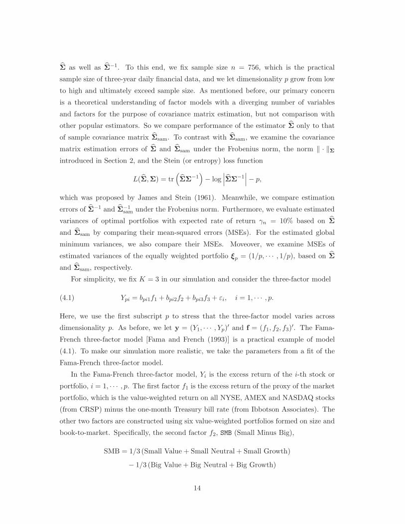
For simplicity, we fix K = 3 in our simulation and consider the three-factor model
(4.1) Ypi = bpi1f1 + bpi2f2 + bpi3f3 + εi, i = 1, · · · , p.
Here, we use the first subscript p to stress that the three-factor model varies across
dimensionality p. As before, we let y = (Y1, · · · , Yp)′ and f = (f1, f2, f3)
′. The Fama-
French three-factor model [Fama and French (1993)] is a practical example of model
(4.1). To make our simulation more realistic, we take the parameters from a fit of the
Fama-French three-factor model.
In the Fama-French three-factor model, Yi is the excess return of the i-th stock or
portfolio, i = 1, · · · , p. The first factor f1 is the excess return of the proxy of the market
portfolio, which is the value-weighted return on all NYSE, AMEX and NASDAQ stocks
(from CRSP) minus the one-month Treasury bill rate (from Ibbotson Associates). The
other two factors are constructed using six value-weighted portfolios formed on size and
book-to-market. Specifically, the second factor f2, SMB (Small Minus Big),
SMB = 1/3 (Small Value + Small Neutral + Small Growth)
− 1/3 (Big Value + Big Neutral + Big Growth)
14
is the average return on the three small portfolios minus the average return on the three
big portfolios, and the third factor f3, HML (High Minus Low),
HML = 1/2 (Small Value + Big Value)
− 1/2 (Small Growth + Big Growth)
is the average return on the two value portfolios minus the average return on the two
growth portfolios. See their website http://mba.tuck.dartmouth.edu/pages/faculty
/ken.french/data_library.html for more details about their three factors and the
data sets of the three factors, risk free interest rates, and returns of many constructed
portfolios.
We first fit three-factor model (4.1) with n = 756 and p = 30 using the three-year
daily data of 30 Industry Portfolios from May 1, 2002 to Aug. 29, 2005, which are avail-
able at the above website. Then, as in (1.4), we get 30 estimated factor loading vectors
b1 = (b11, b12, b13), · · · , b30 = (b30,1, b30,2, b30,3) and 30 estimated standard deviations
σ1, · · · , σ30 of the errors, where bi and σi correspond to the i-th portfolio, i = 1, · · · , 30.The sample average of σ1, · · · , σ30 is 0.66081 with a sample standard deviation 0.3275.
We report in Table 1 the sample means and sample covariance matrices of f and b
denoted by µf, µb and covf, covb, respectively.
Table 1
Sample means and sample covariance matrices of f and b
µf covf
0.023558 1.2507 -0.034999 -0.20419
0.012989 -0.034999 0.31564 -0.0022526
0.020714 -0.20419 -0.0022526 0.19303
µb covb
0.78282 0.029145 0.023873 0.010184
0.51803 0.023873 0.053951 -0.006967
0.41003 0.010184 -0.006967 0.086856
For each simulation, we carry out the following steps:
• We first generate a random sample of f = (f1, f2, f3)′ with size n = 756 from the
trivariate normal distribution N(µf, covf
).
15
• Then, for each dimensionality p increasing from 16 to 1000 with increment 20, we
do the following.
• Generate p factor loading vectors b1, · · · ,bp as a random sample of size p from
the trivariate normal distribution N(µb, covb
).
• Generate p standard deviations σ1, · · · , σp of the errors as a random sample of
size p from a gamma distribution G(α, β) conditional on being bounded below by
a threshold value. The threshold for the standard deviations of errors is required
in accordance with condition (C) in Section 2.1, and it is set to 0.1950 in our
simulation because we find min1≤i≤30 σi = 0.1950. Note that G(α, β) has mean
αβ and standard deviation α1/2β, and its conditional mean and conditional second
moment on falling above 0.1950 can be approximated respectively by
(αβ − 0.1950
2p
)/ (1 − p) and
(αβ2 + α2β2 − 0.19502
2p
)/ (1 − p) ,
where p is the probability of falling below 0.1950 under G(α, β). By matching the
mean 0.66081 and standard deviation 0.3275 for G(α0, β0), we obtain α0 = 4.0713
and β0 = 0.1623. Therefore, following the above approximations, by recursively
matching the conditional mean 0.66081 and conditional second moment 0.32752 +
0.660812 = 0.54393 for G(α, β), we finally get α = 3.3586 and β = 0.1876.
• After getting p standard deviations σ1, · · · , σp of the errors, we generate a random
sample of ε = (ε1, · · · , εp)′ with size n = 756 from the p-variate normal distribution
N(0,diag
(σ2
1, · · · , σ2p
)).
• Then from model (4.1), we get a random sample of y = (Y1, · · · , Yp)′ with size
n = 756.
• Finally, we compute estimated covariance matrices Σ and Σsam, as well as Σ−1
and Σ−1sam, and record the errors in the aforementioned measures. Meanwhile, we
calculate MSEs of estimated variances of the optimal portfolios with γn = 10%
as well as MSEs of estimated global minimum variances based on Σ and Σsam,
respectively. Also, we record MSEs of estimated variances of the equally weighted
portfolio based on Σ and Σsam, respectively.
We repeat the above simulation 500 times and report the mean-square errors as well as
the standard deviations of those errors.
16
0 200 400 600 800 10000
5
10
15
20
25
30
35
40
45
0 200 400 600 800 10000
0.2
0.4
0.6
0.8
1
1.2
1.4
(a) (b)
0 200 400 600 800 10000
0.2
0.4
0.6
0.8
1
1.2
1.4
0 200 400 600 800 10001
2
3
4
5
6
7
8
9
10x 10
−3
(c) (d)
0 50 100 150 200 250 300 350 400
0
20
40
60
80
100
120
140
0 50 100 150 200 250 300 350 4000
0.1
0.2
0.3
0.4
0.5
0.6
0.7
(e) (f)
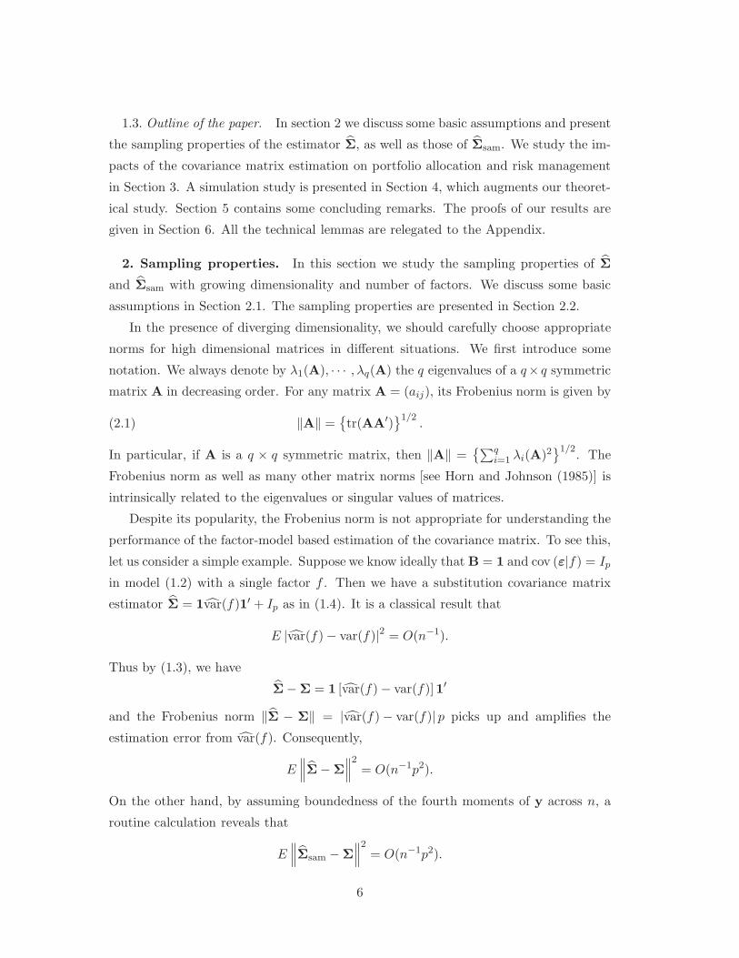
Figure 1: (a), (c) and (e): The averages of errors over 500 simulations for bΣ (solid curve) and bΣsam (dashed
curve) against p under Frobenius norm, norm ‖ · ‖Σ and entropy losses, respectively. (b), (d) and (f): Corre-
sponding standard deviations of errors over 500 simulations for bΣ (solid curve) and bΣsam (dashed curve).
17
0 50 100 150 200 250 300 350 4000
50
100
150
200
250
300
0 50 100 150 200 250 300 350 4000
5
10
15
(a) (b)
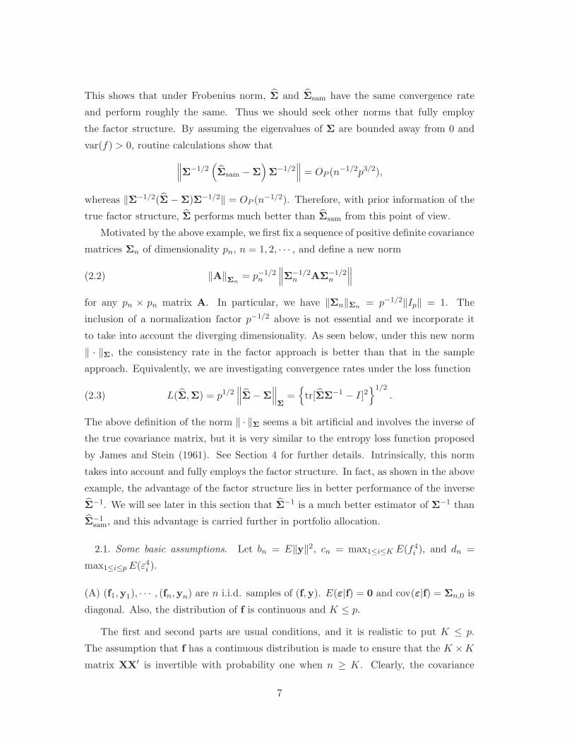
Figure 2: (a) The averages of errors under Frobenius norm over 500 simulations for bΣ−1 (solid curve) and
bΣ−1sam (dashed curve) against p. (b) Corresponding standard deviations of errors under Frobenius norm.
In Figures 1–4, solid curves and dashed curves correspond to Σ and Σsam, respec-
tively. Figure 1 presents the averages and the standard deviations of their estimation
errors under the Frobenius norm, norm ‖ · ‖Σ, and entropy loss against dimensionality
p, respectively. Figure 2 depicts the averages and the standard deviations of estimation
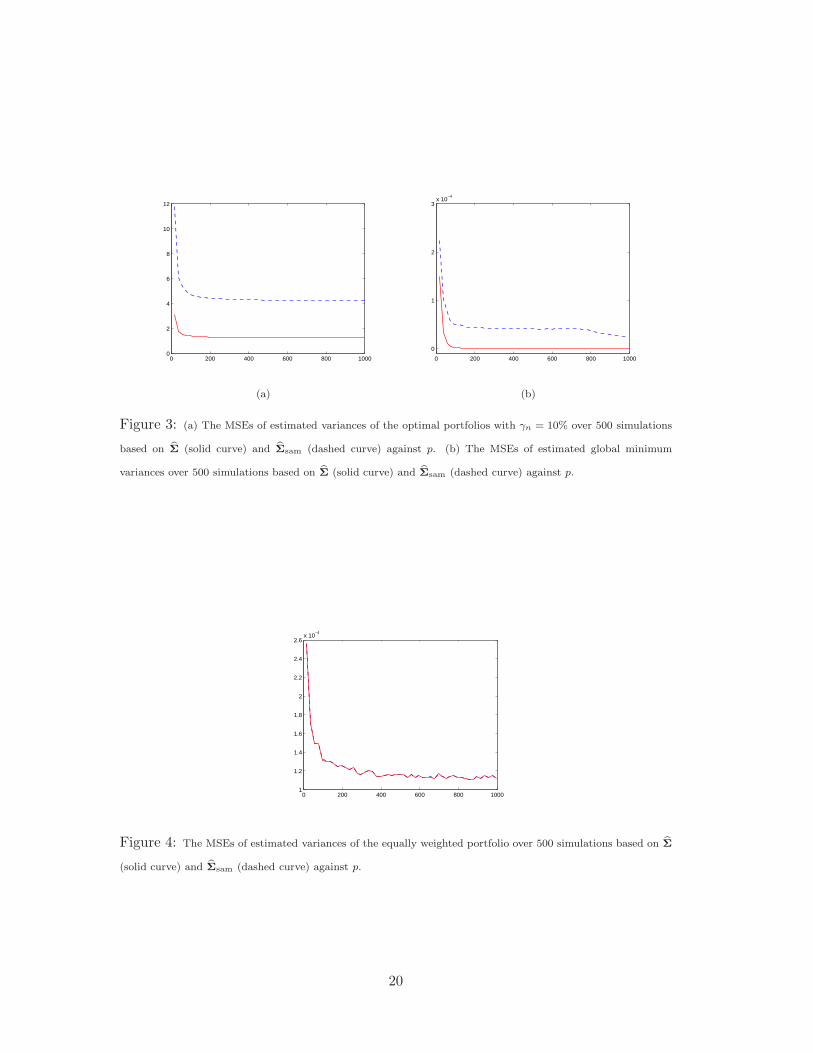
errors of Σ−1 and Σ−1sam under the Frobenius norm against p. We report in Figure 3
MSEs of estimated variances of the optimal portfolios with γn = 10% as well as MSEs
of estimated global minimum variances using Σ and Σsam against p. Figure 4 presents
MSEs of estimated variances of the equally weighted portfolio based on Σ and Σsam
against p.
Recall that both the sample size n and the number of factors K are kept fixed across
p in our simulation. From Figures 1–4, we observe the following:
• By comparing corresponding averages and standard deviations of the errors shown
in Figures 1 and 2, we see that the Monte-Carlo errors are negligible.
• Figure 1(a) shows that under the Frobenius norm, Σ performs roughly the same
as (slightly better than) Σsam, which is consistent with the results in Theorem 1.
Nevertheless, this is a surprise and is against the conventional wisdom.
• Figure 1(c) reveals that under norm ‖ · ‖Σ, Σ performs much better than Σsam,
which is consistent with the results in Theorem 2. In particular, we see that the
estimation errors of Σ under norm ‖ · ‖Σ are roughly at the same level across p.
Recall that sample size n is fixed as 756 here. Thus, this is in line with the root-
18
n-consistency of Σ under norm ‖ · ‖Σ when p = O(n) shown in Theorem 2. Also,
the apparent growth pattern of estimation errors in Σsam with p is in accordance
with its (n/p)1/2-consistency under norm ‖ · ‖Σ shown in Theorem 2.
• Figure 1(e) shows that under entropy loss, Σ significantly outperforms Σsam, which
strongly supports the factor-model based estimator Σ over the sample one Σsam.
We only report the results for p truncated at 400. This is because for larger
p, sample covariance matrices Σsam are nearly singular with a big chance in the
simulation, which results in extremely large entropy losses.
• From Figure 2(a), we see that under the Frobenius norm, the estimator Σ−1
significantly outperforms Σ−1sam, which is in line with the results in Theorem 3.
• Figures 3(a) and 3(b) demonstrate convincingly that Σ outperforms Σsam in port-
folio allocation. These results are in accordance with Theorems 5 and 6. One may
notice that in Figure 3(a), the MSEs are relatively large in magnitude for small
p and then tend to stabilize when p grows large. This is because in our settings
for the simulation, for small p the term ϕnφn − ψ2n is relatively small compared
to ϕnγ2n − 2ψnγn + φn, which results in large variance of the optimal portfolio.
The behavior of the MSEs for large p is essentially due to self-averaging in the
dimensionality. Figures 3(b) can be interpreted in the same way.
• Figure 4 reveals that the factor-model based approach and the sample approach
have almost the same performance in risk management, which is consistent with
Theorem 7. The high-dimensionality behavior is essentially due to self-averaging
as in Figure 3(a).
5. Concluding remarks. This paper investigates the impact of dimensionality on
the estimation of covariance matrices. Two estimators are singled out for studies and
comparisons: the sample covariance matrix and the factor-model based estimate. The
inverse of the covariance matrix takes advantage of the factor structure and hence can
be better estimated in the factor approach. As a result, when the parameters involve the
inverse of the population covariance, substantial gain can be made. On the other hand,
the covariance matrix itself does not take much advantage of the factor structure, and
hence its estimate can not be improved much in the factor approach. This is somewhat
surprising and is against the conventional wisdom.
19
0 200 400 600 800 10000
2
4
6
8
10
12
0 200 400 600 800 1000
0
1
2
3x 10
−4
(a) (b)
Figure 3: (a) The MSEs of estimated variances of the optimal portfolios with γn = 10% over 500 simulations
based on bΣ (solid curve) and bΣsam (dashed curve) against p. (b) The MSEs of estimated global minimum
variances over 500 simulations based on bΣ (solid curve) and bΣsam (dashed curve) against p.
0 200 400 600 800 10001
1.2
1.4
1.6
1.8
2
2.2
2.4
2.6x 10
−4
Figure 4: The MSEs of estimated variances of the equally weighted portfolio over 500 simulations based on bΣ
(solid curve) and bΣsam (dashed curve) against p.
20
Optimal portfolio allocation and minimum variance portfolio involve the inverse of
the covariance matrix. Hence, it is advantageous to employ the factor structure in
portfolio allocation. On the other hand, intrinsically the risk management does not
depend on the covariance structure and hence there is no advantage to appeal to the
factor model in risk management.
Our conclusion is also verified by an extensive simulation study, in which the param-
eters are taken in a neighborhood that is close to the reality. The choice of parameters
relies on a fit to the famous Fama-French three-factor model to the portfolios traded in
the market.
Our studies also reveal that the impact of dimensionality on the estimation of co-
variance matrices is severe. This should be taken into consideration in practical imple-
mentations.
6. Proofs of theorems. In this section, we give rigorous proofs of Theorems 1–7.
Proof of Theorem 1. (1) First, we prove (pK)−1 n1/2-consistency of Σ under
the Frobenius norm. To facilitate the presentation, we introduce here some notation
used throughout the rest of the paper. Let Cn = EX′(XX′)−1,
Dn ={(n− 1)−1
XX′ − [n(n− 1)]−1X11′X′
}− cov(f)
and
Fn = Ip ◦ n−1E (In − H)E′ − Σ0,
where H = X′ (XX′)−1
X is the n×n hat matrix and A1 ◦A2 stands for the Hadamard
product, i.e. the entrywise product, for any q × r matrices A1 and A2. Then we
have B = YX′ (XX′)−1
= B + Cn, cov(f) = (n− 1)−1XX′ − {n (n− 1)}−1
X11′X′ =
cov(f) + Dn, Σ0 = diag(n−1EE
′)
= Σ0 + Fn and
(6.1) Σ = Σ + BDnB′ +[Bcov(f)C′
n + Cncov(f)B′]+ Cncov(f)C′
n + Fn,
This shows that Σ is a four-term perturbation of the population covariance matrix,
and this representation is our key technical tool. By the Cauchy-Schwarz inequality, it
follows from (6.1) that
E‖Σ − Σ‖2 ≤ 4[E tr
{(BDnB
′)2}
+ E tr{[
Bcov(f)C′n + Cncov(f)B′
]2}
+ E tr{[
Cncov(f)C′n
]2}+ E tr
(F2
n
) ].
21
We will examine each of the above four terms on the right hand side separately. For
brevity of notation, we suppress the first subscript n in some situations where the
dependence on n is self-evident.
Before going further, let us bound ‖Bn‖. From assumption (B), we know that
cov(f) ≥ σ1IK , where for any symmetric positive semidefinite matrices A1 and A2,
A1 ≥ A2 means A1 −A2 is positive semidefinite. Thus it follows easily from (1.3) that
σ1BnB′n = Bn (σ1IK)B′
n ≤ Bncov(f)B′n ≤ Σn,
which along with bn = O(p) in assumption (B) shows that ‖Bn‖2 = tr (BnB′n) ≤
tr (Σn) /σ1 ≤ bn
σ1= O(p), i.e.
(6.2) ‖Bn‖ = O(p1/2).
Clearly, ‖B′nBn‖ = ‖BnB
′n‖, and by (A.1) in Lemma 1 and (6.2) we have
(6.3) ‖B′nBn‖ = ‖BnB
′n‖ ≤ ‖Bn‖‖B′
n‖ = ‖Bn‖2 = O(p).
This fact is a key observation that will be used very often, and as shown above, it is
entailed only by assumptions (A) and (B), which are valid throughout the paper.
Now we consider the first term, say E tr{(BDnB′)
2}. From cn = O(1) in assumption
(B), we see that the fourth moments of f are bounded across n, thus a routine calculation
reveals that
(6.4) E(‖Dn‖2
)= O(n−1K2),
which is an important fact that will be used very often and also helps study the inverse
cov(f)−1 by keeping in mind that K → ∞. By (A.2) in Lemma 1, (6.3), and (6.4), we
have
(6.5) E tr[(
BDnB′)2] ≤
∥∥B′B∥∥2E(‖Dn‖2
)= O(n−1(pK)2).
The remaining three terms are taken care of by Lemmas 2 and 3. Therefore, in view
of (6.3), combining (6.5) with (A.5)–(A.7) in Lemmas 2 and 3 gives
E∥∥∥Σ− Σ
∥∥∥2
= O(n−1(pK)2).
In particular, this implies that∥∥∥Σ − Σ
∥∥∥ = OP (n−1/2pK), which proves (pK)−1 n1/2-
consistency of the covariance matrix estimator Σ under Frobenius norm.
22
(2) Then, we show that Σsam is (pK)−1 n1/2-consistent under the Frobenius norm.
By (1.3) and (1.5), we have
Σsam = Σ + BDnB′ + Gn + (n− 1)−1 {
BXE′ + EX′B}
(6.6)
− [n (n− 1)]−1 {BX11′E′ + E11′X′B′
},
where Gn ={
(n− 1)−1EE′ − [n(n− 1)]−1
E11′E′}−Σ0. This shows that Σsam is also
a four-term perturbation of the population covariance matrix. By the Cauchy-Schwarz
inequality, it follows from (6.6) that
E∥∥∥Σsam − Σ
∥∥∥2≤ 4
[E∥∥BDnB
′∥∥2
+ E ‖Gn‖2 + 2 (n− 1)−2E∥∥BXE′
∥∥2
+ 2 [n (n− 1)]−2E∥∥BX11′E′
∥∥2].
As in part (1), we will examine each of the above four terms on the right hand side
separately. The first term E ‖BDnB′‖2
has been bounded in (6.5). Using the same
argument as in Lemma 6, we can show that E ‖Gn‖2 = O(n−1p2). In view of (6.3), it
is shown that
E∥∥BXE′
∥∥2= O(np2K)
in the proof of Lemma 2. Using the same argument as in Lemma 2 to boundE ‖BX11′HE′‖2,
we can easily get
E∥∥BX11′E′
∥∥2= O(n3p2K),
which along with (6.5) and the above results yields
E∥∥∥Σsam − Σ
∥∥∥2
= O(n−1(pK)2).
This proves (pK)−1 n1/2-consistency of Σsam under the Frobenius norm.
(3) Finally, we prove the uniform weak convergence of eigenvalues. It follows from
Corollary 6.3.8 of Horn and Johnson (1985) that
max1≤k≤p
∣∣∣λk(Σn) − λk(Σn)∣∣∣ ≤
{p∑
k=1
[λk(Σn) − λk(Σn)
]2}1/2
≤∥∥∥Σn − Σn
∥∥∥ .
Therefore, the uniform weak convergence of the eigenvalues of the Σn’s follows imme-
diately from the (pK)−1 n1/2-consistency of Σ under the Frobenius norm shown in part
(1). Similarly, by the (pK)−1 n1/2-consistency of Σsam under the Frobenius norm shown
in part (2), the same conclusion holds for Σsam. �
23
Proof of Theorem 2. (1) First, we show that Σ is nβ/2-consistent under norm
‖ · ‖Σ. The main idea of the proof is similar to that of Theorem 1, but the proof is more
tricky and involved here since the norm ‖ · ‖Σ involves the inverse of the covariance
matrix Σ. By the Cauchy-Schwarz inequality, it follows from (6.1) that
E∥∥∥Σ− Σ
∥∥∥2
Σ
≤ 4[E∥∥BDnB
′∥∥2
Σ+ E
∥∥Bcov(f)C′n + Cncov(f)B′
∥∥2
Σ
+ E∥∥Cncov(f)C′
n
∥∥2
Σ} + E ‖Fn‖2
Σ
].
As in the proof of Theorem 1, we will study each of the above four terms on the right
hand side separately.
Before going further, let us bound∥∥B′Σ−1B
∥∥. From (1.3), we know that Σ =
Σ0+Bcov(f)B′, which along with the Sherman-Morrison-Woodbury formula shows that
(6.7) Σ−1 = Σ−10 − Σ−1
0 B[cov(f)−1 + B′Σ−1
0 B]−1
B′Σ−10 .
Thus it follows that
B′Σ−1B = B′Σ−10 B− B′Σ−1
0 B[cov(f)−1 + B′Σ−1
0 B]−1
B′Σ−10 B
= B′Σ−10 B
[cov(f)−1 + B′Σ−1
0 B]−1
cov(f)−1
= cov(f)−1 − cov(f)−1[cov(f)−1 + B′Σ−1
0 B]−1
cov(f)−1,
which implies that
∥∥B′Σ−1B∥∥ ≤
∥∥cov(f)−1∥∥+
∥∥∥cov(f)−1[cov(f)−1 + B′Σ−1
0 B]−1
cov(f)−1∥∥∥ .
Note that cov(f)−1 is symmetric positive definite and B′Σ−10 B is symmetric positive
semidefinite. Thus, cov(f)−1+B′Σ−10 B ≥ cov(f)−1, which in turn implies that
[cov(f)−1 + B′Σ−1
0 B]−1 ≤
cov(f) and
cov(f)−1[cov(f)−1 + B′Σ−1
0 B]−1
cov(f)−1 ≤ cov(f)−1cov(f)cov(f)−1 = cov(f)−1.
In particular, this entails that
∥∥∥cov(f)−1[cov(f)−1 + B′Σ−1
0 B]−1
cov(f)−1∥∥∥ ≤
∥∥cov(f)−1∥∥ ,
so now the problem of bounding∥∥B′Σ−1B
∥∥ reduces to bounding∥∥cov(f)−1
∥∥. By as-
sumption (B), λK(cov(f)) ≥ σ1 for some constant σ1 > 0. Thus the largest eigenvalues
of cov(f)−1 are bounded across n, which easily implies that∥∥cov(f)−1
∥∥ = O(K1/2). This
together with the above results shows that
(6.8)∥∥B′Σ−1B
∥∥ = O(K1/2).
24
Now we are ready to examine the first term, say E ‖BDnB′‖2
Σ. By (A.1) in Lemma
1, we have
∥∥BDnB′∥∥2
Σ= p−1tr
[(DnB
′Σ−1B)2] ≤ p−1 ‖Dn‖2
∥∥B′Σ−1B∥∥2.
Therefore, it follows from (6.4) and (6.8) that
(6.9) E∥∥BDnB
′∥∥2
Σ= O(n−1p−1K3).
Then, we consider the second term E ‖Bcov(f)C′n + Cncov(f)B′‖2
Σ. Note that
E∥∥Bcov(f)C′
n + Cncov(f)B′∥∥2
Σ≤ 2
[E∥∥Bcov(f)C′
n
∥∥2
Σ+ E
∥∥Cncov(f)B′∥∥2
Σ
](6.10)
= 4 E∥∥Bcov(f)C′
n
∥∥2
Σ≤ 8[(n− 1)−2E
∥∥BXX′C′n
∥∥2
Σ
+ n−2 (n− 1)−2E∥∥BX11′X′C′
n
∥∥2
Σ
]
= 8 (n− 1)−2 L1 + 8n−2 (n− 1)−2 L2.
Since E(ε|f) = 0, conditioning on X gives
L1 = p−1E tr[XE
(E′Σ−1E|X
)X′B′Σ−1B
]
= p−1E tr[X tr
(Σ−1Σ0
)In X′B′Σ−1B
]
≤ p−1tr(Σ−1Σ0
)E(‖XX′‖
) ∥∥B′Σ−1B∥∥ .
In the proof of Lemma 2, it is shown that E(‖XX′‖2
)= O(n2K2), which implies that
E(‖XX′‖
)≤[E(‖XX′‖2
)]1/2= O(nK).
By (1.3) and assumptions (B) and (C), we can easily get
tr(Σ−1Σ0
)≤ tr
(Σ−1
)O(1) = O(p),
which along with (6.8) and the above results shows that
L1 = O(nK3/2).
Similarly, by conditioning on X we have
L2 = p−1E tr[X11′HE
(E′Σ−1E|X
)H11′X′B′Σ−1B
]
= p−1E tr[X11′H tr
(Σ−1Σ0
)In H11′X′B′Σ−1B
].
25
Then, applying (A.1)–(A.3) in Lemma 1 gives
L2 ≤ p−1tr(Σ−1Σ0
)E∥∥X11′H11′X′
∥∥∥∥B′Σ−1B∥∥
≤ p−1tr(Σ−1Σ0
)E ‖H‖
∥∥X′X∥∥ ∥∥11′11′
∥∥ ∥∥B′Σ−1B∥∥
= n2p−1K1/2tr(Σ−1Σ0
)E∥∥X′X
∥∥ ∥∥B′Σ−1B∥∥ ,
which together with the above results shows that
L2 = O(n3K2).
Thus, in view of (6.10) we have
(6.11) E∥∥Bcov(f)C′
n + Cncov(f)B′∥∥2
Σ= O(n−1K2).
The third and fourth terms are examined in Lemmas 4 and 5, respectively. Since
K ≤ p by assumption (A), combining (6.9) and (6.11) with (A.8) and (A.11) in Lemmas
4 and 5 results in
E∥∥∥Σ − Σ
∥∥∥2
Σ
= O(n−1K2) +O(n−2pK).
In particular, when K = O(nα1) and p = O(nα) for some 0 ≤ α1 < 1/2 and 0 ≤ α <
2 − α1, we have ∥∥∥Σ − Σ
∥∥∥Σ
= OP (n−β/2)
with β = min (1 − 2α1, 2 − α− α1), which proves nβ/2-consistency of covariance matrix
estimator Σ under norm ‖ · ‖Σ.
(2) Then, we prove the nβ1/2-consistency of Σsam under norm ‖·‖Σ. By the Cauchy-
Schwarz inequality, it follows from (6.6) that
E∥∥∥Σsam − Σ
∥∥∥2
Σ
≤ 4[E∥∥BDnB
′∥∥2
Σ+ E ‖Gn‖2
Σ+ 2 (n− 1)−2E
∥∥BXE′∥∥2
Σ
+ 2 [n (n− 1)]−2E∥∥BX11′E′
∥∥2
Σ
].
As in part (1), we will examine each of the above four terms on the right hand side
separately. The first term E ‖BDnB′‖2
Σhas been bounded in (6.9), and the second
term E ‖Gn‖2Σ
is considered in Lemma 6. The third term E ‖BXE′‖2Σ
is exactly L1 in
part (1) above. Using the same argument that was used in part (1) to prove L2, we can
easily get
E∥∥BX11′E′
∥∥2
Σ= O(n3K3/2).
Thus, by (6.9) and (A.12) in Lemma 6 along with the above results, we have
E∥∥∥Σsam − Σ
∥∥∥2
Σ
= O(n−1p−1K3) +O(n−1p) +O(n−1K3/2).
26
In particular, when K = O(nα1) and p = O(nα) for some 0 ≤ α < 1 and 0 ≤ α1 <
(1 + α) /3, we have ∥∥∥Σsam − Σ
∥∥∥Σ
= OP (n−β1/2)
with β1 = 1 − max(α, 3α1/2, 3α1 − α), which shows nβ1/2-consistency of Σsam under
norm ‖ · ‖Σ. �
Proof of Theorem 3. (1) First, we prove the weak convergence of Σ−1sam under
the Frobenius norm. Note that Σsam involves sample covariance matrix estimation of
Σ0, so the technique in part (2) below does not help. In general, the only available way
is as follows. We define Qn = Σsam −Σn. It is a basic fact in matrix theory that
(6.12)∥∥∥Σ−1
sam − Σ−1n
∥∥∥ ≤∥∥Σ−1
n
∥∥∥∥Σ−1
n Qn
∥∥1 −
∥∥Σ−1n Qn
∥∥ ≤∥∥Σ−1
n
∥∥2 ‖Qn‖1 −
∥∥Σ−1n
∥∥ ‖Qn‖
whenever∥∥Σ−1
n
∥∥ ‖Qn‖ < 1. From Theorem 1, we know that
‖Qn‖ = OP (n−1/2pK).
By (A.9), we have∥∥Σ−1
n
∥∥ = O(p1/2). Since pK1/2 = o((n/ log n)1/4) we see that
∥∥Σ−1n
∥∥ ‖Qn‖P−→ 0 and
√np−4K−2/ log n
∥∥Σ−1n
∥∥2 ‖Qn‖P−→ 0.
It follows easily that
√np−4K−2/ log n
∥∥Σ−1n
∥∥2 ‖Qn‖1 −
∥∥Σ−1n
∥∥ ‖Qn‖P−→ 0,
which along with (6.12) shows that
√np−4K−2/ log n
∥∥∥Σ−1sam − Σ−1
n
∥∥∥ P−→ 0 as n→ ∞.
(2) Then, we show the weak convergence of Σ−1 under the Frobenius norm. The
basic idea is to examine the estimation error for each term of Σ−1, which has an explicit
form thanks to the factor structure. From (1.4), we know that Σ = Bcov(f)B′+ Σ0,
which along with the Sherman-Morrison-Woodbury formula shows that
(6.13) Σ−1 = Σ−10 − Σ−1
0 B[cov(f)−1 + B
′Σ−1
0 B]−1
B′Σ−1
0 .
27
Thus by (6.7), we have
∥∥∥Σ−1 −Σ−1∥∥∥ ≤
∥∥∥Σ−10 −Σ−1
0
∥∥∥+
∥∥∥∥(Σ−1
0 − Σ−10
)B[cov(f)−1 + B
′Σ−1
0 B]−1
B′Σ−1
0
∥∥∥∥
(6.14)
+
∥∥∥∥Σ−10 B
[cov(f)−1 + B
′Σ−1
0 B]−1
B′(Σ−1
0 − Σ−10
)∥∥∥∥
+
∥∥∥∥Σ−10
(B− B
) [cov(f)−1 + B
′Σ−1
0 B]−1
B′Σ−1
0
∥∥∥∥
+
∥∥∥∥Σ−10 B
[cov(f)−1 + B
′Σ−1
0 B]−1 (
B′ − B′
)Σ−1
0
∥∥∥∥
+
∥∥∥∥Σ−10 B
{[cov(f)−1 + B
′Σ−1
0 B]−1
−[cov(f)−1 + B′Σ−1
0 B]−1}
B′Σ−10
∥∥∥∥
= K1 + K2 + K3 + K4 + K5 + K6.
To study∥∥∥Σ−1 − Σ−1
∥∥∥, we need to examine each of the above six terms K1, · · · ,K6
separately, so it would be lengthy work to check all the details here. Therefore, we only
sketch the idea of the proof and leave the details to the reader.
From assumption (C), we know that the diagonal entries of Σ0 are bounded away
from 0. Note that Σ0 and Σ0 are both diagonal, and thus, by the same argument as in
Lemma 5, we can easily show that
(6.15) K1 =∥∥∥Σ−1
0 − Σ−10
∥∥∥ = OP (n−1/2p1/2) +OP (n−1pK1/2) = OP (n−1/2p1/2),
since pK1/2 = o((n/ log n)1/2). Now we consider the second term K2. By (A.1) in
Lemma 1, we have
K2 ≤∥∥∥(Σ−1
0 − Σ−10
)Σ
1/20
∥∥∥∥∥∥∥Σ
−1/20 B
[cov(f)−1 + B
′Σ−1
0 B]−1
B′Σ
−1/20
∥∥∥∥∥∥∥Σ−1/2
0
∥∥∥
= L1L2
∥∥∥Σ−1/20
∥∥∥ ,
and we will examine each of the above two terms L1 and L2, as well as∥∥∥Σ−1/2
0
∥∥∥. Since
Σ0 and Σ0 are diagonal, a similar argument to that bounding K1 above applies to show
that ∥∥∥Σ−1/20
∥∥∥ = OP (p1/2) and L1 = OP (n−1/2p1/2).
Clearly, Σ−1/20 B
[cov(f)−1 + B
′Σ−1
0 B]−1
B′Σ
−1/20 is symmetric positive semidefinite with
rank at most K and Σ1/20 Σ−1Σ
1/20 ≥ 0. Thus it follows from (6.13) that
Σ−1/20 B
[cov(f)−1 + B
′Σ−1
0 B]−1
B′Σ
−1/20 = Ip − Σ
1/20 Σ−1Σ
1/20 ≤ Ip,
28
which implies that Σ−1/20 B
[cov(f)−1 + B
′Σ−1
0 B]−1
B′Σ
−1/20 has at most K positive
eigenvalues and all of them are bounded by one. This shows that L2 ≤ K1/2, which
along with the above results gives
(6.16) K2 = OP (n−1/2pK1/2).
Similarly, we can also show that
(6.17) K3 = OP (n−1/2pK1/2).
Then we consider terms K4 and K5. Clearly, cov(f)−1 + B′Σ−1
0 B ≥ cov(f)−1, which
in turn entails that[cov(f)−1 + B
′Σ−1
0 B]−1
≤ cov(f) and
∥∥∥∥[cov(f)−1 + B
′Σ−1
0 B]−1∥∥∥∥ ≤ ‖cov(f)‖ .
It is easy to show that ‖cov(f)‖ = OP (K). Thus we have
K4 ≤∥∥∥Σ−1
0
(B− B
)∥∥∥∥∥∥∥[cov(f)−1 + B
′Σ−1
0 B]−1∥∥∥∥∥∥∥B′
Σ−10
∥∥∥(6.18)
= OP (n−1p1/2)OP (K)OP (p1/2) = OP (n−1/2pK)
and
K5 ≤∥∥Σ−1
0 B∥∥∥∥∥∥[cov(f)−1 + B
′Σ−1
0 B]−1∥∥∥∥∥∥∥(B
′ − B′)Σ−1
0
∥∥∥(6.19)
= OP (p1/2)OP (K)OP (n−1p1/2K) = OP (n−1/2pK).
Finally, by the same argument as in part (1) above, we can show that
∥∥∥∥[cov(f)−1 + B
′Σ−1
0 B]−1
−[cov(f)−1 + B′Σ−1
0 B]−1∥∥∥∥ = oP ((n/ log n)−1/2K2).
Thus by (A.2) in Lemma 1, we have
K6 ≤∥∥∥∥[cov(f)−1 + B
′Σ−1
0 B]−1
−[cov(f)−1 + B′Σ−1
0 B]−1∥∥∥∥∥∥B′Σ−2
0 B∥∥(6.20)
= oP ((n/ log n)−1/2K2)O(p) = oP ((n/ log n)−1/2 pK2).
Therefore, it follows from (6.14)–(6.20) that
√np−2K−4/ log n
∥∥∥Σ−1n − Σ−1
n
∥∥∥ P−→ 0 as n→ ∞,
which completes the proof. �
29
Proof of Theorem 4. We aim at establishing asymptotic normality of the K×Kmatrix
√np−2B′
(Σ − Σ
)B, and only here are the K factors f1, · · · , fK assumed fixed
across n. The basic idea is to use its four-term decomposition below and to show that
the first term has asymptotic normality by the classical central limit theorem, while the
remaining three terms are all negligible, say oP (1), which along with Slutsky’s theorem
leads to the desired conclusion. In view of (6.1), we have
√np−2B′
(Σ − Σ
)B =
√np−2B′BDnB
′B +√np−2B′
{Bcov(f)C′
n + Cncov(f)B′}B
+√np−2B′Cncov(f)C′
nB +√np−2B′FnB
= A1 + A2 + A3 + A4.(6.21)
We will study each of the above four terms A1, · · · ,A4 separately.
First, we consider the term A1. Define
Hn =n
n− 1
(n−1
n∑
i=1
fi − Ef
)(n−1
n∑
i=1
f′i − Ef′
).
Then we have
(6.22) cov(f) = (n− 1)−1n∑
i=1
(fi − Ef)(f′i − Ef′
)−Hn.
By the classical central limit theorem, we know that
√n
(n−1
n∑
i=1
fi − Ef
)D−→ N (0, cov(f)) .
It follows from the law of large numbers that n−1∑n
i=1 fi−EfP−→ 0. Thus, by Slutsky’s
theorem we have√nHn
D−→ 0, which in turn implies that
√nHn
P−→ 0;
that is, Hn = oP (n−1/2). So in view of (6.22), we have
(6.23) cov(f) = n−1n∑
i=1
(fi − Ef)(f′i − Ef′
)+ oP (n−1/2).
Therefore, it follows easily from p−1B′nBn → A and (6.23) that
(6.24) A1 = A
{n−1/2
n∑
i=1
[(fi −Ef)
(f′i − Ef′
)− cov(f)
]}
A + oP (1).
30
We define
n−1/2n∑
i=1
[(fi − Ef)
(f′i − Ef′
)− cov(f)
]= Un = (uij)K×K .
By the classical central limit theorem, we know that [see, e.g. Muirhead (1982)]
(6.25) vech (Un)D−→ N (0,H) ,
where H is determined in an obvious way by
cov (uij, ukl) = κijkl + κikκjl + κilκjk,
with κi1···ir the central moment E [(fi1 −Efi1) · · · (fir − Efir)] of f = (f1, · · · , fK)′. It
follows easily from (6.24) and (6.25) that
(6.26) vech (A1)D−→ N (0, G) ,
where G = PD (A⊗ A)DHD′ (A⊗ A)P ′D, D is the duplication matrix of order K, and
PD = (D′D)−1D′.
Then, we examine the second term A2. From p−1B′nBn → A, we know that
(6.27)∥∥B′
nBn
∥∥ =∥∥BnB
′n
∥∥ = O(p),
which is in line with (6.3). It follows that
‖A2‖ ≤ 2∥∥√np−2B′Bcov(f)C′
nB∥∥ ≤ 2n1/2p−2
∥∥B′B∥∥ ∥∥cov(f)C′
nB∥∥(6.28)
≤ 2n1/2p−2∥∥B′B
∥∥{
(n− 1)−1∥∥XE′B
∥∥+ n−1 (n− 1)−1∥∥X11′HE′B
∥∥}
= O(n−1/2p−1)∥∥XE′B
∥∥+O(n−3/2p−1)∥∥X11′HE′B
∥∥ .
Since E(ε|f) = 0 and Σ0 is diagonal, conditioning on X gives
E∥∥XE′B
∥∥2= E tr
[XE
(E′BB′E|X
)X′]
= E tr[X tr
(BB′Σ0
)In X′
]
= tr(BB′Σ0
)E ‖X‖2 = O(p)O(n) = O(np).
Similarly, by conditioning on X we have
E∥∥X11′HE′B
∥∥2= E tr
[X11′HE
(E′BB′E′|X
)H11′X′
]
= E tr[X11′H tr
(BB′Σ0
)In H11′X′
]
31
and then applying (A.2) and (A.3) in Lemma 1 yields
E∥∥X11′Hε′B
∥∥2 ≤ tr(BB′Σ0
)E{∥∥X′X
∥∥ ∥∥11′11′∥∥ ‖H‖
}
≤ O(p)n2K1/2{E(‖X′X‖2
)}1/2= O(n3p).
It follows that ‖XE′B‖ = OP (n1/2p1/2) and ‖X11′HE′B‖ = OP (n3/2p1/2), which to-
gether with (6.28) shows that
(6.29) A2 = oP (1);
that is, A2 is a negligible term.
Finally, the third and fourth terms A3 and A4 can also be shown to be negligible by
invoking Lemma 3. By (6.27) and (A.6) and (A.7) in Lemma 3, we have
E∥∥B′Cncov(f)C′
nB∥∥2 ≤
∥∥BB′∥∥2E∥∥Cncov(f)C′
n
∥∥2
= O(p2)O(n−2p2) = O(n−2p4)
and
E∥∥B′FnB
∥∥2 ≤∥∥BB′
∥∥2E ‖Fn‖2 = O(p2)O(n−1p) = O(n−1p3).
It follows that ‖B′Cncov(f)C′nB‖ = OP (n−1p2) and ‖B′FnB‖ = OP (n−1/2p3/2), which
implies that
(6.30) A3 = oP (1) and A4 = oP (1).
Therefore, in view of (6.26), (6.29), and (6.30), applying Slutsky’s theorem gives
√n vech
[p−2B′
n
(Σn − Σn
)Bn
]D−→ N (0, G) ,
which proves the asymptotic normality of covariance matrix estimator Σ. �
Proof of Theorem 5. (1) First, we prove the weak convergence of the estimated
global minimum variance based on Σ. From Theorem 3, we know that
√np−2K−4/ log n
∥∥∥Σ−1 −Σ−1∥∥∥ P−→ 0.
Note that
|ϕn − ϕn| =∣∣∣1′(Σ−1 − Σ−1
)1
∣∣∣ =∣∣∣tr[(
Σ−1 − Σ−1)11′]∣∣∣
≤∥∥∥Σ−1 −Σ−1
∥∥∥∥∥11′
∥∥ = p∥∥∥Σ−1 − Σ−1
∥∥∥ .
32
Thus we have √n (pK)−4 / log n |ϕn − ϕn| P−→ 0.
Since all the ϕn’s are bounded away from zero, it follows easily that√n (pK)−4 / log n
∣∣∣ξ′ngΣnξng − ξ′ngΣnξng
∣∣∣ =
√n (pK)−4 / log n
∣∣ϕ−1n − ϕ−1
n
∣∣ P−→ 0.
(2) Then, we prove the conclusion for Σsam. From Theorem 3, we know that
√np−4K−2/ log n
∥∥∥Σ−1sam − Σ−1
∥∥∥ P−→ 0.
Therefore, the above argument in part (1) applies to show that
√np−6K−2/ log n
∣∣∣ξ′ngΣsamξng − ξ′ngΣnξng
∣∣∣ =√np−6K−2/ log n
∣∣ϕ−1n − ϕ−1
n
∣∣ P−→ 0. �
Proof of Theorem 6. (1) First, we prove the weak convergence of the estimated
variance of the optimal portfolio based on Σ. From Theorem 3, we know that
(6.31)√np−2K−4/ log n
∥∥∥Σ−1 −Σ−1∥∥∥ P−→ 0,
and from part (1) in the proof of Theorem 5, we see that
(6.32)
√n (pK)−4 / log n |ϕn − ϕn| P−→ 0.
Now we show the same rate for∣∣∣ψn − ψn
∣∣∣, say
(6.33)
√n (pK)−4 / log n
∣∣∣ψn − ψn
∣∣∣ P−→ 0.
By bn = O(p) in assumption (B), a routine calculation yields ‖µn‖ = O(p1/2) and
E ‖µn − µn‖2 = O(n−1p), and thus
‖µn − µn‖ = OP (n−1/2p1/2).
It follows that∣∣∣ψn − ψn
∣∣∣ ≤∣∣∣1′(Σ−1 − Σ−1
)µ
∣∣∣+∣∣1′Σ−1 (µ − µ)
∣∣ ≤∥∥1′∥∥∥∥∥Σ−1 −Σ−1
∥∥∥
· (‖µ‖ + ‖µ − µ‖) +∥∥1′∥∥ ∥∥Σ−1
∥∥ ‖µ − µ‖ .
Then we have∣∣∣ψn − ψn
∣∣∣ ≤ p1/2∥∥∥Σ−1 − Σ−1
∥∥∥[O(p1/2) +OP (n−1/2p1/2)
]
+ p1/2O(p1/2)OP (n−1/2p1/2)
=∥∥∥Σ−1 − Σ−1
∥∥∥O(p) +OP (n−1/2p3/2) =∥∥∥Σ−1 − Σ−1
∥∥∥O(p),
33
which together with (6.31) proves (6.32). Similarly, we can also show that
(6.34)
√n (pK)−4 / log n
∣∣∣φn − φn
∣∣∣ P−→ 0.
Since ϕnφn − ψ2n are bounded away from zero and ϕn/(ϕnφn − ψ2
n), ψn/(ϕnφn − ψ2n),
φn/(ϕnφn − ψ2n), γn are bounded, the conclusion follows from (3.3) and (6.32)–(6.34).
(2) Now we prove the conclusion for Σsam. From Theorem 3, we know that
√np−4K−2/ log n
∥∥∥Σ−1sam − Σ−1
∥∥∥ P−→ 0,
and from part (2) in the proof of Theorem 5, we see that
√np−6K−2/ log n |ϕn − ϕn| P−→ 0.
Since bn = O(p) by assumption (B), a routine calculation shows that
‖µsam − µn‖ = OP (n−1/2p1/2),
where µsam is the sample mean of µn. Therefore, the argument in part (1) above applies
to show that
√np−6K−2/ log n
∣∣∣ξ′nΣsamξn − ξ′nΣnξn
∣∣∣ P−→ 0 as n→ ∞. �
Proof of Theorem 7. Since ξn = O(1)1, the conclusion follows easily from
consistency results of Σ and Σsam under the Frobenius norm in Theorem 1. In particular,
when the portfolios ξn = (ξ1, · · · , ξp)′ have no short positions, we have
‖ξn‖ =√ξ21 + · · · + ξ2p ≤
√ξ1 + · · · + ξp = 1.
It therefore follows easily that√n (pK)−2 / log n
∣∣∣ξ′nΣnξn − ξ′nΣnξn
∣∣∣ P−→ 0 as n→ ∞
and √n (pK)−2 / log n
∣∣∣ξ′nΣsamξn − ξ′nΣnξn
∣∣∣ P−→ 0 as n→ ∞. �
APPENDIX
Throughout the paper, we denote by H the n× n hat matrix X′ (XX′)−1
X, which
is symmetric and positive semidefinite with probability one by assumption (A).
Lemma 1 (Basic facts).
34
(i) For any q × r matrix A1 and r × q matrix A2, we have


![Robust Shrinkage Estimation of High-dimensional Covariance … · 2010-09-28 · robust covariance estimator [Tyler(1987)], which is distribution-free within the family of elliptical](https://static.documents.pub/doc/80x56/5ed6e20bdf0eda5e752ae517/robust-shrinkage-estimation-of-high-dimensional-covariance-2010-09-28-robust-covariance.jpg)


