High Precision Symplectic Numerical Relative OrbitPropagation

E. Imre & P. L. Palmer

Surrey Space Centre,University of Surrey,Guildford, GU2 7XH,

UK

Abstract

This paper presents a numerical method to propagate relative orbits. It can handleup to an arbitrary number of zonal and tesseral geopotential terms and can be extendedto accommodate the effects of atmospheric drag as well as other perturbations. Thismethod relies on defining a ‘relative Hamiltonian,’ which describes both the absoluteand the relative motion of two satellites. Exploiting the separability of the solution,the Keplerian motion is described via analytical means whereas the effects of higherorder terms are handled via a symplectic numerical integration scheme. The derivationand the numerical integration are designed to conserve the constants of the motion,resulting in better long term accuracy.

When used within a relative orbit estimator, such a high precision relative orbitpropagator should reduce the frequency of the required sensor input dramatically fora given estimation accuracy.

We present results for a broad range of scenarios with large separations and showthat sub-metre accuracy is possible over five days of propagation with a geopotentialmodel containing 36 terms in tesseral and zonal harmonics. These results are validfor eccentricities reaching 0.5. Furthermore, the relative propagation scheme is signifi-cantly faster than differencing two absolute orbit propagations.

1

1 Introduction

The mathematical models to compute the relative motion of two satellites essentially com-

prise integration of the known forces, via either analytical or numerical means. The former

gives a good insight into the dynamics of the problem, but it is difficult to include the effects

of the higher order geopotentials and certain simplifications need to be made, with penalties

in accuracy. On the other hand, the numerical integration schemes, while not giving as much

information regarding the nature of the motion, are simpler to implement, even with high

order geopotentials, lunisolar effects and drag. Therefore, they yield much better accuracy

than their analytical counterparts in real life applications.

For relative navigation, the usual approach has been to make use of simple analytical

models. Perhaps the most well-known is the Clohessy-Wiltshire (CW) [1] or Hill’s Equations

[2], which is simply the linearised Keplerian relative motion for near circular orbits, employed

successfully for short-term rendezvous type missions.

A significant number of researchers derived various methods to extend this near-circular

Keplerian solution to include the effects of J2 [3, 4, 5, 6, 7, 8], eccentricity [9, 10, 11, 12, 13]

and drag [14]. There were also some attempts at incorporating higher order geopotentials

into the solution but with eccentricity limitations [15, 16, 17, 18]. Karlgaard and Lutze [19]

derived second-order, rather than linear, Keplerian relative motion equations for formations

on circular orbits.

Recently Melton [20] and Alfriend and Han [21] published evaluations of different ap-

proaches for the analytical modelling of the relative motion, the latter via an error index

they have defined. They show that, not surprisingly, J2 inclusive nonlinear models provide

much better long term accuracy than their Keplerian-only counterparts and CW equations

have difficulty handling even very small (10−3 level) eccentricities. This underlines the im-

portance of employing better geopotential models.

The literature on numerical relative orbit propagation, on the other hand, is virtually

non-existent. One interesting exception is Encke’s Method [22], which is originally used for

2

numerical integration of perturbed orbits, where the perturbations to the Keplerian orbit

are integrated numerically.

There are a few common threads that can be identified within the existing literature

in the relative motion field. The most important is the universal reliance on analytical

methods. However, analytical methods become extremely complicated when perturbations

to the Keplerian potential such as J2 are integrated into the model. This makes it practically

impossible to employ high fidelity models of the geopotential or drag.

Secondly, virtually all of the methods use a rotating and accelerating local coordinate

frame. While this approach makes analysis and visualisation of the motion rather straight-

forward, it hampers the addition of perturbations as they are usually defined in inertial or

rotating Earth centred frames. This is one of the crucial reasons as to why the addition of

the simple J2 perturbation term greatly complicates the equations.

Perhaps more importantly, these methods do not explicitly address the issue of constants

of the motion. For the motion of a satellite under an axisymmetric potential, the energy

and the z component of the angular momentum (in the Earth Centred Inertial frame) are

both conserved. The same is true for the case of the two satellites; the ‘relative energy’ and

the ‘relative angular momentum in z direction’ should also be conserved. If these quantities

are not conserved, the relative orbit will get distorted over time. For example, any deviation

from the relative energy will manifest itself as an alongtrack drift. In fact, a significant part

of the relative positioning errors observed in the literature are down to the errors in relative

energy, as the forces are integrated in a way that does conserve some constants, though they

do not exactly correspond to the real constants of the motion. Therefore, imposing these

conservation laws should increase the accuracy and duration of the validity of the relative

orbit propagator. Unfortunately, most of the literature provides results for fairly simple cases

and for very short durations (usually from about a single orbit to about a day), making it

very difficult to assess and compare the accuracy of their solutions.

In summary, analytical models for the relative motion are plenty and are useful, albeit

3

under time and/or orbit restrictions. Numerical relative propagation field has not been

investigated in depth and it potentially offers significant gains in accuracy.

Navigation in space, be it absolute or relative, is carried out via combining measurements

from sensors with the mathematical model of the motion, within a filter to smooth out the

data. High precision relative navigation sensors (e.g., Carrier-Difference Global Positioning

System (CDGPS) or laser) usually require large amounts of power and/or computational

resources. For example, Busse et al. [23] (see also Inalhan et al. [24]) recently published a

complete relative navigation solution via an Adaptive Extended Kalman Filter. They utilise

a simple linear Keplerian dynamic model and this needs to be supplemented with accurate

CDGPS sensor data at a rate of 1Hz, which means that GPS has to be kept on all the

time. On the other hand, it is desirable to turn these systems on as infrequently as possible,

particularly in view of the fact that one of the aims of formation flying is to distribute the

workload and make the individual satellites smaller with limited resources. Therefore, more

accurate mathematical models to estimate the relative motion are called for to compensate

for this paucity of measurements.

This paper describes the derivation of a novel symplectic numerical relative propagation

algorithm which can accommodate not only the primary Earth oblateness term J2 but also

higher order geopotentials as well, up to an arbitrary number of terms in Goddard GEM1B

or WGS84 model of the Earth. There also is the potential to add in a simple drag model

(extending the method by Malhotra [25]) as well as lunisolar attraction effects. There is no

limitation on the elliptic orbits that can be handled. When used in a relative orbit estimation

filter, this will potentially translate into sparser measurements (on the order of once per a

few days) and/or much more accurate relative orbit knowledge.

Next section describes the orbit propagation problem and derives the necessary equations

to be integrated numerically via defining a ‘relative Hamiltonian.’ The following section

details the particulars of the propagation scheme and how Keplerian and higher order terms

are handled. Finally, the validation and results of the propagator are presented.

4

2 Modelling of the Motion

Motion of a satellite orbiting a planet cannot be completely described by a Keplerian orbit,

particularly if at a low altitude. The analytic solution of Keplerian motion is a useful

approximation, but will produce positional errors on the order of a few kilometres in the

case of an Earth orbiting satellite. When considering the motion of multiple satellites in

close proximity, such errors are unacceptably large, at least as large if not larger than their

separations. As a consequence, a more accurate orbit model is required for the motions

of these satellites and this means a numerical solution to the equations of motion can be

extremely useful.

Numerical solutions to satellite motion can be made significantly more accurate than

the analytic models by incorporating higher numbers of terms in the gravitational potential

expressed as an infinite series of spherical harmonics. To propagate the orbit of a satellite,

usually around 40 zonal terms for the Earth are employed, as this provides an adequate

description to typical machine accuracy [26].

A number of accurate numerical schemes have been devised to propagate satellite tra-

jectories. Montenbruck [27] describes many of them, such as Runge-Kutta methods, multi-

step methods (e.g Stoermer-Cowell, Adams-Bashforth) and extrapolation methods (Bulirsch-

Stoer) (see also Palmer et al. [28] for a comparison of different methods).

Recent advances in this field have seen the introduction of symplectic methods [29, 30,

31, 32, 33, 34]. These methods are geometric integrators, which means they preserve, to

high precision, the constants associated with the motion. In the case of satellite orbits, this

means that the orbital energy and components of angular momentum are strictly conserved,

as dictated by the real dynamics of the problem. These geometric properties stem from the

Hamiltonian description of the motion and its consequent area preserving quality in phase

space. The advantage of exploiting these symplectic properties is that the integrators are

much faster for the same level of accuracy than their non-geometric counterparts such as

Bulirsch-Stoer. This is because by preserving the geometry and employing more efficient

5

integration of forces of different magnitudes, larger timesteps may be used than those of the

other methods.

When using such numerically propagated solutions for formation flying, however, we need

to know the relative positions and velocities between satellites, and this means subtracting

two almost identical large values to measure a small difference. This greatly magnifies the er-

ror in the description of the relative motions between the satellites, particularly for on-board

applications with limited numerical precision. In addition, significant gains in computational

time can be had without large penalties in relative positioning error. Therefore, we would

like to be able to propagate the relative motion directly. If we are to exploit the success of

symplectic propagation methods, then the description of relative motion needs to completely

preserve relative energy differences and angular momentum differences. We therefore seek a

method of describing relative motion in terms of a Hamiltonian system.

2.1 Description of Motion in Inertial Space

We start by considering the motion of a single satellite in inertial space, orbiting around a

planet. The motion of the satellite can be described using the Hamiltonian:

H(r,v) = K + R =1

2v2 − µ

r+ R(r) (1)

where K = K(r,v) is the Hamiltonian describing Keplerian motion and R is the perturbing

function due to the remaining terms in the spherical harmonic expansion of the gravitational

field of the planet. µ is the gravitational parameter (= GM) where M is the mass of the

planet. We can write R explicitly as:

R(r, ϕ, θ) =µ

r

N∑n=2

n∑m=0

(R⊕

r

)n

Pmn (cos θ) [Cnm cos mϕ + Snm sin mϕ] (2)

where (r, ϕ, θ) are spherical polar co-ordinates fixed in the Earth, measured from the rotation

axis and the first point of Aries [26].

From this Hamiltonian the equations of orbital motion can be derived. The symplectic

approach exploits the exact analytic solution of the Keplerian motion and the fact that

6

R is much smaller than K in magnitude. In the case of the Earth, R is about 103 times

smaller. In the leapfrog scheme, the propagation of satellite position and velocity proceeds

by first propagating the motion over half a timestep ignoring the R term completely. This is

followed by a propagation ignoring K completely over a full timestep. Since R is independent

of velocity, this causes a jump in velocity with no change of position:

∆v = −h∂R

∂r(3)

Then comes another half timestep evolution ignoring R using the updated velocity [35]. The

reason this approach works so well is because at each step of the procedure the error has a

Hamiltonian form. This causes the energy to oscillate but it never diverges, therefore even

for reasonably large timesteps the energy is conserved. As the timestep continues to increase

the system starts to become chaotic and the stability of the method collapses [33].

As shown above, the Hamiltonian can be written as a sum of two Hamiltonians, such as

H = K + R. If the timestep is h we can express this procedure in a symbolic form using Lie

operators [36]. The above leapfrog scheme is then:

exp(1

2hK) exp(hR) exp(

1

2hK) (4)

The Lie-operator H gives the time derivative of an arbitrary function f(p, q, t) (with p

and q being canonical variables), which is moving under a Hamiltonian H i.e., f = fH [36].

This can be used to describe how this function moves forward in time, under the motion

defined by this Hamiltonian, with the notation exp(hH)f(p, q, 0) = f(p, q, h).

There is a direct relationship between symplectic methods and conventional integration

schemes which allows for higher order schemes to be developed [37]. Using this, we can derive

higher order symplectic schemes which involve more force evaluations per step but reduce

the order of the error in terms of timestep. A balance can be struck between increasing

timestep using higher order schemes and the increasing overhead of more force evaluations

per step. We have found that it is best using a 6th order scheme for the largest compo-

nents of the acceleration while higher order terms in R may be evaluated using lower order

7

schemes. Section 3.1 contains a more in-depth discussion of how these higher order schemes

are constructed.

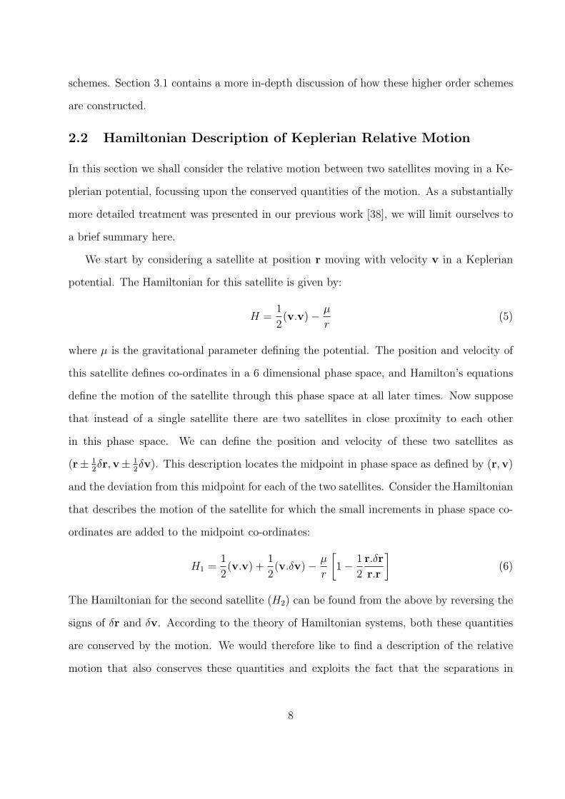
2.2 Hamiltonian Description of Keplerian Relative Motion

In this section we shall consider the relative motion between two satellites moving in a Ke-

plerian potential, focussing upon the conserved quantities of the motion. As a substantially

more detailed treatment was presented in our previous work [38], we will limit ourselves to

a brief summary here.

We start by considering a satellite at position r moving with velocity v in a Keplerian

potential. The Hamiltonian for this satellite is given by:

H =1

2(v.v)− µ

r(5)

where µ is the gravitational parameter defining the potential. The position and velocity of

this satellite defines co-ordinates in a 6 dimensional phase space, and Hamilton’s equations

define the motion of the satellite through this phase space at all later times. Now suppose

that instead of a single satellite there are two satellites in close proximity to each other

in this phase space. We can define the position and velocity of these two satellites as

(r± 12δr,v± 1

2δv). This description locates the midpoint in phase space as defined by (r,v)

and the deviation from this midpoint for each of the two satellites. Consider the Hamiltonian

that describes the motion of the satellite for which the small increments in phase space co-

ordinates are added to the midpoint co-ordinates:

H1 =1

2(v.v) +

1

2(v.δv)− µ

r

[1− 1

2

r.δr

r.r

](6)

The Hamiltonian for the second satellite (H2) can be found from the above by reversing the

signs of δr and δv. According to the theory of Hamiltonian systems, both these quantities

are conserved by the motion. We would therefore like to find a description of the relative

motion that also conserves these quantities and exploits the fact that the separations in

8

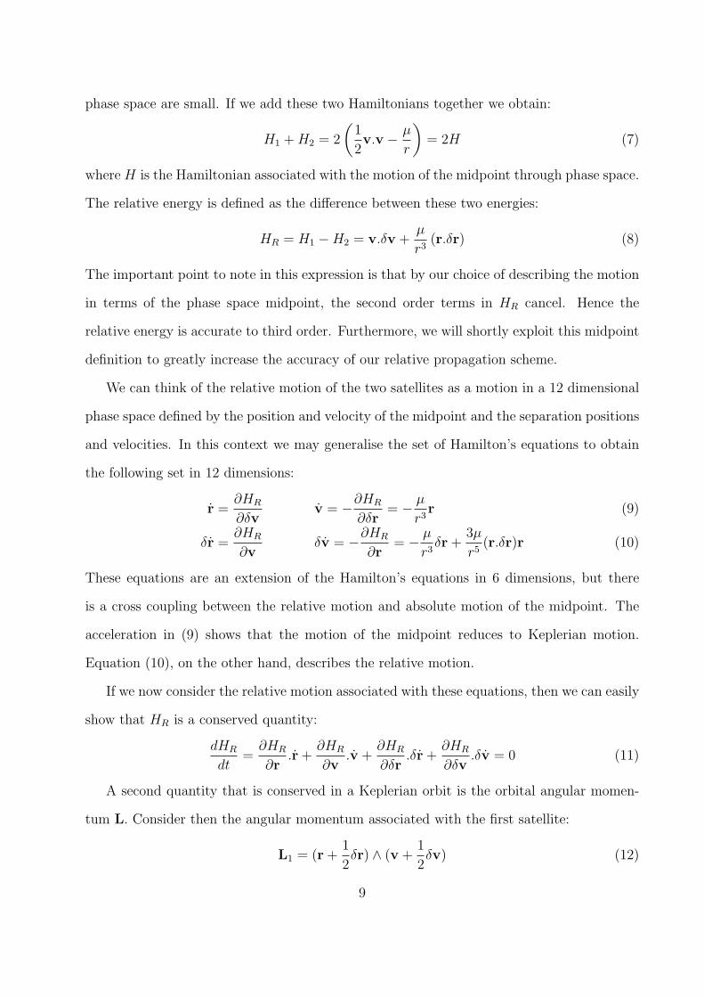
phase space are small. If we add these two Hamiltonians together we obtain:

H1 + H2 = 2

(1

2v.v − µ

r

)= 2H (7)

where H is the Hamiltonian associated with the motion of the midpoint through phase space.

The relative energy is defined as the difference between these two energies:

HR = H1 −H2 = v.δv +µ

r3(r.δr) (8)

The important point to note in this expression is that by our choice of describing the motion

in terms of the phase space midpoint, the second order terms in HR cancel. Hence the

relative energy is accurate to third order. Furthermore, we will shortly exploit this midpoint

definition to greatly increase the accuracy of our relative propagation scheme.

We can think of the relative motion of the two satellites as a motion in a 12 dimensional

phase space defined by the position and velocity of the midpoint and the separation positions

and velocities. In this context we may generalise the set of Hamilton’s equations to obtain

the following set in 12 dimensions:

r =∂HR

∂δvv = −∂HR

∂δr= − µ

r3r (9)

δr =∂HR

∂vδv = −∂HR

∂r= − µ

r3δr +

3µ

r5(r.δr)r (10)

These equations are an extension of the Hamilton’s equations in 6 dimensions, but there

is a cross coupling between the relative motion and absolute motion of the midpoint. The

acceleration in (9) shows that the motion of the midpoint reduces to Keplerian motion.

Equation (10), on the other hand, describes the relative motion.

If we now consider the relative motion associated with these equations, then we can easily

show that HR is a conserved quantity:

dHR

dt=

∂HR

∂r.r +

∂HR

∂v.v +

∂HR

∂δr.δr +

∂HR

∂δv.δv = 0 (11)

A second quantity that is conserved in a Keplerian orbit is the orbital angular momen-

tum L. Consider then the angular momentum associated with the first satellite:

L1 = (r +1

2δr) ∧ (v +

1

2δv) (12)

9

As with the energy, expanding this to first order and differencing for the two satellites we

can write a linearised but third order accurate ‘relative angular momentum’:

LR = L1 − L2 = r ∧ δv − v ∧ δr (13)

Taking the time derivative, it can be easily shown that this relative angular momentum is

also conserved.

2.3 Setting up the Reference Satellite Initial Conditions

In [38], we have shown that, for higher accuracy, we can initialise the reference satellite via

averaging the orbit elements of the two satellites, rather than directly averaging the positions

and velocities. Consequently, the reference satellite motion approximates the motion of the

geometric midpoint to second order; furthermore, HR and LR expressions become accurate

to second order as well.

The expressions for HR and LR (Equations (8) and (13), respectively) point out to the

fact that these quantities approximate the true energy and angular momentum differences,

which are the real quantities that should be conserved. Since the relative position and

velocity of the two satellites are fixed, we need to adjust the position and velocity of the

reference point. The orbital parameters for the reference, however, were fixed in the previous

section. Nevertheless, we have freedom to adjust the true anomaly of the reference point

along that orbit as well as the argument of perigee of the orbit, ω.

The HR and LR terms can thus be adjusted via first order corrections:

H1 −H2 = HR +∂HR

∂θ∆θ +

∂HR

∂ω∆ω (14)

L1 − L2 = LR +∂LR

∂θ∆θ +

∂LR

∂ω∆ω (15)

where ∆θ and ∆ω are small true anomaly and argument of perigee corrections and H1−H2

and L1 − L2 are true energy and angular momentum differences. As all the other terms are

known, we can solve for the ∆θ and ∆ω and calculate the corrections required via these two

10

equations. In the actual implementation, this correction needs to be made only once at the

beginning.

Obviously, for smaller eccentricities, the effect of ω becomes very small and we are unable

to match both HR and LR at the same time. In this case we may need to restrict ourselves

to correcting HR only. If we fix the value of HR to the correct value then we need to solve

a non-linear equation for θ and ω, but in practice a linearised approximation will suffice as

the adjustments in these angles will be small.

2.4 Relative Motion with Perturbations

In the previous two sections we showed how the equations of motion can be written for the

relative motion in a Keplerian potential using the Hamiltonian description. We will now

generalise this method for a geopotential with an arbitrary number of terms in the spherical

harmonics. For this, we introduce the total gravitational potential U(r) such that:

U(r) = −µ

r+ R(r) (16)

The Hamiltonian for a single satellite was given in Equation (1). In a similar fashion, we

can generalise (6) as:

H1 =1

2

(v +

1

2δv

).

(v +

1

2δv

)+ U(r +

1

2δr) (17)

Since our satellites are moving in close proximity to each other, then we may expand the

potential functions in a Taylor series about the midpoint location r. Ignoring terms of order

O(δr3) the Hamiltonian becomes:

H1 =1

2

[v.v + (v.δv) +

1

4(δv.δv)

]+

[U(r) +

1

2

∂U(r)

∂rδr +

1

8

∂2U(r)

∂r2(δr)(δr)T

](18)

The Hamiltonian for the second satellite (H2) can be found from the above by reversing

the signs of δr and δv. As in the Keplerian case, H1 and H2 are conserved by the motion.

It can be easily shown that H1 + H2 = 2H for this generalised case.

11

If we now subtract the expanded H1 and H2 expressions, we obtain the relative Hamil-

tonian:

HR = (v.δv) +∂U(r)

∂rδr (19)

which is simply the generalised form of (8). We can take the Hamilton’s Equations to obtain:

r =∂HR

∂δvv = −∂HR

∂δr= −∂U(r)

∂r(20)

δr =∂HR

∂vδv = −∂HR

∂r= −∂2U(r)

∂r2δr (21)

Conservation of the relative Hamiltonian HR can be shown in exactly the same way as (11).

3 Symplectic Relative Orbit Propagation

3.1 Numerical Integration Scheme

We have described the motion of a pair of satellites in similar orbits by describing the motion

in terms of a nominal position and velocity and the relative motion between the satellites.

By combining these descriptions we can determine the position and velocity of each satellite

in turn. In this section we shall describe how both these motions are propagated numerically.

The procedure is very similar to the symplectic scheme introduced for the absolute orbit (2.1).

We will make extensive use of the Hamiltonian splitting technique, where the Hamiltonian

can be written as the sum of more than one surrogate Hamiltonians [35]. In our case, we

can first split the Hamiltonian into Keplerian part and perturbations.

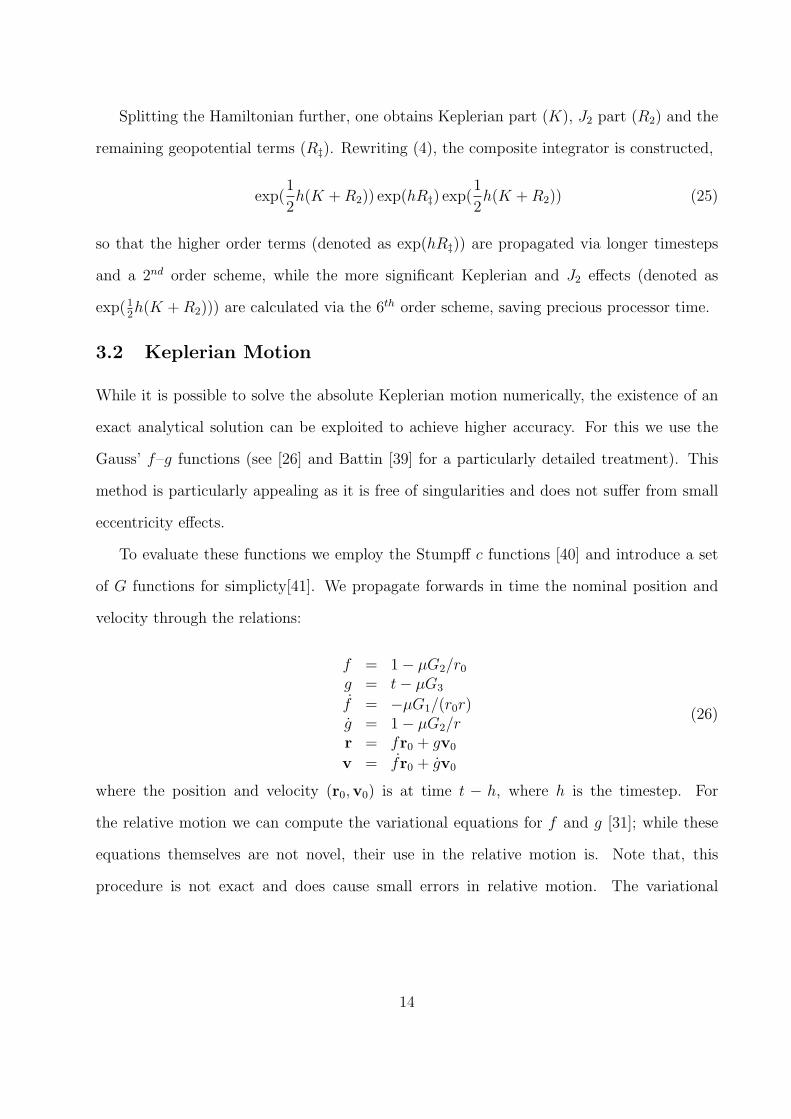
While the Keplerian motion can be modelled via analytical means (see the following

section), the effects of the higher order geopotential terms still need to be propagated nu-

merically. Equation (3) shows the nominal velocity jump due to a non-spherical Earth. For

the relative velocity jump over a full timestep, we can write:

∆δv = −h∂2R

∂r2δr (22)

The numerical integration scheme described in Equation (4) is a second order algorithm,

12

but it is possible to construct higher order schemes in the following form [37]:

exp(xmhK) exp(wmhR) . . . exp(x0hK) exp(w0hR) exp(x0hK) . . . exp(wmhR) exp(xmhK)

(23)

where xm = wm/2, xm−1 = (wm + wm−1)/2, ..., x0 = (w1 + w0)/2.

As long as the perturbations are first order, these methods will have similar orders to

the error of the associated numerical integration formula. This condition is satisfied for the

case of satellites orbiting the Earth, as the Keplerian potential is 103 times larger than the

largest term in the perturbation, which is J2. Therefore, the order of the scheme is O(J2h6).

For the 6th order scheme, Yoshida [34] reports that there are three solutions for wm but

the one with smallest error is:

w1 = −1.17767998417887100695w2 = 0.23557321335935813368w3 = 0.78451361047755726382w0 = 1− 2(w1 + w2 + w3)

(24)

Yoshida [34] obtained these solutions via numerically solving a set of three algebraic equations

simultaneously. We have fully reproduced the coefficients from Leimkuhler and Reich [35]

who presented higher precision results for the same coefficients in comparison to Yoshida [34].

Higher order schemes require greater number of force calculations per integration step.

In fact in the 2nd order scheme requires a single force calculation whereas this increases to

seven force calculations for the 6th order scheme.

The above 6th order integration scheme yields accurate results, however the force due to

the higher order geopotentials has to be computed seven times at each timestep, causing a

significant computational burden. Furthermore, the gains are arguably very small. The J2

term is already an order of magnitude smaller than the two-body force field; the remaining

geopotential terms are at least an order of magnitude smaller than J2, though requiring

much more complicated and lengthy calculations. The solution to this problem comes in the

form of composite schemes, where, for example, high order integration for more significant

terms can be combined with a low order integration for higher order terms.

13

Splitting the Hamiltonian further, one obtains Keplerian part (K), J2 part (R2) and the

remaining geopotential terms (R‡). Rewriting (4), the composite integrator is constructed,

exp(1

2h(K + R2)) exp(hR‡) exp(

1

2h(K + R2)) (25)

so that the higher order terms (denoted as exp(hR‡)) are propagated via longer timesteps

and a 2nd order scheme, while the more significant Keplerian and J2 effects (denoted as

exp(12h(K + R2))) are calculated via the 6th order scheme, saving precious processor time.

3.2 Keplerian Motion

While it is possible to solve the absolute Keplerian motion numerically, the existence of an

exact analytical solution can be exploited to achieve higher accuracy. For this we use the

Gauss’ f–g functions (see [26] and Battin [39] for a particularly detailed treatment). This

method is particularly appealing as it is free of singularities and does not suffer from small

eccentricity effects.

To evaluate these functions we employ the Stumpff c functions [40] and introduce a set

of G functions for simplicty[41]. We propagate forwards in time the nominal position and

velocity through the relations:

f = 1− µG2/r0

g = t− µG3

f = −µG1/(r0r)g = 1− µG2/rr = fr0 + gv0

v = fr0 + gv0

(26)

where the position and velocity (r0,v0) is at time t − h, where h is the timestep. For

the relative motion we can compute the variational equations for f and g [31]; while these

equations themselves are not novel, their use in the relative motion is. Note that, this

procedure is not exact and does cause small errors in relative motion. The variational

14

equations for the Keplerian update can be expressed as:

δf = µG2 δr0/r20 − µδG2/r0

δg = −µδG3

δf = −µδG1/(r0 r) + µG1(δr0/r0 + δr/r)/(r r0)

δg = −µδG2/r + µG2 δr/r2

δr = f δr0 + g δv0 + r0 δf + v0 δg

δv = f δr0 + g δv0 + r0 δf + v0 δg

(27)

This completes the Keplerian update for the nominal and relative positions and velocities.

Note that we will call this the δf − δg method for relative Keplerian motion.

Malhotra [25] has proposed a modification to the f–g functions to include a simple drag

model with a force acting on the alongtrack direction. While we have not implemented

it in our propagator, this model can be easily adapted into relative drag via taking the

variations. Strictly speaking, once the drag is taken into account, a numerical scheme is no

longer symplectic as the system becomes dissipative.

4 Results

4.1 Conservation of Energy

We can show that the relative energy is an oscillation around a stable mean and this oscilla-

tion amplitude goes to zero as the timesteps get smaller. The condition for this is that the

geopotential model is axisymmetric i.e., we take into account zonal harmonics only. Simi-

larly, for such a geopotential model, the z component of the relative angular momentum is

conserved as well.

Firstly, we will show that the relative energy and the z component of the relative angular

momentum are zero mean oscillations. We will use an example where we have one satellite

at 9567.2km semimajor axis and e = 0.3 eccentricity and another in a similar orbit at

23m semimajor axis difference in Keplerian elements. We use an axisymmetric geopotential

containing terms up to J4 only and run the propagation at 100 steps/orbit, for 5 days

15

-2.060e-009

-2.055e-009

-2.050e-009

-2.045e-009

-2.040e-009

-2.035e-009

-2.030e-009

-2.025e-009

-2.020e-009

-2.015e-009

-2.010e-009

-2.005e-009

0 1 2 3 4 5

HR

(no

ndim

)

time (days)

HR

Figure 1: Variation of the HR with J4 level zonal and tesseral harmonics

(46 orbits). Figure 1 shows the variation of HR, which is seen to be oscillating around a

stable mean, with an amplitude of 4.8× 10−11. This shows that HR is indeed conserved.

Secondly, we will show that the z component of the relative angular momentum is con-

served. Figure 2 shows its variation for the same as example as above, compared to its initial

value. This is just a random walk with an error at 10−16 level, which is down to machine

accuracy. Therefore, conservation of the z component of the angular momentum is shown

for the relative motion.

We can use this test setup to illustrate how fast the relative energy oscillation ampli-

tude decreases as integration timesteps are made smaller. We also would like to investigate

whether this decrease rate is any different as compared to running two absolute propaga-

tions and taking the difference of the calculated energies. It should be emphasised that this

oscillation amplitude is an indicator of the positional accuracy as well.

Figure 3 shows the variation of oscillation amplitudes in H, H1−H2 and HR for various

stepsizes. As can be expected, the oscillation in H is about an order of magnitude larger

than that of the relative motion. For all cases, with increasing number of steps per orbit, we

can see the diminishing returns in oscillation amplitude decrease rate. This suggests that,

in practice, very small stepsizes will be of limited use.

16

-2.00e-017

0.00e+000

2.00e-017

4.00e-017

6.00e-017

8.00e-017

1.00e-016

0 1 2 3 4 5

z ax

is r

elat

ive

ang

mom

err

or (

nond

im)

time (days)

delta Lz

Figure 2: Conservation of relative angular momentum - z component

1.00e-013

1.00e-012

1.00e-011

1.00e-010

1.00e-009

1.00e-008

1.00e-007

0 100 200 300 400 500 600 700 800 900 1000

ener

gy o

scill

atio

n am

plitu

de (

nond

im)

number of steps/orbit

HHR

H1-H2

Figure 3: Energy oscillation amplitude (log scale) in H, H1 − H2 and HR for various inte-gration stepsizes

17

a(km) e I(deg) Ω(deg) ω(deg) θ(deg) H LSat1 7653.780 0.0050 60.00 40.0 20.0 240.0 -0.416665 1.095432Sat2 7653.700 0.0055 60.01 40.0 19.0 241.0 -0.416667 1.095426Diff -0.080 0.0005 0.010 0.0 -1.0 1.0 −2.17× 10−6 −5.73× 10−6

Table 1: Integration test case initial conditions in Keplerian elements

Comparing the difference in energies H1−H2 and the relative Hamiltonian HR, we see that

their oscillation amplitudes decrease at a very similar rate, which suggests that very similar

accuracies can be obtained by running the relative orbit propagator or differencing the results

of two absolute propagations. However, for a geopotential model with 36 terms in the zonal

and tesseral harmonics, the relative orbit propagation is about 40% faster in computational

time than running two absolute orbit propagations. This shows that the relative orbit scheme

yields much better efficiency and is ideal for applications with limited computational power.

However, it must be emphasised that on a computer with AMD2400 CPU and 512MB

memory the runtime is only a few seconds.

4.2 Number of Geopotentials

In this section we will compare the accuracies of geopotential models of different complexity

with a high-precision geopotential model.

We will use the initial conditions given in Table 1 for a 5-day propagation at 120 steps/orbit.

The truth model is a 1000 steps/orbit composite symplectic scheme with a 36×36 geopoten-

tial field model; as before, we calculate the absolute orbit for each satellite with this scheme

and take the difference to obtain the relative orbit.

Figure 4 summarises the relative positioning errors after a five day propagation with ax-

isymmetric and non-axisymmetric geopotential models containing various number of geopo-

tentials. Note that, ‘zero geopotentials’ in the figure correspond to the Keplerian case.

While a higher number of geopotentials increase the accuracy as expected, excluding the

tesseral terms seems to cause a large offset. The total energy difference can be written as a

summation of smaller Hamiltonians due to other geopotential terms i.e., δH = δHK + δH2 +

18

1.00e-004

1.00e-003

1.00e-002

1.00e-001

1.00e+000

1.00e+001

1.00e+002

0 5 10 15 20 25 30 35 40

rel p

os e

rror

(km

)

number of geopotentials

HRLRHRLR axi

df-dgdf-dg axi

Figure 4: Relative positioning error (log scale) with various geopotentials - 5 days (65 orbits)

δH3 + . . . + δHtess, where δHK is the difference in Keplerian potential, δH2 is the difference

in J2 potential, δH3 due to J3 and δHtess due to all tesseral terms. Given the coordinates

of two satellites, different models will obviously yield different δH values. The energy of a

satellite determines the mean motion and the energy difference thus determines the relative

mean motion or relative drift rate. Evidently, a simple model that includes 4 terms in the

geopotential will have a significantly different drift rate with respect to a 36 term model due

to these truncated geopotential terms, hence a large relative positioning error results.

However, the most striking feature of Figure 4 is that δf–δg and HRLR methods yield

virtually the same errors. In fact, the difference between the two methods is less than

10−5 metres for all cases.

From these tests we conclude that, for a given set of formation initial conditions, it is

possible to obtain metre level accuracy after 5 days with about 20 geopotentials included

in the model. More importantly, we showed that the two analytical methods for Keplerian

relative orbit propagation are practically equivalent.

19

a(km) e I(deg) Ω(deg) ω(deg) θ(deg) H LSat1 15945.80 0.3500 60.00 40.03 20.00 70.00 -0.199994 1.481152Sat2 15945.65 0.3501 60.03 40.03 19.95 70.05 -0.199996 1.481086Diff -0.15 0.0001 0.030 0.030 -0.050 0.050 −1.88× 10−6 −6.60× 10−5

Table 2: Test case formation initial conditions in Keplerian elements

4.3 Relative Positioning Accuracy

We will demonstrate the relative positioning accuracy for a range of eccentricities. We also

would like to show that the two relative propagation methods (δf − δg method and HRLR

method presented in [38]) will yield practically the same results as they are both first order

approximations to the relative motion.

The first set of tests will use the initial conditions given in Table 2 to run 5 day (21.5 orbit)

simulations. We will start with a Keplerian model to compare the two analytical relative

orbit models. The initial separations range from 5.8km for e = 0.55 to 9km for near-circular

cases. Peak separations range from 54km for e = 0.55 to 34km for near-circular cases.

Figure 5 illustrates the relative positioning error for this case through a range of eccen-

tricities. As can be seen, the two methods yield virtually the same results, proving further

that they are practically equivalent. The difference between the two remains around 10−7

metres, regardless of the eccentricity.

The second set of tests is to repeat the above but with a 36× 36 geopotential model and

two stepsizes: 100 steps/orbit and 300 steps/orbit. The truth model is 1000 steps/orbit.

Figure 6 shows the results for this test case, where the HRLR or df − dg denotes the method

and 100 or 300 denotes the number of steps/orbit in the figure caption. As expected, the

two methods yield practically identical results with differences around 10−7 metres or less.

While the relative positioning accuracy is very high for both 100 and 300 steps/orbit cases,

the former start to become unstable at around e = 0.5. For the latter, while the errors

increase with eccentricity, they stay well below metre level.

20

1.00e-006

1.00e-005

1.00e-004

1.00e-003

0.05 0.1 0.15 0.2 0.25 0.3 0.35 0.4 0.45 0.5 0.55

rel p

os e

rror

(km

)

eccentricity

df-dgHRLR

Figure 5: Relative positioning error (log scale) with eccentricity for Keplerian potential - 5days (21.5 orbits)

1.00e-006

1.00e-005

1.00e-004

1.00e-003

1.00e-002

1.00e-001

0.05 0.1 0.15 0.2 0.25 0.3 0.35 0.4 0.45 0.5 0.55

rel p

os e

rror

(km

)

eccentricity

df-dg 100HRLR 100df-dg 300HRLR 300

Figure 6: Relative positioning error (log scale) with eccentricity for 36 × 36 potential - 5days (21.5 orbits)

21

0 10 20 30 40 50 0.0

0.1

0.2

0.3

0.4

0.5

0.6

0.7

0.8

0.9

1.0

rel p

os e

rror

(km

)

perc

enta

ge r

el p

os e

rror

time (days)

err% err

Figure 7: Relative positioning error (log scale) in 50 days (650 orbits)

4.4 Long-term Stability

In the previous sections we showed that the algorithm works remarkably well for durations

of several days. However, we would like to demonstrate how it would perform when the

separations are well beyond the close proximity assumption; it is important to see how

quickly the algorithm breaks down.

To this end, we used the initial conditions given in Table 1 but with a 600m semimajor

axis difference rather than 80m. We run a 50 day (650 orbit) propagation with a 36 × 36

geopotential model at a stepsize of 120 steps/orbit. The truth model is at 1000 steps/orbit,

employing the same geopotential model. The separation starts from 1.5km but exceeds

3640km by the end of the simulation run.

Figure 7 shows the relative positioning error both in kilometres and as percentage of

the separation. While the relative positioning error reaches 35km by the end of 50 days,

it corresponds to about 1% of the separation. From this experiment we conclude that the

propagator works extremely well and its accuracy degrades gracefully long after the linearity

assumption has broken down.

22

5 Conclusions

A novel method for propagating a relative orbit with high order geopotentials up to 36× 36

terms has been presented, building upon the heritage of existing symplectic absolute orbit

propagators. The relative propagation is symplectic for the non-Keplerian higher order

geopotentials, whereas the Keplerian part is handled analytically by a novel implementation

of the Gauss’ functions. Also a high performance composite numerical integration scheme

has been set up for better utilisation of the processing power. For a given integration stepsize,

this is about 40% faster than differencing two absolute orbit propagations, for the same level

of accuracy.

The results demonstrate that the propagator can yield metre level or better relative

positioning accuracy after five days even with 36 zonal and tesseral harmonics included in

the geopotential model, without any limitations on eccentricity. It is therefore a significant

step towards relative navigation filters with better dynamic models, requiring much less

sensor inputs.

Acknowledgements

Egemen Imre has been supported by the Turkish Research and Development Agency

TUBITAK-UZAY and Surrey Space Centre throughout this work.

References

[1] Clohessy, W. and Wiltshire, R., “Terminal Guidance System for Satellite Rendezvous,”

Journal of the Aerospace Sciences , Vol. 27, No. 9, 1960, pp. 653–658, 674.

[2] Hill, G. W., “Researches in the Lunar Theory,” American Journal of Mathematics ,

Vol. 1, No. 3, 1878, pp. 5–26, 129–147, 245–260.

[3] Gim, D.-W. and Alfriend, K. T., “The State Transition Matrix for Relative Motion of

Formation Flying Satellites,” AAS Space Flight Mechanics Meeting , San Antonio,

Texas, USA, 2002, AAS 02-186.

23

[4] Gim, D.-W. and Alfriend, K. T., “The State Transition Matrix of Relative Motion for

the Perturbed Non-Circular Reference Orbit,” Advances in the Astronautical Sciences,

Guidance and Control , Vol. 108, American Astronautical Society, 2001, pp. 913–934,

AAS 01-222.

[5] Ross, M., “Linearized Dynamic Equations for Spacecraft Subject to J2 Perturbations,”

Journal of Guidance, Control and Dynamics , Vol. 26, No. 4, 2003, pp. 657–659, Engr’g

note.

[6] Schaub, H. and Alfriend, K. T., “J2 Invariant Relative Orbits for Spacecraft

Formations,” Celestial Mechanics and Dynamical Astronomy , Vol. 79, Feb. 2001,

pp. 77–95.

[7] Schweighart, S. and Sedwick, R., “Perturbative Analysis of Geopotential Disturbances

for Satellite Formation Flying,” Proceedings of the IEEE Aerospace Conference, Vol. 2,

Big Sky, Montana, US, 2001, pp. 1001–1019.

[8] Schweighart, S. and Sedwick, R., “High-Fidelity Linearized J2 Model for Satellite

Formation Flight,” Journal of Guidance, Control and Dynamics , Vol. 25, No. 6, 2002,

pp. 1073–1080.

[9] Broucke, R., “Solution of the Elliptic Rendezvous Problem with the Time as

Independent Variable,” Journal of Guidance, Control and Dynamics , Vol. 26, No. 4,

2003, pp. 615–621.

[10] Inalhan, G., Tillerson, M., and How, J., “Relative Dynamics and Control of Spacecraft

Formations in Eccentric Orbits,” Journal of Guidance, Control and Dynamics ,

Vol. 25, No. 1, 2002, pp. 48–59.

[11] Lawden, D., “Fundamentals of Space Navigation,” Journal of Britsh Interplanetary

Society , Vol. 13, May 1954, pp. 87–101.

24

[12] Melton, R., “Time-Explicit Representation of Relative Motion Between Elliptical

Orbits,” Journal of Guidance, Control and Dynamics , Vol. 23, No. 4, 2000,

pp. 604–610.

[13] Tschauner, J. and Hempel, P., “Optimale Beschleunigeungsprogramme fur das

Rendezvous-Manover,” Acta Astronautica, Vol. 10, No. 5–6, 1964, pp. 296–307.

[14] Carter, T. and Humi, M., “Fuel-Optimal Rendezvous Near a Point in General

Keplerian Orbit,” J. Guidance, Vol. 10, No. 6, 1987, pp. 567–573.

[15] Kormos, T., Dynamics and Control of Satellite Constellations and Formations in Low

Earth Orbit , Ph.D. thesis, University of Surrey, Guildford, UK, 2004.

[16] O’Donnell, K., Satellite Orbits in Resonance with Tesseral Harmonics: Absolute and

Relative Orbit Analysis , Ph.D. thesis, University of Surrey, Guildford, UK, 2005.

[17] Kormos, T. and Palmer, P., “Modelling and Control of Relative Orbits for Spacecraft

Flying in Formation in LEO,” Third International Workshop on Satellite

Constellations and Formation Flying , Pisa, Italy, 2003, pp. 279–286.

[18] Wiesel, W., “Relative Satellite Motion About an Oblate Planet,” Journal of Guidance,

Control and Dynamics , Vol. 25, No. 4, 2002, pp. 776–785.

[19] Karlgaard, C. and Lutze, F., “Second-Order Relative Motion Equations,” Journal of

Guidance, Control and Dynamics , Vol. 26, No. 1, 2003, pp. 41–49.

[20] Melton, R., “Comparison of Relative-Motion Models for Elliptical Orbits,” Proc. Third

International Workshop on Satellite Constellations and Formation Flying , Pisa, Italy,

2003.

[21] Alfriend, K. and Yan, H., “Evaluation and Comparison of Relative Motion Theories,”

Journal of Guidance, Control and Dynamics , Vol. 28, No. 2, 2005, pp. 254–261.

25

[22] Bate, R., Mueller, D., and White, J., Fundamentals of Astrodynamics , Dover

Publications, Inc, New York, USA, 1971.

[23] Busse, F. D., Simpson, J., and How, J. P., “Demonstration of Adaptive Extended

Kalman Filtering for LEO Formation Estimation Using CDGPS,” Navigation Journal

of the Institute of Navigation, Vol. 50, No. 2, 2003, pp. 79–94.

[24] Inalhan, G., Busse, F., and How, J., “Precise Formation Flying Control of Multiple

Spacecraft using Carrier-Phase Differential GPS,” Proceedings of the AAS/AIAA

Space Flight Mechanics Meeting , Clearwater, Florida, USA, 2000.

[25] Malhotra, R., “A Mapping Method for the Gravitational Few-Body Problem with

Dissipation,” Celestial Mechanics and Dynamical Astronomy , Vol. 60, No. 3, 1994,

pp. 373–385.

[26] Vallado, D. A., Fundamentals of Astrodynamics and Applications , Microcosm, Inc,

2nd ed., 2001.

[27] Montenbruck, O. and Gill, E., Satellite Orbits - Models, Methods and Applications ,

Springer, Heidelberg, Germany, 2001.

[28] Palmer, P., Aarseth, S., Mikkola, S., and Hashida, Y., “High Precision Integration

Methods for Orbit Modelling,” J. of Astronautical Sciences , Vol. 46, No. 4, 1999,

pp. 329–342.

[29] Kinoshita, H. and Yoshida, H. a. N. H., “Symplectic Integrators and their Application

in Dynamical Astronomy,” Celest. Mech. Dyn.Ast., Vol. 50, 1991, pp. 59–71.

[30] Mikkola, S., “Efficient Symplectic Integration of Satellite Orbits,” Celestial Mechanics

and Dynamical Astronomy , Vol. 74, No. 4, 1999, pp. 275–285.

26

[31] Mikkola, S., Palmer, P., and Hashida, Y., “A Symplectic Orbital Estimator for Direct

Tracking on Satellites,” Journal of Astronautical Sciences , Vol. 48, No. 1, 2001,

pp. 109–125.

[32] Palacios, M., “Symplectic versus Other Propagators in the Ideal Formulation of the

Earth Satellite Problem,” Proc. Intern. Symposium Space Dynamics , Biarritz, France,

2000, MS00–36.

[33] Wisdom, J. and Holman, M., “Symplectic Maps for the N-Body Problem,” Astron. J ,

Vol. 102, 1991, pp. 2022–2029.

[34] Yoshida, H., “Construction of Higher Order Symplectic Integrators,” Physics Letters

A, Vol. 150, Nov. 1990, pp. 262–268.

[35] Leimkuhler, B. and Reich, S., Simulating Hamiltonian Dynamics , Cambridge

University Press, Cambridge, UK, 2004.

[36] Goldstein, H., Poole, C., and Safko, J., Classical Mechanics , Addison-Wesley, 3rd ed.,

2002.

[37] Mikkola, S. and Palmer, P., “Simple derivation of Symplectic Integrators with First

Order Correctors,” Celestial Mechanics and Dynamical Astronomy , Vol. 77, Aug.

2000, pp. 305–317.

[38] Palmer, P. and Imre, E., “Relative Motion between Satellites on Neighbouring

Keplerian Orbits,” Journal of Guidance, Control and Dynamics , Accepted for

publication.

[39] Battin, R., An Introduction to the Mathematics and Methods of Astrodynamics , AIAA

Education Series, AIAA, Virgina, USA, rev. ed. ed., 1999.

[40] Stumpff, K., Himmelsmechanik , Band I, VEB Deutscher Verlag der Wissenschaften,

Berlin, Germany, 1962.

27

[41] Stiefel, E. L. and Scheifele, G., Linear and Regular Celestial Mechanics , Springer,

Berlin, Germany, 1971.

28