NATURE BIOTECHNOLOGY VOLUME 24 NUMBER 8 AUGUST 2006 963
High-resolution computational models of genome binding eventsYuan Qi1,6, Alex Rolfe1,6, Kenzie D MacIsaac1,6, Georg K Gerber1,2, Dmitry Pokholok3, Julia Zeitlinger3,Timothy Danford1, Robin D Dowell1, Ernest Fraenkel1,4, Tommi S Jaakkola1, Richard A Young3,5 &David K Gifford1,3
Direct physical information that describes where transcription factors, nucleosomes, modified histones, RNA polymerase II and other key proteins interact with the genome provides an invaluable mechanistic foundation for understanding complex programs of gene regulation. We present a method, joint binding deconvolution (JBD), which uses additional easily obtainable experimental data about chromatin immunoprecipitation (ChIP) to improve the spatial resolution of the transcription factor binding locations inferred from ChIP followed by DNA microarray hybridization (ChIP-Chip) data. Based on this probabilistic model of binding data, we further pursue improved spatial resolution by using sequence information. We produce positional priors that link ChIP-Chip data to sequence data by guiding motif discovery to inferred protein-DNA binding sites. We present results on the yeast transcription factors Gcn4 and Mig2 to demonstrate JBD’s spatial resolution capabilities and show that positional priors allow computational discovery of the Mig2 motif when a standard approach fails.
ChIP-Chip has emerged as a powerful tool for studying in vivo genome-wide protein-DNA interactions including transcription factor binding1–13, DNA replication and recombination14,15 and nucleosome occupancy and histone modification state16–22. Such information has been used to discover transcription factor–DNA binding motifs, to predict gene expression and to construct large-scale regulatory network models10,20,21,23–27. Supplementary Figure 1 online shows the ChIP-Chip experimental procedure.
Because raw ChIP-Chip data are complex and noisy28, computa-tional methods are necessary for extracting meaningful informa-tion. Researchers analyzing these data are typically interested in
discovering distinct binding events, which we define as localized inter-actions between proteins and DNA. We further define spatial resolution to be the distance between an inferred binding event location and its true location. An ideal computational method would accurately local-ize inferred binding events (high spatial resolution), would include no false binding events (high specificity) and would not miss true binding events (high sensitivity).
We propose JBD as a computational approach that reconstructs binding events from ChIP-Chip data at a higher spatial resolution than the underlying microarray probe spacing. Because a binding event influences multiple proximal microarray probes, we can decon-volve the predicted probe intensity peak shape from the observed peak shape to infer the true binding event location. Our method jointly considers all possible configurations of binding events, allowing pairs of nearby events to be distinguished more reliably than by other meth-ods. Additional detailed information about binding events is obtained by incorporating sequence data. We do this by linking JBD to DNA motif discovery. JBD’s high-resolution output is used to compute a positional prior for a DNA sequence motif ’s existence at each base pair, which guides the motif-discovery algorithm to small regions of DNA sequence. By focusing on regions that are tens of bases in size rather than hundreds or thousands, the motif-discovery algorithm becomes more resistant to ambiguous and noisy inputs.
Previous ChIP-Chip analysis methods have not attempted to improve the underlying microarray’s spatial resolution and have not used an experimentally determined peak shape. The simplest analysis method for ChIP-Chip data infers binding events at those probes that have intensities above a specified threshold. Better methods have gen-erally used statistical techniques to identify bound promoter regions or windows of enriched probes11,21,28–30. One method, MPeak, fits a hypothesized shape to ChIP-Chip probe intensities, but does not consider multiple binding events jointly or attempt to increase the underlying microarray’s spatial resolution31. See the Supplementary Discussion online for more on previous work.
We demonstrate our method on the yeast transcription factors Gcn4 and Mig2. Using evolutionarily conserved instances of a previ-ously published Gcn4 sequence motif to define plausible target genes, we show that JBD makes more accurate binding predictions with higher sensitivity and specificity than do three competing methods. We show that using JBD’s output as a positional prior allows motif discovery to ignore erroneous input sequences. We use JBD-derived
1MIT Computer Science and Artificial Intelligence Laboratory, 32 Vassar Street, Cambridge, Massachusetts 02139, USA. 2Harvard-MIT Division of Health Sciences and Technology, 45 Carleton Street Room E25-519, Cambridge, Massachusetts 02139, USA. 3Whitehead Institute for Biomedical Research, Nine Cambridge Center, Cambridge, Massachusetts 02142, USA. 4MIT Biological Engineering Division, 77 Massachusetts Ave., Cambridge, Massachusetts 02139, USA. 5MIT Department of Biology, 31 Ames Street Room 68-132, Cambridge, Massachusetts 02139, USA. 6These authors contributed equally to the work. Correspondence should be addressed to D.K.G. ([email protected]).
Published online 9 August 2006; doi:10.1038/nbt1233
964 VOLUME 24 NUMBER 8 AUGUST 2006 NATURE BIOTECHNOLOGY
positional priors from Mig2 binding data to find a correct binding site motif, which other computational methods have been unable to do. To examine JBD’s performance without any uncertainty about the true binding event locations, we generated several synthetic data sets based on the Gcn4 data. We use these data sets to compare JBD to several other methods and to examine JBD’s performance on different ChIP-Chip microarray designs.
RESULTSWe formulate the problem of detecting binding events as a prob-abilistic graphical model that captures the combined effect of multiple binding events on each microarray probe. Our model is generative, because we specify how an underlying physical process
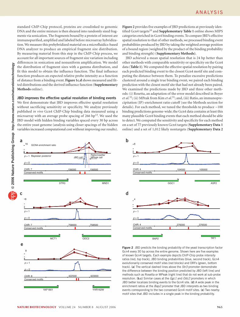
probabilistically generates the experimental data. In particular, we model DNA fragmentation in the ChIP-Chip protocol (Fig. 1a). The fragmentation process produces pieces of DNA of varying sizes at a given binding event locus and the genomic interval covered by a given fragment determines what probes it influences. JBD uses an experimentally measured distribution of fragment sizes to predict the probe intensity peak shape that a binding event will produce, and then fits this shape to ChIP-Chip data to infer binding event locations. Figure 1b provides a summary of the model.
Modeling the effect of binding events on proximal probe intensityWe derive an influence function to model the contribution of DNA fragments to intensities of probes proximal to a binding event. In the
Shear
Hybridize
Microarrayreadout
Further samplepreparation
Observedratio
Strength
Indicator
Probability
Inferredbinding
variables
yi
sj
bj
πj
1
0.8
0.6
0.4
0.2
0
1
0.8
0.6
0.4
0.2
00 500 1,000
Fragment length–500 0 500
Genomic distance
Rel
ativ
e co
ncen
trat
ion
Rel
ativ
e pr
obe
inte
nsity
a b
c d
Figure 1 JBD probabilistically models key aspects of ChIP-Chip experiments. (a) Key aspects of the ChIP-Chip protocol involve (i) shearing of DNA crosslinked to a protein, (ii) immunoprecipitation of bound fragments and (iii) hybridization of the fragments to a microarray and the resulting data readout. (b) JBD is a generative probabilistic graphical model, depicted using standard Bayesian Network notation. The unobserved (hidden) binding variables at the bottom affect the observed data (probe intensity measurements yi, the top row of circles) through an influence function. For a given genomic location j, we model the prior probability of protein-DNA binding (πj), the binding event (bj) and a continuous binding strength (sj). (c) The distribution of DNA fragment sizes produced in the ChIP protocol were experimentally measured and statistically modeled. The measured distribution from binding experiments using the yeast transcriptional activator Gcn4 is shown (blue) with the fitted statistical model (red). The mean fragment size is 327 bp. (d) An influence function is derived from the measured fragment size distribution, specifying the expected relative probe intensity as a function of distance from a binding event.
NATURE BIOTECHNOLOGY VOLUME 24 NUMBER 8 AUGUST 2006 965
standard ChIP-Chip protocol, proteins are crosslinked to genomic DNA and the entire mixture is then sheared into randomly sized frag-ments via sonication. The fragments bound by a protein of interest are immunopurified, amplified and labeled before microarray hybridiza-tion. We measure this prehybridized material on a microfluidics-based DNA analyzer to produce an empirical fragment size distribution. By measuring material from this step in the ChIP-Chip process, we account for all important sources of fragment size variation including differences in sonication and nonuniform amplification. We model the distribution of fragment sizes with a gamma distribution, and fit this model to obtain the influence function. The final influence function produces an expected relative probe intensity as a function of distance from a binding event. Figure 1c,d shows measured and fit-ted distributions and the derived influence function (Supplementary Methods online).
JBD improves the effective spatial resolution of binding eventsWe first demonstrate that JBD improves effective spatial resolution without sacrificing sensitivity or specificity. We analyze previously published in vivo Gcn4 ChIP-Chip binding data measured using a microarray with an average probe spacing of 266 bp13. We used the JBD model with hidden binding variables spaced every 30 bp across the entire yeast genome (analysis using closer spacings of the hidden variables increased computational cost without improving our results).
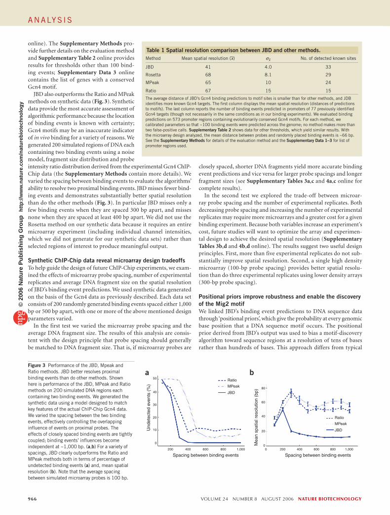
Figure 2 provides five examples of JBD predictions at previously iden-tified Gcn4 targets10 and Supplementary Table 1 online shows MIPS categories enriched in Gcn4 binding events. To compare JBD’s effective spatial resolution to that of other methods, we processed binding event probabilities produced by JBD by taking the weighted average position of a bound region (weighted by the product of the binding probability and binding strength) (Supplementary Methods).
JBD achieved a mean spatial resolution that is 24 bp better than other methods with comparable sensitivity or specificity on the Gcn4 data (Table 1). We computed the effective spatial resolution by pairing each predicted binding event to the closest Gcn4 motif site and com-puting the distance between them. To penalize excessive predictions clustered around a single true binding event, we paired each binding prediction with the closest motif site that had not already been paired. We examined the predictions made by JBD and three other meth-ods: (i) Rosetta, an adaptation of the error model described in Boyer et al.32; (ii) MPeak from Kim et al.31; and, (iii) Ratio, an immunopre-cipitation (IP)-enrichment ratio cutoff (see the Methods section for details). For each method, we tuned the thresholds to produce ~100 binding predictions genome-wide; the Gcn4 data contains at least this many plausible Gcn4 binding events that each method should be able to detect. We computed the sensitivity and specificity for each method on a set of 77 previously known Gcn4 targets (Supplementary Data 1 online) and a set of 1,012 likely nontargets (Supplementary Data 2
16 GCN4 enrichment ratio
Bayesian posterior
Conserved motifs
p = 1
p = 0
CHR: 7
JBD callRatio/rosetta/MPeak call
156000 156500
STR3 MND1
8
Conserved motifs
p = 1
p = 0
CHR: 4
GGC1 ASF2
104500 105000
8
Conserved motifs
p = 1
p = 0
CHR: 7
MCT1 ODC2
758000 758500
4
Conserved motifs
p = 1
p = 0
CHR: 4 376000 376500
BAP2 TAT1
8
Conserved motifs
p = 1
p = 0
CHR: 8
YAP1801 YHR162W
422500 423000
a b
c d
eFigure 2 JBD predicts the binding probability of the yeast transcription factor Gcn4 every 30 bp across the entire genome. Shown here are five examples of known Gcn4 targets. Each example depicts ChIP-Chip probe intensity ratios (red, top track), JBD binding probabilities (blue, second track), Gcn4 evolutionarily conserved motif sites (red blocks) and ORFs (green, bottom track). (a) The vertical dashed lines above the Str3 promoter demonstrate the difference between the binding position predicted by JBD (left line) and methods such as Rosetta or MPeak (right line) that do not work at sub-probe resolution. (b,c) Similar cases at the Ggc1 and Odc2 promoters in which JBD better localizes binding events to the Gcn4 site. (d) A wide peak in the enrichment ratios at the Bap2 promoter that JBD interprets as two binding events corresponding to the two conserved Gcn4 motif sites. (e) Two nearby motif sites that JBD includes in a single peak in the binding probability.
966 VOLUME 24 NUMBER 8 AUGUST 2006 NATURE BIOTECHNOLOGY
online). The Supplementary Methods pro-vide further details on the evaluation method and Supplementary Table 2 online provides results for thresholds other than 100 bind-ing events; Supplementary Data 3 online contains the list of genes with a conserved Gcn4 motif.
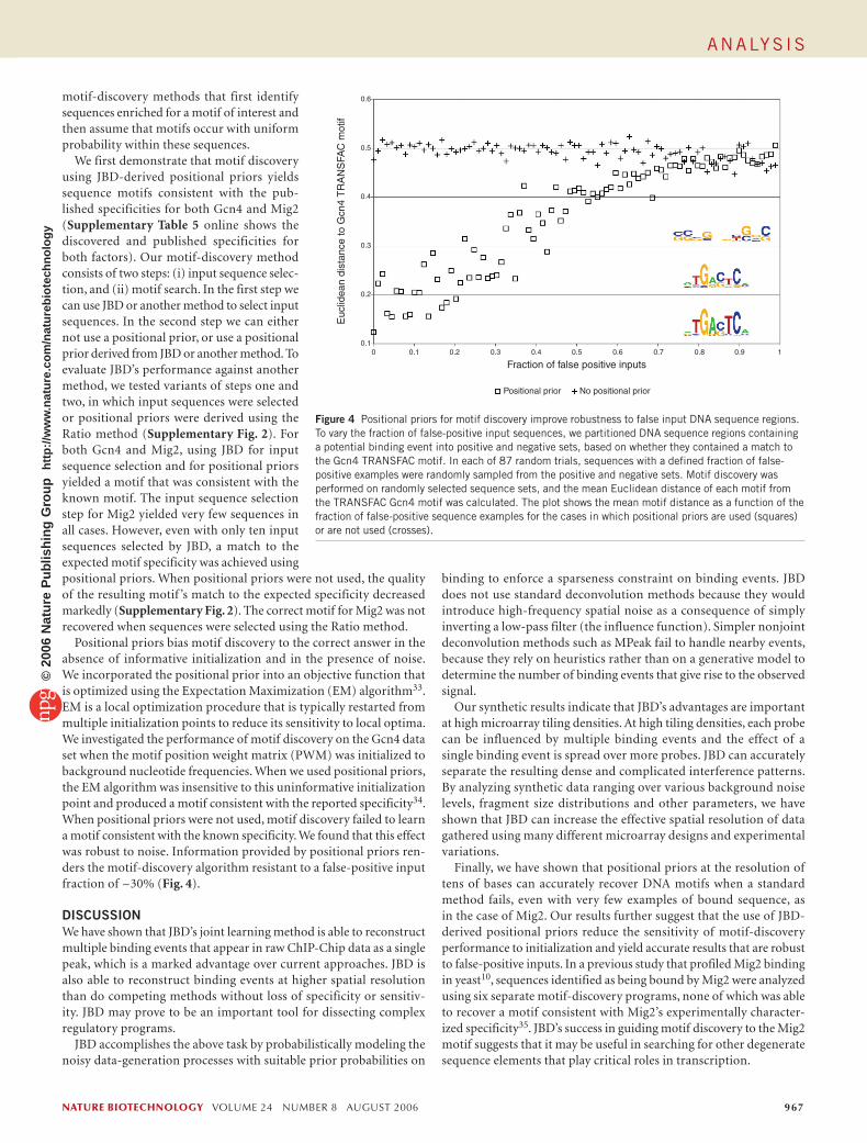
JBD also outperforms the Ratio and MPeak methods on synthetic data (Fig. 3). Synthetic data provide the most accurate assessment of algorithmic performance because the location of binding events is known with certainty; Gcn4 motifs may be an inaccurate indicator of in vivo binding for a variety of reasons. We generated 200 simulated regions of DNA each containing two binding events using a noise model, fragment size distribution and probe intensity ratio distribution derived from the experimental Gcn4 ChIP-Chip data (the Supplementary Methods contain more details). We varied the spacing between binding events to evaluate the algorithms’ ability to resolve two proximal binding events. JBD misses fewer bind-ing events and demonstrates substantially better spatial resolution than do the other methods (Fig. 3). In particular JBD misses only a few binding events when they are spaced 300 bp apart, and misses none when they are spaced at least 400 bp apart. We did not use the Rosetta method on our synthetic data because it requires an entire microarray experiment (including individual channel intensities, which we did not generate for our synthetic data sets) rather than selected regions of interest to produce meaningful output.
Synthetic ChIP-Chip data reveal microarray design tradeoffsTo help guide the design of future ChIP-Chip experiments, we exam-ined the effects of microarray probe spacing, number of experimental replicates and average DNA fragment size on the spatial resolution of JBD’s binding event predictions. We used synthetic data generated on the basis of the Gcn4 data as previously described. Each data set consists of 200 randomly generated binding events spaced either 1,000 bp or 500 bp apart, with one or more of the above mentioned design parameters varied.
In the first test we varied the microarray probe spacing and the average DNA fragment size. The results of this analysis are consis-tent with the design principle that probe spacing should generally be matched to DNA fragment size. That is, if microarray probes are
closely spaced, shorter DNA fragments yield more accurate binding event predictions and vice versa for larger probe spacings and longer fragment sizes (see Supplementary Tables 3a,c and 4a,c online for complete results).
In the second test we explored the trade-off between microar-ray probe spacing and the number of experimental replicates. Both decreasing probe spacing and increasing the number of experimental replicates may require more microarrays and a greater cost for a given binding experiment. Because both variables increase an experiment’s cost, future studies will want to optimize the array and experimen-tal design to achieve the desired spatial resolution (Supplementary Tables 3b,d and 4b,d online). The results suggest two useful design principles. First, more than five experimental replicates do not sub-stantially improve spatial resolution. Second, a single high density microarray (100-bp probe spacing) provides better spatial resolu-tion than do three experimental replicates using lower density arrays (300-bp probe spacing).
Positional priors improve robustness and enable the discovery of the Mig2 motifWe linked JBD’s binding event predictions to DNA sequence data through ‘positional priors’, which give the probability at every genomic base position that a DNA sequence motif occurs. The positional prior derived from JBD’s output was used to bias a motif-discovery algorithm toward sequence regions at a resolution of tens of bases rather than hundreds of bases. This approach differs from typical
Table 1 Spatial resolution comparison between JBD and other methods. Method Mean spatial resolution (x −) σ x − No. of detected known sites
JBD 41 4.0 33
Rosetta 68 8.1 29
MPeak 65 10 24
Ratio 67 15 15
The average distance of JBD’s Gcn4 binding predictions to motif sites is smaller than for other methods, and JDB identifies more known Gcn4 targets. The first column displays the mean spatial resolution (distances of predictions to motifs). The last column reports the number of binding events predicted in promoters of 77 previously identified Gcn4 targets (though not necessarily in the same conditions as in our binding experiments). We evaluated binding predictions on 573 promoter regions containing evolutionarily conserved Gcn4 motifs. For each method, we calibrated parameters so that ~100 binding events were predicted across the genome; no method makes more than two false-positive calls. Supplementary Table 2 shows data for other thresholds, which yield similar results. With the microarray design analyzed, the mean distance between probes and randomly placed binding events is ~66 bp. See the Supplementary Methods for details of the evaluation method and the Supplementary Data 1–3 for list of promoter regions used.
Und
etec
ted
even
ts (
%)
40
50
30
20
10
0
200 400 600 800 1,000
Spacing between binding events
Ratio
MPeak
JBD80
60
40
20
0Mea
n sp
atia
l res
olut
ion
(bp)
2000
Ratio
MPeak
JBD
400 600 800 1,000
Spacing between binding events
a bFigure 3 Performance of the JBD, Mpeak and Ratio methods. JBD better resolves proximal binding events than do other methods. Shown here is performance of the JBD, MPeak and Ratio methods on 200 simulated DNA regions each containing two binding events. We generated the synthetic data using a model designed to match key features of the actual ChIP-Chip Gcn4 data. We varied the spacing between the two binding events, effectively controlling the overlapping influence of events on proximal probes. The effects of closely spaced binding events are tightly coupled; binding events’ influences become independent at ~1,000 bp. (a,b) For a variety of spacings, JBD clearly outperforms the Ratio and MPeak methods both in terms of percentage of undetected binding events (a) and, mean spatial resolution (b). Note that the average spacing between simulated microarray probes is 100 bp.
NATURE BIOTECHNOLOGY VOLUME 24 NUMBER 8 AUGUST 2006 967
motif-discovery methods that first identify sequences enriched for a motif of interest and then assume that motifs occur with uniform probability within these sequences.
We first demonstrate that motif discovery using JBD-derived positional priors yields sequence motifs consistent with the pub-lished specificities for both Gcn4 and Mig2 (Supplementary Table 5 online shows the discovered and published specificities for both factors). Our motif-discovery method consists of two steps: (i) input sequence selec-tion, and (ii) motif search. In the first step we can use JBD or another method to select input sequences. In the second step we can either not use a positional prior, or use a positional prior derived from JBD or another method. To evaluate JBD’s performance against another method, we tested variants of steps one and two, in which input sequences were selected or positional priors were derived using the Ratio method (Supplementary Fig. 2). For both Gcn4 and Mig2, using JBD for input sequence selection and for positional priors yielded a motif that was consistent with the known motif. The input sequence selection step for Mig2 yielded very few sequences in all cases. However, even with only ten input sequences selected by JBD, a match to the expected motif specificity was achieved using positional priors. When positional priors were not used, the quality of the resulting motif ’s match to the expected specificity decreased markedly (Supplementary Fig. 2). The correct motif for Mig2 was not recovered when sequences were selected using the Ratio method.
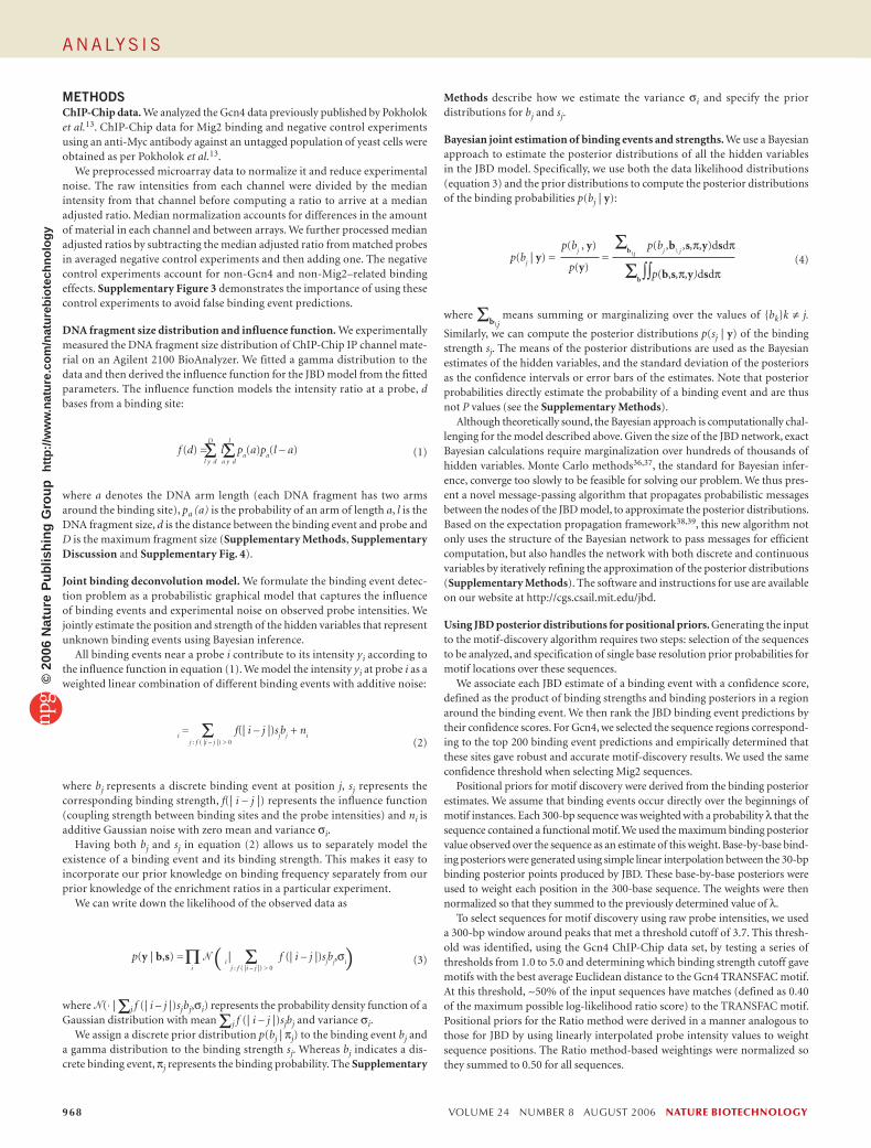
Positional priors bias motif discovery to the correct answer in the absence of informative initialization and in the presence of noise. We incorporated the positional prior into an objective function that is optimized using the Expectation Maximization (EM) algorithm33. EM is a local optimization procedure that is typically restarted from multiple initialization points to reduce its sensitivity to local optima. We investigated the performance of motif discovery on the Gcn4 data set when the motif position weight matrix (PWM) was initialized to background nucleotide frequencies. When we used positional priors, the EM algorithm was insensitive to this uninformative initialization point and produced a motif consistent with the reported specificity34. When positional priors were not used, motif discovery failed to learn a motif consistent with the known specificity. We found that this effect was robust to noise. Information provided by positional priors ren-ders the motif-discovery algorithm resistant to a false-positive input fraction of ~30% (Fig. 4).
DISCUSSIONWe have shown that JBD’s joint learning method is able to reconstruct multiple binding events that appear in raw ChIP-Chip data as a single peak, which is a marked advantage over current approaches. JBD is also able to reconstruct binding events at higher spatial resolution than do competing methods without loss of specificity or sensitiv-ity. JBD may prove to be an important tool for dissecting complex regulatory programs.
JBD accomplishes the above task by probabilistically modeling the noisy data-generation processes with suitable prior probabilities on
binding to enforce a sparseness constraint on binding events. JBD does not use standard deconvolution methods because they would introduce high-frequency spatial noise as a consequence of simply inverting a low-pass filter (the influence function). Simpler nonjoint deconvolution methods such as MPeak fail to handle nearby events, because they rely on heuristics rather than on a generative model to determine the number of binding events that give rise to the observed signal.
Our synthetic results indicate that JBD’s advantages are important at high microarray tiling densities. At high tiling densities, each probe can be influenced by multiple binding events and the effect of a single binding event is spread over more probes. JBD can accurately separate the resulting dense and complicated interference patterns. By analyzing synthetic data ranging over various background noise levels, fragment size distributions and other parameters, we have shown that JBD can increase the effective spatial resolution of data gathered using many different microarray designs and experimental variations.
Finally, we have shown that positional priors at the resolution of tens of bases can accurately recover DNA motifs when a standard method fails, even with very few examples of bound sequence, as in the case of Mig2. Our results further suggest that the use of JBD-derived positional priors reduce the sensitivity of motif-discovery performance to initialization and yield accurate results that are robust to false-positive inputs. In a previous study that profiled Mig2 binding in yeast10, sequences identified as being bound by Mig2 were analyzed using six separate motif-discovery programs, none of which was able to recover a motif consistent with Mig2’s experimentally character-ized specificity35. JBD’s success in guiding motif discovery to the Mig2 motif suggests that it may be useful in searching for other degenerate sequence elements that play critical roles in transcription.
0.6
0.5
0.4
0.3
0.2
0.1E
uclid
ean
dist
ance
to G
cn4
TR
AN
SFA
C m
otif
0 0.1 0.2 0.3 0.4 0.5 0.6 0.7 0.8 0.9 1
Fraction of false positive inputs
Positional prior No positional prior
Figure 4 Positional priors for motif discovery improve robustness to false input DNA sequence regions. To vary the fraction of false-positive input sequences, we partitioned DNA sequence regions containing a potential binding event into positive and negative sets, based on whether they contained a match to the Gcn4 TRANSFAC motif. In each of 87 random trials, sequences with a defined fraction of false-positive examples were randomly sampled from the positive and negative sets. Motif discovery was performed on randomly selected sequence sets, and the mean Euclidean distance of each motif from the TRANSFAC Gcn4 motif was calculated. The plot shows the mean motif distance as a function of the fraction of false-positive sequence examples for the cases in which positional priors are used (squares) or are not used (crosses).
968 VOLUME 24 NUMBER 8 AUGUST 2006 NATURE BIOTECHNOLOGY
METHODSChIP-Chip data. We analyzed the Gcn4 data previously published by Pokholok et al.13. ChIP-Chip data for Mig2 binding and negative control experiments using an anti-Myc antibody against an untagged population of yeast cells were obtained as per Pokholok et al.13.
We preprocessed microarray data to normalize it and reduce experimental noise. The raw intensities from each channel were divided by the median intensity from that channel before computing a ratio to arrive at a median adjusted ratio. Median normalization accounts for differences in the amount of material in each channel and between arrays. We further processed median adjusted ratios by subtracting the median adjusted ratio from matched probes in averaged negative control experiments and then adding one. The negative control experiments account for non-Gcn4 and non-Mig2–related binding effects. Supplementary Figure 3 demonstrates the importance of using these control experiments to avoid false binding event predictions.
DNA fragment size distribution and influence function. We experimentally measured the DNA fragment size distribution of ChIP-Chip IP channel mate-rial on an Agilent 2100 BioAnalyzer. We fitted a gamma distribution to the data and then derived the influence function for the JBD model from the fitted parameters. The influence function models the intensity ratio at a probe, d bases from a binding site:
(1)
where a denotes the DNA arm length (each DNA fragment has two arms around the binding site), pa (a) is the probability of an arm of length a, l is the DNA fragment size, d is the distance between the binding event and probe and D is the maximum fragment size (Supplementary Methods, Supplementary Discussion and Supplementary Fig. 4).
Joint binding deconvolution model. We formulate the binding event detec-tion problem as a probabilistic graphical model that captures the influence of binding events and experimental noise on observed probe intensities. We jointly estimate the position and strength of the hidden variables that represent unknown binding events using Bayesian inference.
All binding events near a probe i contribute to its intensity yi according to the influence function in equation (1). We model the intensity yi at probe i as a weighted linear combination of different binding events with additive noise:
(2)
where bj represents a discrete binding event at position j, sj represents the
corresponding binding strength, f(| i – j |) represents the influence function (coupling strength between binding sites and the probe intensities) and ni is additive Gaussian noise with zero mean and variance σi.
Having both bj and sj in equation (2) allows us to separately model the existence of a binding event and its binding strength. This makes it easy to incorporate our prior knowledge on binding frequency separately from our prior knowledge of the enrichment ratios in a particular experiment.
We can write down the likelihood of the observed data as
(3)
where �(⋅ | Σj f (| i – j |)sj bj,σi) represents the probability density function of a Gaussian distribution with mean Σ j f (| i – j |)sjbj and variance σi.
We assign a discrete prior distribution p(bj | πj) to the binding event bj and
a gamma distribution to the binding strength sj. Whereas bj indicates a dis-
crete binding event, πj represents the binding probability. The Supplementary
Methods describe how we estimate the variance σi and specify the prior
distributions for bj and sj.
Bayesian joint estimation of binding events and strengths. We use a Bayesian approach to estimate the posterior distributions of all the hidden variables in the JBD model. Specifically, we use both the data likelihood distributions (equation 3) and the prior distributions to compute the posterior distributions of the binding probabilities p(bj | y):
(4)
where Σb\j means summing or marginalizing over the values of {bk}k ≠ j.
Similarly, we can compute the posterior distributions p(sj | y) of the binding strength sj. The means of the posterior distributions are used as the Bayesian estimates of the hidden variables, and the standard deviation of the posteriors as the confidence intervals or error bars of the estimates. Note that posterior probabilities directly estimate the probability of a binding event and are thus not P values (see the Supplementary Methods).
Although theoretically sound, the Bayesian approach is computationally chal-lenging for the model described above. Given the size of the JBD network, exact Bayesian calculations require marginalization over hundreds of thousands of hidden variables. Monte Carlo methods36,37, the standard for Bayesian infer-ence, converge too slowly to be feasible for solving our problem. We thus pres-ent a novel message-passing algorithm that propagates probabilistic messages between the nodes of the JBD model, to approximate the posterior distributions. Based on the expectation propagation framework38,39, this new algorithm not only uses the structure of the Bayesian network to pass messages for efficient computation, but also handles the network with both discrete and continuous variables by iteratively refining the approximation of the posterior distributions (Supplementary Methods). The software and instructions for use are available on our website at http://cgs.csail.mit.edu/jbd.
Using JBD posterior distributions for positional priors. Generating the input to the motif-discovery algorithm requires two steps: selection of the sequences to be analyzed, and specification of single base resolution prior probabilities for motif locations over these sequences.
We associate each JBD estimate of a binding event with a confidence score, defined as the product of binding strengths and binding posteriors in a region around the binding event. We then rank the JBD binding event predictions by their confidence scores. For Gcn4, we selected the sequence regions correspond-ing to the top 200 binding event predictions and empirically determined that these sites gave robust and accurate motif-discovery results. We used the same confidence threshold when selecting Mig2 sequences.
Positional priors for motif discovery were derived from the binding posterior estimates. We assume that binding events occur directly over the beginnings of motif instances. Each 300-bp sequence was weighted with a probability λ that the sequence contained a functional motif. We used the maximum binding posterior value observed over the sequence as an estimate of this weight. Base-by-base bind-ing posteriors were generated using simple linear interpolation between the 30-bp binding posterior points produced by JBD. These base-by-base posteriors were used to weight each position in the 300-base sequence. The weights were then normalized so that they summed to the previously determined value of λ.
To select sequences for motif discovery using raw probe intensities, we used a 300-bp window around peaks that met a threshold cutoff of 3.7. This thresh-old was identified, using the Gcn4 ChIP-Chip data set, by testing a series of thresholds from 1.0 to 5.0 and determining which binding strength cutoff gave motifs with the best average Euclidean distance to the Gcn4 TRANSFAC motif. At this threshold, ~50% of the input sequences have matches (defined as 0.40 of the maximum possible log-likelihood ratio score) to the TRANSFAC motif. Positional priors for the Ratio method were derived in a manner analogous to those for JBD by using linearly interpolated probe intensity values to weight sequence positions. The Ratio method-based weightings were normalized so they summed to 0.50 for all sequences.
NATURE BIOTECHNOLOGY VOLUME 24 NUMBER 8 AUGUST 2006 969
Motif discovery. We incorporated positional prior information into a standard motif-discovery algorithm33 in the TAMO package40 to bias the motif search toward regions with high binding posterior estimates. We used the ZOOPS (zero or one occurrences per sequence) probability model outlined as follows:
(5)
Here D corresponds to the set of N input sequences of length M, and the hidden variable Z is a matrix indexed by input sequence and position indicating the start position of functional motifs. The prior probability that a functional motif starts at position j in sequence i is given by γi,j. The ZOOPS model assumes that each sequence contains either zero or one functional motif. We used the EM algorithm described by Bailey and Elkan33 to search for the position weight matrix (PWM) motif model that maximizes the expected log-likelihood of the data given by the above expression.
The positional prior estimates were not only used to guide motif discovery during EM, but also to select initialization points for the PWM before running the algorithm. To search for a motif of width k, we enumerate all k-mers in the input set and count each k-mer’s occurrence, weighting each count by the positional prior value at that location. The top 400 k-mers, by weighted count frequency, are scored by statistical enrichment according to the hypergeometric distribution as described in Harbison et al.10. For trials that did not make use of the positional prior information, no weighting was applied to the counts. The top 20 statisti-cally enriched k-mers were used to initialize the PWM in separate runs of the EM algorithm. For both factors we repeated runs of EM at motif widths of 8, 10 and 15 bp, and the resulting motifs were scored by statistical enrichment. We discarded all motifs with a hypergeometric P > 0.001, and scored the remaining motifs according to their Euclidean distance to the expected motif (see below). For each data set the best match to the expected specificity was reported. We note that for trials using positional prior information the most statistically enriched motif was also the motif that most closely matched the factor’s known specificity. For Gcn4, a motif was available in the TRANSFAC database34. The Mig2 binding specificity has been characterized experimentally35.
We further evaluated the utility of positional priors by examining the robust-ness of our motif-discovery results to false-positive binding events. We used the Gcn4 data set for evaluation, because a sufficient quantity of information was available for performance evaluation. The DNA sequences used to generate our reported Gcn4 motif in Supplementary Figure 2 were partitioned into a positive and negative set, based on whether they contained a match to the Gcn4 TRANSFAC motif. We then generated data sets with a known fraction of false-positive sequences by randomly replacing true-positive sequences in the positive data set with false-positive sequences from the negative data set. During sampling, sequences were weighted by their mean binding strength and binding posterior product to ensure that the data sets were biased toward sequences for which JBD predicts binding. For each data set, motif discovery was performed using either JBD positional priors or with no positional priors. The motif position weight matrix was initialized to background base frequencies for all trials. We calculated the mean Euclidean distance of each motif from the TRANSFAC Gcn4 motif. At each level of false positives, we report the motif distance averaged over six separate randomly selected data sets.
Motif distance calculations. Motifs were scored by their Euclidean distance to an expected motif. For this calculation we determined the alignment of the two motifs that produced the best score. When the reverse complement of a motif yielded a better match, we used the reverse complement. We required a minimum overlap of 6-bp positions. For a motif, M, and an expected motif T, with an overlap of N positions, the score is defined as follows:
The summation over index j is over the four possible bases in the multinomial distribution at a particular position in the PWM.
Note: Supplementary information is available on the Nature Biotechnology website.
ACKNOWLEDGMENTSWe would like to thank Duncan Odom and Laurie Boyer for providing DNA fragment length data for human transcription factors. This work was funded by the National Institutes of Health under grant number GM-069676.
COMPETING INTERESTS STATEMENTThe authors declare competing financial interests (see the Nature Biotechnology website for details).
Published online at http://www.nature.com/naturebiotechnology/Reprints and permissions information is available online at http://npg.nature.com/reprintsandpermissions/
1. Ren, B. et al. Genome-wide location and function of DNA binding proteins. Science 290, 2306–2309 (2000).
2. Lieb, J., Liu, X., Botstein, D. & Brown, P. Promoter-specific binding of Rap1 revealed by genome-wide maps of protein-DNA association. Nat. Genet. 28, 327–324 (2001).
3. Iyer, V. et al. Genomic binding sites of the yeast cell-cycle transcription factors SBF and MBF. Nature 409, 533–538 (2001).
4. Simon, I. et al. Serial regulation of transcriptional regulators in the yeast cell cycle. Cell 106, 697–708 (2001).
5. Lee, T. et al. Transcriptional regulatory networks in Saccharomyces cerevisiae. Science 298, 799–804 (2002).
6. Horak, C. et al. GATA-1 binding sites mapped in the betaglobin locus by using mam-malian ChIP-chip analysis. Proc. Natl. Acad. Sci. USA 99, 2924–2929 (2002).
7. Weinmann, A., Yan, P., Oberley, M., Huang, T. & Farnham, P. Isolating human transcription factor targets by coupling chromatin immunoprecipitation and CpG island microarray analysis. Genes Dev. 16, 235–244 (2002).
8. Li, Z. et al. A global transcriptional regulatory role for c-Myc in Burkitts lymphoma cells. Proc. Natl. Acad. Sci. USA 100, 8164–8169 (2003).
9. Wells, J., Yan, P., Cechvala, M., Huang, T. & Farnham, P. Identification of novel pRb binding sites using CpG microarrays suggests that E2F recruits pRb to specific genomic sites during S phase. Oncogene 22, 1445–1460 (2003).
10. Harbison, C.T. et al. Transcriptional regulatory code of a eukaryotic genome. Nature 431, 99–104 (2004).
11. Cawley, S. et al. Unbiased mapping of transcription factor binding sites along human chromosomes 21 and 22 points to widespread regulation of noncoding RNAs. Cell 116, 499–509 (2004).
12. Robert, F. et al. Global position and recruitment of HATs and HDACs in the yeast genome. Molecular Cell 16, 119–209 (2004).
13. Pokholok, D.K. et al. Genome-wide map of nucleosome acetylation and methylation in yeast. Cell 122, 517–527 (2005).
14. Wyrick, J. et al. Genome-wide distribution of ORC and MCM proteins in S. cere-visiae: high-resolution mapping of replication origins. Science 294, 2357–2360 (2001).
15. Gerton, J. et al. Inaugural article: global mapping of meiotic recombination hotspots and coldspots in the yeast Saccharomyces cerevisiae. Proc. Natl. Acad. Sci. USA 97, 11383–11390 (2000).
16. Bernstein, B.E. et al. Methylation of histone H3 Lys 4 in coding regions of active genes. Proc. Natl. Acad. Sci. USA 99, 8695–8700 (2002).
17. Ng, H., Robert, F., Young, R. & Struhl, K. Regulated recruitment of the ATP-depen-dent chromatin remodeling complex RSC in response to transcriptional repression and activation. Genes Dev. 16, 806–819 (2002).
18. Robyr, D. et al. Microarray deacetylation maps determine genome-wide functions for yeast histone deacetylases. Cell 109, 437–446 (2002).
19. Nagy, P., Cleary, M., Brown, P. & Lieb, J. Genomewide demarcation of RNA poly-merase II transcription units revealed by physical fractionation of chromatin. Proc. Natl. Acad. Sci. USA 100, 6364–6369 (2003).
20. Kurdistani, S.K., Tavazoie, S. & Grunstein, M. Mapping global histone acetylation patterns to gene expression. Cell 117, 721–733 (2004).
21. Bernstein, B.E. et al. Genomic maps and comparative analysis of histone modifica-tions in human and mouse. Cell 120, 169–181 (2005).
22. Yuan, G. et al. Genome-scale identification of nucleosome positions in S. cerevisiae. Science 309, 626–630 (2005).
23. Marion, R.M. et al. Sfp1 is a stress- and nutrient-sensitive regulator of ribosomal protein gene expression. Proc. Natl. Acad. Sci. USA 101, 14315–14322 (2004).
24. Li, X. & Wong, W. Sampling motifs on phylogenetic trees. Proc. Natl. Acad. Sci. USA 102, 9481–9486 (2005).
25. Hartemink, A.J., Gifford, D.K., Jaakkola, T.S. & Young, R.A. Combining location and expression data for principled discovery of genetic regulatory network models. Proceedings of Pacific Symposium on Biocomputing, (Lihue, Hawaii, January 3–7, 2002) 7, 437–449 (2002).
26. Bar-Joseph, Z. et al. Computational discovery of gene modules and regulatory networks. Nat. Biotechnol. 21, 1337–1342 (2003).
970 VOLUME 24 NUMBER 8 AUGUST 2006 NATURE BIOTECHNOLOGY
27. Luscombe, N. et al. Genomic analysis of regulatory network dynamics reveals large topological changes. Nature 431, 308–312 (2004).
28. Buck, M.J., Nobel, A.B. & Lieb, J.D. Chipotle: a user-friendly tool for the analysis of chip-chip data. Genome Biol. 6, R97 (2005).
29. Roberts, C. et al. Signaling and circuitry of multiple MAPK pathways revealed by a matrix of global gene expression profiles. Science 287, 873–880 (2000).
30. Keles, S., Dudoit, S., van der Laan, M. & Cawley, S.E. Multiple testing methods for ChIP-Chip high density oligonucleotide array data. Berkeley Electronic Press (June, 2004). http://www.bepress.com/ucbbiostat/paper147
31. Kim, T.H. et al. A high-resolution map of active promoters in the human genome. Nature 436, 876–880 (2005).
32. Boyer, L.A. et al. Core transcriptional regulatory circuitry in human embryonic stem cells. Cell 122, 947–956 (2005).
33. Bailey, T. & Elkan, C. The value of prior knowledge in discovering motifs with MEME. in Proceedings of the Third International Conference on Intelligent Systems for Molecular Biology, 21–29 (AAAI Press, Menlo Park, CA, 1995).
34. Wingender, E. et al. The TRANSFAC system on gene expression regulation. Nucleic Acids Res. 29, 281–283 (2001).
35. Lutfiyya, L. & Johnston, M. Two zinc-finger-containing repressors are responsible for glucose repression of SUC2 expression. Mol. Cell. Biol. 16, 4790–4797 (1996).
36. Neal, R.M. Probabilistic inference using Markov Chain Monte Carlo methods. Tech. Rep. CRG-TR-93–1, Dept. of Computer Science, University of Toronto (1993).
37. Brooks, S.P. Markov Chain Monte Carlo method and its application. Statistician 47, 69–100 (1998).
38. Minka, T.P. Expectation propagation for approximate Bayesian inference. in Proceedings of Uncertainty in Artificial Intelligence 362–369 (2001). http://research.microsoft.com/~minka/papers/ep/minka-ep-uai.pdf
39. Qi, Y. Extending expectation propagation for graphical models. Ph.D. thesis, MIT (2004). http://www.csail.mit.edu/~alanqi/papers/Qi-PhD-thesis-MIT-04.pdf
40. Gordon, D. B., Nekludova, L., McCallum, S. & Fraenkel, E. Tamo: a flexible, object-oriented framework for analyzing transcriptional regulation using DNA-sequence motifs. Bioinformatics 21, 3164–3165 (2005).