High-resolution limited-angle phase tomography ofdense layered objects using deep neural networksAlexandre Goya,1, Girish Rughooburb, Shuai Lia, Kwabena Arthura, Akintunde I. Akinwandeb,and George Barbastathisa,c

a3D Optics Laboratory, Mechanical Engineering, Massachusetts Institute of Technology, Cambridge, MA 02139; bMicrosystems Technology Laboratories,Electrical Engineering and Computer Science, Massachusetts Institute of Technology, Cambridge, MA 02139; and cBioSystems and bioMechanics (BioSyM)Interdisciplinary Research Group, Singapore-MIT Alliance for Research and Technology (SMART) Centre, Singapore 117543, Singapore

Edited by Terrence J. Sejnowski, Salk Institute for Biological Studies, La Jolla, CA, and approved August 19, 2019 (received for review December 14, 2018)

We present a machine learning-based method for tomographicreconstruction of dense layered objects, with range of projectionangles limited to ±10◦. Whereas previous approaches to phasetomography generally require 2 steps, first to retrieve phaseprojections from intensity projections and then to perform tomo-graphic reconstruction on the retrieved phase projections, in ourwork a physics-informed preprocessor followed by a deep neuralnetwork (DNN) conduct the 3-dimensional reconstruction directlyfrom the intensity projections. We demonstrate this single-stepmethod experimentally in the visible optical domain on a scaled-up integrated circuit phantom. We show that even under con-ditions of highly attenuated photon fluxes a DNN trained onlyon synthetic data can be used to successfully reconstruct physicalsamples disjoint from the synthetic training set. Thus, the needfor producing a large number of physical examples for training isameliorated. The method is generally applicable to tomographywith electromagnetic or other types of radiation at all bands.

deep learning | tomography | imaging through scattering media

Tomography is the quintessential inverse problem. Since theinterior of a 3-dimensional (3D) object is not accessible non-

invasively, the original insight of tomographic approaches was toilluminate through from multiple angles of incidence and thenprocess the resulting projections to reconstruct the interior sliceby slice (1–3). In the simplest case, when diffraction is negligibleand the illumination is collimated, as is generally permissible toassume for X-ray attenuation (4–7) and electron scattering (8–10) in the far field and for features of size ∼1 µm and above,the object’s interior is represented by its Radon transform (11)of line integrals along straight parallel paths. The interior ofthe volume is then reconstructed by use of the Fourier-slicetheorem for the Radon projections. On the other hand, if the X-ray beam is not collimated but spherical, then the slice-by-sliceapproach is no longer applicable and full volumetric reconstruc-tion is required (12, 13). Even when the object is available forobservation from the full 360◦ range of projection angles, theseinstances of tomography are all highly ill-posed because theFourier-slice property results in uneven coverage of the Fourierspace with the high spatial frequencies ending up underrepre-sented. Ill-posedness increases when the angular range is limitedbecause then an entire cone of spatial frequencies goes missingfrom the measurement. Alternatively, in this case, tomosynthesis(14) utilizes sheared (rather than rotated) projections to bringslices from within the interior into focus, but with lower con-trast since emission from the rest of the volume remains asbackground.

Additional challenges occur when the inverse problem ofinterest is to reconstruct in 3D the index of refraction, ratherthan the attenuation. If the object features are large enoughcompared to the wavelength, such that diffraction may still beneglected, and the index variations through the object volumeare relatively small, then each projection may be modeled asa set of Fermat integrals of phase delay along approximatelystraight lines. The phase integrals may be obtained, for exam-

ple, using holographic interferometry (15, 16) or transport ofintensity (17). For smaller-sized features and still assuming weakscattering (first-order Born approximation), the projection inte-grals are instead obtained along curved paths on the surface ofthe Ewald sphere, a method referred to as diffraction tomogra-phy (18, 19). By decoupling the problem into 2 parts, first phaseprojection retrieval, followed by tomography, these approachesenjoy the benefit of using the advanced algorithms in the 2respective research fields. However, there is also the danger thaterrors generated independently during each step may amplifyeach other. Finally, when strong scattering may no longer beneglected, all 2-step approaches become questionable becausethe interpretation of the first step as line integrals is no longervalid.

Generally, ill-posed inverse problems are solved by regularizedoptimization. If f is the object and g the measurement, then theobject estimate f is obtained as (20, 21)

f = argminf

{‖Hf − g‖2 +αΦ(f )

}. [1]

Here, H is the forward operator relating the measurement tothe object, Φ is the regularizer expressing prior knowledge aboutthe object, and α is the regularization parameter controlling thecompetition between the 2 terms. The prior may be thought ofas rejecting solutions to the inverse problem that are known toviolate known properties of the class of objects being imaged;for example, if the class where f belongs is known to have sharpedges, then the regularizer should be applying a high penaltyto blurry solutions f . Thus, the inherent uncertainty due toill-posedness is reduced. Sparsity-promoting compressive priors(22–25) found some of their first successes in tomographic recon-struction (26, 27). Compressive sensing is directly implementedthrough a proximal gradient solution to Eq. 1 if a set of basis

Significance

We demonstrate that it is possible to use deep neural net-works to produce tomographic reconstructions of dense lay-ered objects with small illumination angle as low as 10◦. It isalso shown that a DNN trained on synthetic data can gener-alize well to and produce reconstructions from experimentalmeasurements. This work has application in the field of X-raytomography for the inspection of integrated circuits and othermaterials studies.

Author contributions: A.I.A. and G.B. designed research; A.G. performed research; G.R.,S.L., and K.A. contributed new reagents/analytic tools; A.G. analyzed data; and A.G., G.R.,and G.B. wrote the paper.y

The authors declare no conflict of interest.y

This article is a PNAS Direct Submission.y

This open access article is distributed under Creative Commons Attribution-NonCommercial-NoDerivatives License 4.0 (CC BY-NC-ND).y1 To whom correspondence may be addressed. Email: agoy@goyman.com.y

First published September 16, 2019.

19848–19856 | PNAS | October 1, 2019 | vol. 116 | no. 40 www.pnas.org/cgi/doi/10.1073/pnas.1821378116

Dow

nloa

ded

by g

uest

on

Nov

embe

r 19

, 202

1

ENG

INEE

RIN

G

functions where the object class is sparse is a priori known. Alter-natively, if a database of representative objects is available, thenthese examples may be used to learn the optimal set of basisfunctions as a dictionary (28, 29).

Rapid recent developments in the field of machine learn-ing, and deep neural networks (30) (DNNs) in particular, haveprovided an additional set of tools and insights for inverse prob-lems. It may be shown (31, 32) that recurrent or unfoldedmultistage DNN architectures are formally equivalent to the iter-ative solution to the inverse problem in Eq. 1 where the priorΦ need no longer be known or depend on sparsity; instead,examples guide the discovery of the prior through the DNNtraining process. Simpler learning architectures, where g is fedto the DNN directly or after first passing through a preproces-sor, have been used for retrieval of phase from intensity (33–36);3D holographic reconstruction (37–39); superresolution photog-raphy (40–42) and microscopy (43); imaging through scatter(44–47); and imaging under extremely low light conditions in the3 contexts computational ghost imaging (48), consumer-cameraphotography (49), and phase retrieval (50).

Multistage DNN architectures have been shown to yield high-quality reconstructions in numerous Radon tomography con-figurations (32, 51–56). Recently, Nguyen et al. (57) used theinverse Radon transform for optical tomography with a single-stage DNN intended to partially correct for the assumption ofline integrals breaking down.

In this paper, we apply a Fourier-based beam propagationmethod (BPM) (58) as a preprocessing step immune from anyRadon assumptions. The strongly scattering object is illuminatedby a parallel beam under a limited angular range of 20◦, i.e.,±10◦ from the reference axis. Unlike the earlier works on refrac-tive index tomography referenced above, we do not perform aphase retrieval step; rather, the intensity measurements are pre-processed to produce directly an initial crude 3D guess of theobject’s interior. This crude guess is then fed to our machine-learning algorithm. The preprocessing step is necessary because,even if we did convert intensity to phase, the results would notbe interpretable as line integrals under our experimental con-ditions. Moreover, by merging phase retrieval and tomographyinto a single step, our algorithm becomes less sensitive to erroraccrual.

Large datasets, typically consisting of more than 5,000 exam-ples, are generally required for DNN training. That is feasiblein many cases through spatial light modulators (33, 57). How-ever, in many cases of interest spatial light modulators haveinsufficient space-bandwidth product or are unavailable (e.g.,in X-rays); and alternatives to generate physical specimens areexpensive or restricted due to proprietary processes. Instead,our approach is to train the DNN on purely synthetic datawith the rigorous BPM forward model and then use a physicaltest specimen (phantom) to test the reconstruction quality withwell-calibrated ground truth in experiments.

We chose to design our phantom as emulating the 3D geom-etry of integrated circuits (ICs). These would normally beinspected with X-rays, so we scaled up the feature dimensionsin the phantom for visible wavelengths. The advantage of thischoice is that IC layouts provide strong geometrical priors, e.g.,Manhattan geometries, and our phantom also exhibited largespatial gradients and refractive index contrast to strengthen scat-tering. Thus, our methodology is directly applicable to all casesof tomography at optical wavelengths, e.g., 3D-printed speci-men characterization and identification and biological studiesin cells and tissue with moderate scattering properties. In eachcase, testing the ground truth would require the fabricationor the accurate simulation of different phantoms meeting thecorresponding priors.

There is also value in the study of emulating X-ray inspec-tion of ICs at visible wavelengths, as extensive outsourcing

by the IC industry has created a growing concern that theICs delivered to the customer may not match the expecteddesign and that malicious features may have been added (59).However, in our emulation the phase contrast of the featuresagainst the background and the Fresnel number are both higherthan typical corresponding IC configurations even at soft X-raywavelengths.

One advantage of deep learning for inverse problems is speed.Solving [1] separately for each instance of g is computation-ally intensive, and training a DNN is even more so. This isbecause both operations are iterative, and the latter is run onlarge datasets. On the other hand, once the DNN has learnedthe inverse map from the preprocessed version of g to f , thecomputations are feedforward only. For example, the IC lay-out priors we exploit here could, in principle, also be learned bydictionaries—but, under strong scattering conditions, the latterwould require iterative optimization of Eq. 1 with the forwardoperator H itself consisting of an expensive computational pro-cedure in each iteration. In our approach, the preprocessingperformed prior to the DNN is the most time-consuming opera-tion, and therefore we aim at simplifying the preprocessing stepas much as we can, i.e., tolerate a crude approximation, andleave it to the DNN to correct it. In our case, the executiontime is 51 s (out of which only 300 ms are taken by the DNN,with the rest being the preprocessor), while learning tomography(60, 61), which is based on a similar gradient descent algorithm,takes 212 s and yields inferior reconstructions (see Fig. 4 forthis, and see Materials and Methods for the computing hardwareimplementation).

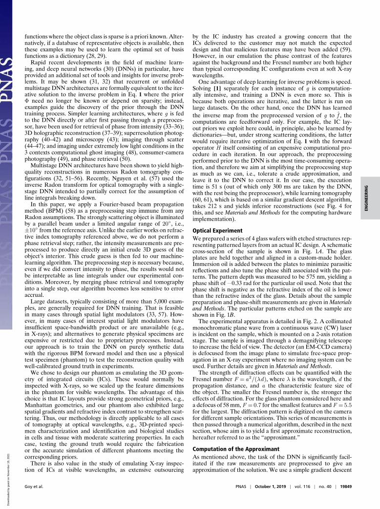
Optical ExperimentWe prepared a series of 4 glass wafers with etched structures rep-resenting patterned layers from an actual IC design. A schematiccross-section of the sample is shown in Fig. 1A. The glassplates are held together and aligned in a custom-made holder.Immersion oil is added between the plates to minimize parasiticreflections and also tune the phase shift associated with the pat-terns. The pattern depth was measured to be 575 nm, yielding aphase shift of −0.33 rad for the particular oil used. Note that thephase shift is negative as the refractive index of the oil is lowerthan the refractive index of the glass. Details about the samplepreparation and phase-shift measurements are given in Materialsand Methods. The particular patterns etched on the sample areshown in Fig. 1B.

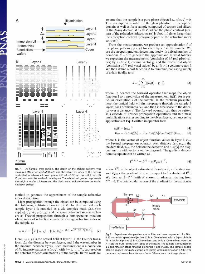
The experimental apparatus is detailed in Fig. 2. A collimatedmonochromatic plane wave from a continuous wave (CW) laseris incident on the sample, which is mounted on a 2-axis rotationstage. The sample is imaged through a demagnifying telescopeto increase the field of view. The detector (an EM-CCD camera)is defocused from the image plane to simulate free-space prop-agation in an X-ray experiment where no imaging system can beused. Further details are given in Materials and Methods.

The strength of diffraction effects can be quantified with theFresnel number F = a2/(λd), where λ is the wavelength, d thepropagation distance, and a the characteristic feature size ofthe object. The smaller the Fresnel number is, the stronger theeffects of diffraction. For the glass phantom considered here anda defocus of 58 mm, F = 0.7 for the smallest features and F = 5.5for the largest. The diffraction pattern is digitized on the camerafor different sample orientations. This series of measurements isthen passed through a numerical algorithm, described in the nextsection, whose aim is to yield a first approximate reconstruction,hereafter referred to as the “approximant.”

Computation of the ApproximantAs mentioned above, the task of the DNN is significantly facil-itated if the raw measurements are preprocessed to give anapproximation of the solution. We use a simple gradient descent

Goy et al. PNAS | October 1, 2019 | vol. 116 | no. 40 | 19849

Dow

nloa

ded

by g

uest

on

Nov

embe

r 19

, 202

1

B

Layer 1

Layer 2

Layer 3

Layer 4

Cover0.5mm thickfused silicawafers

Immersion oil

Layer 4

Layer 2

Layer 3

Layer 1

10mm

Illumination

Δz

A

Fig. 1. (A) Sample cross-section. The depth of the etched patterns wasmeasured (Materials and Methods) and the refractive index of the oil wascontrolled to achieve a known phase shift of −0.32 rad. ∆z = 0.5 mm. (B)IC patterns used for each of the 4 layers. The white background representsthe original wafer thickness and the black areas indicate where the waferhas been etched.

method to generate the approximant of the sample refractiveindex distribution.

Light propagation through the object can be computed usingthe following split-step Fourier BPM. In this method eachsample layer l is modeled as a 2D complex mask fl(x , y) =exp[αl(x , y) + jϕl(x , y)] and the space between 2 successive lay-ers as Fresnel propagation through a homogeneous mediumwhose index of refraction equals the average refractive index ofthe sample, as

ul =F−1{F {ul−1fl−1}(kx , ky)e−j(k−

√k2−k2

x −k2y )∆z

}. [2]

Here, ul(x , y) is the optical field at layer l , F the Fourier trans-form, ∆z the distance between layers, and k the wavenumber inthe medium between layers. Each measurement is a collectionof Nv intensity patterns gi(x , y), with i = 1, . . . ,Nv , captured onthe detector for each orientation i of the sample. In this work, we

assume that the sample is a pure phase object; i.e., α(x , y) = 0.This assumption is valid for the glass phantom in the opticaldomain as well as for a sample composed of copper and siliconin the X-ray domain at 17 keV, where the phase contrast (realpart of the refractive index contrast) is about 10 times larger thanthe absorption contrast (imaginary part of the refractive indexcontrast).

From the measurements, we produce an approximation f ofthe phase pattern ϕl(x , y) for each layer l in the sample. Weuse the steepest gradient descent method with a fixed number ofiterations K = 8 to generate the approximant. In what follows,we represent the measurements (consisting of M real pixel val-ues) by a (M × 1) column vector gi and the discretized object(consisting of N real voxel values) by a (N × 1) column vector f.We then define a cost function J to minimize, consisting simplyof a data fidelity term

J =1

2

Nv∑i=1

‖Hi(f)− gi‖22, [3]

where Hi denotes the forward operator that maps the objectfunction f to a prediction of the measurement Hi(f), for a par-ticular orientation i of the sample. In the problem presentedhere, the optical field will first propagate through the sample Llayers, each of thickness ∆z , and then in free space to the detec-tor over a distance d . The forward operator can thus be writtenas a cascade of Fresnel propagation operations and thin maskmultiplications corresponding to the object layers, i.e., successiveapplications of Eq. 2 written in operator form

Hi(f) = |udet|2 [4]udet =Fddiag[fL] . . .F∆zdiag[f2]F∆zdiag[f1]uinc,i , [5]

where fl is the vector of object function values in layer l , F∆z

the Fresnel propagation operator over distance ∆z , uinc,i theincident field, udet the field on the detector, and diag[v] the diag-onal matrix with vector v on the diagonal. The gradient descentiterative update can be written as

f(k+1) = f(k)− s(∇f(k)J )T , [6]

where f(k) is the object estimate at iteration k , s the step size,and ∇f(k)J the gradient of J with respect to f evaluated at f(k).We then set f = f(K) with K chosen in advance, starting fromf(0) = 0. The detailed derivation of the gradient for the particular

He-Ne laser

EM-CCD

L3 L4

L1L2

F1

Imageplane

Sample

A1

x

y z

Fig. 2. Experimental apparatus: spatial filter and beam expander. L1 is 10×,0.25 numerical aperture objective; L2 is a 100-mm lens, with a 5-µm pinholeF1 in the focal plane; L3 is a 200-mm lens; and L4 is a 100-mm lens. ApertureA1 cuts the outer diffraction lobes of the beam. The sample is mounted ona 2-axis rotation stage rotating along the x and y axes. The sample middleplane is imaged using a telescope lens system with magnification 0.50×. Thecamera is defocused by a distance ∆z = 58 mm from the image plane.

19850 | www.pnas.org/cgi/doi/10.1073/pnas.1821378116 Goy et al.

Dow

nloa

ded

by g

uest

on

Nov

embe

r 19

, 202

1

ENG

INEE

RIN

G

200

600

(cou

nts)

A B

-0.25

0.15

(rad

)

Fig. 3. (A) Examples of experimental intensity measurement for thesample orientation (θx =−10◦, θy = 0◦). (B) Phase approximant for IClayer 1 obtained from the collection of 22 intensity patterns at dif-ferent orientations (θx =−10◦,−8◦, . . . , +10◦, θy = 0◦) and (θx = 0◦, θy =

−10◦,−8◦, . . . , +10◦).

model in Eqs. 4 and 5 is given after the conclusion in the Deriva-tion of the Gradient section. In Fig. 3, we give an example of 1experimental intensity measurement (g1) taken from the seriesof tomographic projections and the corresponding approximantf(8) obtained from the whole series using Eq. 6.

DNN Architecture and TrainingWe use a DNN to map the approximant to the final recon-struction f. The DNN is a convolutional neural network with aDenseNet architecture (62). The implementation is the same asthe DNN used in ref. 45 except that the number of dense blockswas reduced to 3 in both the encoder and the decoder, as weempirically observed that using more dense blocks did not resultin a significant improvement of the results. We produce a totalof 5,500 synthetic sets of measurements obtained by simulatingthe optical apparatus with the beam propagation method in Eq.2. The synthetic measurements were subject to simulated shotnoise and read noise equivalent to the noise levels found in theexperiment. The shot noise was accounted for by converting thesimulated measurement pixel intensities I expressed in averagephoton count per pixel per integration period of the detector tointeger numbers of photons N following Poisson statistics. Theactual optical power on the camera was measured with a powermeter and converted to an average photon flux per detector pixel.Read noise following Gaussian statistics was subsequently added.The parameters (variance and average) of the noise were mea-sured from a series of dark frames from the camera taken withthe same gain (EM gain of 1) and integration time (2 ms) as theexperimental measurements.

From each set of measurements, we produce a multilayerapproximant using the gradient descent in Eq. 6. The examplesare split in a training set of 5,000 examples, a validation set of450 examples, and a test set of 50 examples. Each set of measure-ments (1 example) comprises 22 views corresponding to differentorientations of the sample. The DNN is then trained to mapthe approximant to the ground truth used for the simulation.Each layer of the sample is assigned to a different channel inthe DNN. We use the negative Pearson correlation coefficient(NPCC =−PCC) as loss function and train in 20 epochs with abatch size of 16 examples. For 2 images A and B , the PCC isdefined as

PCC(A,B) =

∑i(Ai − A)(Bi − B)√∑

i(Ai − A)2∑

i(Bi − B)2

, [7]

The PCC (and therefore the NPCC too) is agnostic to scale andoffset; i.e., PCC(aA+ b, cB + d) = PCC(A,B) for a, b, c, d ∈R. As a consequence, the DNN, which is trained by minimizingthe NPCC, may apply some offset and scaling to the reconstruc-tion. These parameters are not easily predictable; however, for agiven DNN they are constant once training is complete, which

allows us to correct the reconstructions. Offset and scale areobtained by least-squares linear regression between the DNNoutput and the ground truth from the synthetic test set examples(not including the experimental example).

ResultsThe method described in the previous sections was applied tothe glass phantom shown in Fig. 1B. The synthetic measure-ments were subject to Poisson noise resulting from 103 photonflux per detector pixel, equal to the experimental photon flux,and an additive Gaussian noise with a SD of 13 counts. ForDNN training, we compared 2 sets of approximants, obtainedwith K = 1 and K = 8 with and without total variation (TV) reg-ularization. In the case K = 1, the regularization parameter αwas set to 0.1 (step size 0.1). We chose a smaller value of 0.04for the case K = 8 (step size 0.05) because the proximal opera-tor corresponding to the regularizer is applied at each iterationand its effect tends to accumulate. In the case K = 8, the partic-ular choice for the number of iterations is an empirical trade-offbetween computation time and accuracy. The same optimizationparameters (step size and number of iterations) were used tocompute the approximant of the IC phantom, and the result foreach layer is shown in Fig. 4 E–H for K = 1 and Fig. 4 I–L forK = 8. The DNN reconstruction results are summarized in Fig. 4M–P (K = 1) and Fig. 4 Q–T (K = 8). The approximant and theDNN reconstruction represent the phase modulation imposedby each layer in the sample. The absolute phase carries no use-ful information; therefore we are free to offset the reconstructedphase by an arbitrary constant. In the DNN reconstructions inFig. 4 I–L, the IC patterns (where the phase shift actually occurs)are typically reconstructed with 0 phase due to the rectified linearunits (which project all negative values to 0) at the output layerof the DNN. We reassign the phase of the pattern to the nomi-nal phase of −0.33 rad so that it can be visually compared to theground truths in Fig. 4 M–P. An alternate approach leading tovery similar results is to assign a 0 phase to the background.

The DNN reconstructions can be compared to those obtainedusing learning tomography (LT), a previously demonstratedoptical tomography technique (60, 61) based on proximal opti-mization (FISTA) (63) with TV regularization (64). The role ofthe TV regularizer is to favor piecewise constant solutions whilepreserving sharp edges, which is especially well suited for IC pat-terns. LT was initially designed for holographic measurementsand was modified here to work on intensity measurements bycomputing the gradient for the data fidelity term in Eq. 3. Theessential difference in the LT optimization is that a TV filterplaying the role of a proximal operator is applied at each iter-ation on the current solution. The LT reconstructions for theexperimental dataset are shown in Fig. 4 A–D. These particu-lar reconstructions were obtained after 30 iterations of gradientdescent, a step size of 0.05, a regularization parameter α= 0.04,and 20 iterations for the TV regularizer at each step. The com-putation time of the f(8) approximant is 51 s for K = 8 (noregularization) and 6 s for K = 1, including 570 ms for the DNNvs. 212 s for LT on the same processor (see Materials and Methodsfor hardware details).

In Table 1, we summarize the values of the PCC, which weuse to quantify the quality of the reconstructions. The values aregiven for reconstructions on the synthetic test set (50 examples)and also the reconstruction of the single experimental example.Because the reconstruction quality turns out to depend stronglyon the particular layer, we display the value for each of the 4layers separately. As may be expected, the values for the LT arehigher (better reconstructions) than those for the approximantas LT was run for 30 iterations vs. 8 for the approximant and thatthe latter was not regularized. The DNN reconstructions appearto be the best according to the PCC metric, which shows that,even while starting from a poor approximation, the DNN was

Goy et al. PNAS | October 1, 2019 | vol. 116 | no. 40 | 19851

Dow

nloa

ded

by g

uest

on

Nov

embe

r 19

, 202

1

DN

N r

econ

str.,

K=

1

-0.33

0.05

(rad)

Layer 1 Layer 2 Layer 3 Layer 4

App

roxi

man

t, K

=1

Des

ign

-0.33

0.05

(rad)

A B C D

E F G H

I LJ K

Reg

ular

ized

GD

U XV W

-0.25

0.15

(rad)

-0.1

0.1

(rad)

App

roxi

man

t, K

=8

DN

N r

econ

str.,

K=

8

-0.33

0.05

(rad)

M N O P

Q TR S

-0.25

0.15

(rad)

Fig. 4. (A–D) Proximal gradient descent with TV regularization, K = 30 iterations, for each layer 1 to 4. (E–H) Approximants generated from the experimen-tal measurements with K = 1. (I–L) Approximants generated from the experimental measurements with K = 8. (M–P) Reconstructions from the DNN of eachapproximant E–H, respectively. (Q–T) Reconstructions from the DNN of each approximant I–L, respectively. (U–X) Idealized ground truth obtained from thesample specifications for layers 1 to 4. Note that the color bar range covers more than the range of the data, so there is no saturation effect on the images.

able to outperform LT. Note that a direct comparison betweenthe performance of the DNN on the synthetic data and that onthe experimental example is not fair because the ground truthis not known in the experiment. The ground truth used for the

experimental example is an idealization from the design param-eters used to fabricate the sample. We also indicate the valuesfor reconstructions based on the regularized approximant (usingthe same regularization parameters as in the LT algorithm).

19852 | www.pnas.org/cgi/doi/10.1073/pnas.1821378116 Goy et al.

Dow

nloa

ded

by g

uest

on

Nov

embe

r 19

, 202

1

ENG

INEE

RIN

G

Table 1. PCC, expressed in percentage (i.e., PCC × 100), of the reconstructions in the test setwith respect to the ground truths for the approximant (not regularized) and the DNNreconstructions, labeled “DNN,” obtained from the unregularized approximant

Approximant DNN DNN reg. LT

K Layer Simul. Exp. Simul. Exp. Simul. Exp. Simul. Exp.

1 1 62 ± 7 48 99 ± 0.3 80 99 ± 0.4 72 91 ± 2 651 2 43 ± 5 22 97 ± 1 56 96 ± 1 45 79 ± 7 371 3 49 ± 9 41 99 ± 0.4 77 94 ± 5 76 89 ± 3 621 4 24 ± 7 7 95 ± 1 38 92 ± 2 42 76 ± 7 278 1 75 ± 63 63 100 ± 0.2 75 100 ± 0.1 76 — —8 2 57 ± 6.5 31 98 ± 0.7 44 99 ± 0.4 45 — —8 3 62 ± 6.5 52 99 ± 0.3 80 99 ± 0.3 79 — —8 4 41 ± 8.1 12 96 ± 0.8 48 98 ± 0.6 43 — —

We show the 2 cases K = 1 and K = 8 for the approximant calculation. The LT solution is obtained with K = 30and is indicated on the right. The values for the DNN trained with regularized approximants are labeled “DNNreg.” The uncertainty values indicated correspond to the SD over the 50 examples of the test set. For each case,the values for the synthetic (simulated) and experimental examples are indicated in separated columns “Simul.”and “Exp.,” respectively. No uncertainty is given for the experimental case as it contains only 1 example.

In terms of PCC, there is no significant difference from theunregularized case.

The reconstructions based on regularized approximants areshown in Fig. 5. By comparing these images with the unregular-ized reconstructions shown in Fig. 4, and also by considering thevalue of the PCC in Table 1, we conclude that the regularizationhas little effect, especially on the experimental reconstructions.Moreover, the TV regularization may not operate as a favorablepreconditioner for the DNN. The choice of the TV operator as aregularizer is arbitrary and only based on our assumption thatthe solution should be piecewise constant. In fact, because ofthe small angle range, the approximants for the different phan-tom layers are quite similar to each other and the regularizationmay cancel information that the DNN could use to discrimi-nate between them. Layers 3 and 4 can be said to look visuallybetter with the regularized approximant, but the situation isreversed for layers 1 and 2. Iterating more, i.e., using K = 8 vs.K = 1, yields slightly better results as can be expected intuitively,but the improvement is quite minute considering the increasedcomputation time required to perform 7 more iterations.

In the regularized case K = 1 only we observed instability inthe behavior of the DNN for the regularized approximants. Forbipolar input (approximant containing both positive and nega-tive values), one of the phantom layers (layer 3) would always bereconstructed to null values. As we are using a rectified linearunit as an activation function, this means that the output of onelayer within the network displays only negative values. By offset-ting the input to the DNN (approximant) so that all values arepositive we were able to remove the problem (reconstructions ofFig. 5 I–L). For the regularized K = 1 case where this behaviorwas observed, the difference between approximant layers is thesmallest; i.e., the failure may be due to the regularizer washingout the differences.

So far, we have reconstructed the phase shift distributionϕ(x , y) associated to each layer. In fact, it is possible, with thesame method, to infer the refractive index n(x , y) of the sam-ple. For a given layer, the refractive index is simply given byn(x , y) =ϕ(x , y)/(k∆z ), where ∆z is the thickness of the layer.If the layer thicknesses are not known, one would instead slicethe object into layers at finer spacing to meet the applicableNyquist criterion.

ConclusionIn this paper, we have demonstrated through an emulated X-rayexperiment that DNNs can be used to improve the reconstruc-tion of IC layouts from tomographic intensity measurements

acquired within an angle range of ±10◦ along each lateralaxis. The approximant obtained after 1 or several iterationsof the steepest gradient method does not provide a recon-struction of sufficient quality for the purpose of IC integrityassessment. The DNN, however, exploits the strong prior con-tained in the object geometry and yields reconstructions that aresignificantly improved over the approximant. One of the mainmotivations for using DNN is indeed the speed of execution;therefore, we want to limit any unnecessary preprocessing. Infact, trying to improve the quality of the approximant by sim-ply iterating more the gradient descent does not yield significantimprovement.

One significant challenge for the method we demonstrated isto provide a proper training set for the DNN. In the case ofICs, the training set is simply given by the many real layoutsthat are available. For more generic objects, a problem needsfirst to be formulated to clearly define the class of object onwhich the training will be performed. This is, however, the casein general for problem solving that involves DNNs. What hasbeen shown here is the compelling improvement that DNN canbring to a phase tomography problem when the class of objectis known.

More generally, there is a trade-off between the specificity ofthe required priors and the “difficulty” of an inverse problem—measured as degree of ill-posedness, e.g., the ratio of largest tosmallest eigenvalue in a linearized representation of the forwardoperator. The problem we addressed here is severely ill-poseddue to the presence of strong scattering within the object and thelimited range and number of angular measurements we allowedourselves to collect. Therefore, the rather restricted nature ofICs as a class prior is justified; while, at the same time, ourapproach is addressing an indisputably important practical prob-lem. Detailed determination of the relationship between thedegree of ill-posedness and the complexity of the object classprior would be a worthwhile topic for future work.

Derivation of the Gradient. This derivation follows a path similarto the derivation given in ref. 61. We start from Eq. 3:

J =1

2

Nv∑i=1

‖Hi(f)− gi‖22 [8]

=1

2

Nv∑i=1

(Hi(f)THi(f)− 2Hi(f)Tgi + gT

i gi

). [9]

Goy et al. PNAS | October 1, 2019 | vol. 116 | no. 40 | 19853

Dow

nloa

ded

by g

uest

on

Nov

embe

r 19

, 202

1

DN

N r

econ

str.,

K=

1

-0.33

0.05

(rad)

Layer 1 Layer 2 Layer 3 Layer 4A

ppro

xim

ant,

K=

1 A B C D

E F G H

I LJ K

-0.1

0.1

(rad)

App

roxi

man

t, K

=8

DN

N r

econ

str.,

K=

8

-0.33

0.05

(rad)

M N O P

-0.25

0.15

(rad)

Fig. 5. (A–D) Approximants generated from the experimental measurements with K = 1 and TV regularization with α= 0.1. (E–H) Approximants obtainedwith K = 8 and TV regularization with α= 0.04. (I–L) Reconstructions from the DNN of each approximant A–D, respectively. (M–P) Reconstructions from theDNN of each approximant E–H, respectively.

The gradient of J is defined as

∇fJ =

[∂J

∂ϕ1, . . . ,

∂J

∂ϕN,∂J

∂α1, . . . ,

∂J

∂αN

]f(k)

, [10]

where the object function is defined as f = exp[jϕ−α], withϕ representing the phase delay and α the absorption. In whatfollows we denote the gradient by ∇ for notational simplicity.We take the gradient of Eq. 9 and, by linearity of the deriva-tion operation and denoting Hi(f) by Hi = (H1, . . . ,HM )T ,we get

∇J =1

2

Nv∑i=1

[∇(HT

i Hi)− 2∇(HTi gi)

]. [11]

The term ∇(gTi gi) is absent because measurements gi do not

depend on the estimate f. Then, by the definition

∇H =

∂H1∂ϕ1

. . . ∂H1∂ϕN

∂H1∂α1

. . . ∂H1∂αN

. . .∂HM∂ϕ1

. . . ∂HM∂ϕN

∂HM∂α1

. . . ∂HM∂αN

, [12]

we get

∇J =

Nv∑i=1

[HT

i ∇Hi − gTi ∇Hi

][13]

=

Nv∑i=1

[rTi ∇Hi

], [14]

19854 | www.pnas.org/cgi/doi/10.1073/pnas.1821378116 Goy et al.

Dow

nloa

ded

by g

uest

on

Nov

embe

r 19

, 202

1

ENG

INEE

RIN

G

where ri is the residual defined as ri = Hi − gi . Finally, we getthe expression required in Eq. 6:

(∇J )T =

Nv∑i=1

(∇Hi)T ri . [15]

In Eq. 15, (∇Hi)T is a matrix of size (2N ×M ) that is too large

to be computed directly. Instead, we use a routine, describedbelow, to calculate the vector (∇Hi)

T ri directly. We remind thereader of Eqs. 4 and 5 that describe the forward model wherewe drop the index i to simplify the notation as the expressionassumes the same form for each sample orientation:

H = |udet|2 [16]

udet =Fddiag[fL] . . .F∆zdiag[f2]F∆zdiag[f1]uinc. [17]

This forward operator allows for a convenient computationof the gradient by using a backpropagation scheme. We firstcalculate the gradient of Eq. 16,

∇H =∇|udet|2 [18]

=∇(diag[u∗det]udet) [19]

= diag[udet]∇u∗det + diag[u∗det]∇udet [20]

= 2<{diag[u∗det]∇udet}, [21]

where the asterisk represents the complex conjugate. Thus,

(∇H)†r = 2<{

(∇udet)†r′}

, [22]

where the dagger represents the Hermitian transpose and wehave defined r′= diag[udet]r. Because it is not practical to com-pute the matrix (∇udet)

† due to its size, we use a recursivescheme to compute (∇udet)

†r′ directly. For that, we rewrite Eq.17 as a recursive relationship for the optical field ul just afterlayer l :

u1 = diag[f1]uinc [23]ul = diag[fl ]F∆zul−1 [24]

udet =FduL. [25]

The optical field u is thus known everywhere for a given objectfunction f. We then propagate the residual r′ backward throughthe sample by using the same propagation relationships:

r′L =F †d r′ [26]

r′l−1 =F †∆zdiag[fl ]†r′l . [27]

Note that the Fresnel operator is unitary; i.e., F †=F−1. We takethe gradient of Eqs. 23–25:

∇u1 = diag[uinc]∇f1 [28]∇ul = diag[F∆zul−1]∇fl + diag[fl ]F∆z∇ul−1 [29]∇udet =Fd∇uL. [30]

We then take the Hermitian transpose and multiply by theresidual; we get

(∇u1)†r′1 = (∇f1)†diag[uinc]†r′1 [31]

(∇ul)†r′l = (∇fl)

†diag[F∆zul−1]†r′l +

+ (∇ul−1)†F †∆zdiag[fl ]†r′l [32]

(∇udet)†r′= (∇uL)†F †d r′. [33]

We simplify the equations above by making use of Eqs. 24 and25,

(∇u1)†r′1 = (∇f1)†diag[uinc]†r′1 [34]

(∇ul)†r′l = (∇ul−1)†r′l−1 + (∇fl)

†diag[F∆zul−1]†r′l [35]

(∇udet)†r′= (∇uL)†r′L, [36]

which gives us a recursive relationship to calculate the gradi-ent of the field at each layer. Note that (∇fl)† is a matrixof size 2N ×M whose entries are nonzeros only for thediagonal entries corresponding to layer l because fi dependsonly on αi and ϕi . In practice, (∇udet)

†r′ can be builtlayer by layer by stacking the second term of the right-hand side of Eq. 35 which reads, for pure phase objects(α= 0),

(∇fl)†diag[F∆zul−1]†r′l =−jdiag[e−jϕl ]diag[F∆zul−1]†r′l

[37]

=−jdiag[e−jϕl ]diag[e jϕl ]diag[u∗l ]r′l [38]

=−jdiag[u∗l ]r′l , [39]

where we have used Eq. 24. Finally, according to Eq. 22, weobtain layer l of (∇H)†r,

(∇H)†r|layer l = 2={

diag[u∗l ]r′l}

, [40]

where = denotes the imaginary part.

Materials and MethodsThe experimental apparatus is shown in Fig. 2A. The light source is a CWHe-Ne laser at 632.8 nm that is spatially filtered, expanded, and collimatedinto a quasi-plane wave with an Airy disk intensity profile of 33 mm indiameter. The sample is mounted on a 2-axis rotation stage rotating alongthe x and y axes. The sample middle plane is imaged using a demagni-fying telescope (×0.50) lens system to enhance the effect of diffractionand increase the field of view on the detector. The detector is an EM-CCD(QImaging Rolera EM-C2) with a 1,004 × 1,002 array of 8× 8-µm pixels. Tosimulate the diffraction occurring in an X-ray measurement, the detector isdefocused by a distance ∆z = 58 mm from the image plane, which corre-sponds to Fresnel numbers ranging from 0.7 to 5.5 for the different objectfeatures.

The sample corresponds to a 104× scale-up of a real IC design. The orig-inal IC comprises 13 layers, including the doped layers. We kept only layers5 to 8 from the original design (relabeled here 1 to 4) shown in Fig. 2Cthat contain copper patterns that would induce a significant phase delay inthe X-ray regime. The 4 glass plates corresponding to the IC layers were cutin a 500-µm-thick fused silica wafer and 575± 5-nm deep patterns (mea-sured after fabrication with a Bruker DekTak XT stylus profilometer) wereobtained by wet etching. To control the phase contrast and reduce para-sitic reflections between the layers, we used an immersion oil (Fig. 2B) witha refractive index nD = 1.400± 0.0002 at 25 ◦C from Cargille-Sacher Lab-oratories. According to the manufacturer, the refractive index of the oil isnoil = 1.4005± 0.0002 at 632.8 nm and 20 ◦C. The refractive index of fusedsilica is nglass = 1.457 at 632.8 nm and 20 ◦C (65), which gives a contrast of∆n = 0.0565± 0.0005. The corresponding phase shift for a single pattern isthen ∆ϕ= kd∆n = 0.323± 0.006 rad.

The sample layers are fabricated on double-sided polished 150-mm-diameter and 500-µm-thick fused silica wafers. A 1-µm-thick positive toneresist (Megaposit SPR700) is spin coated at 3,500 rpm on both sides of thewafer and soft baked at 95 ◦C for 30 min in a convection oven. The back-side was also coated for protection from the forthcoming wet etch. Scaledversions of IC designs in GDSII format are then patterned directly using amaskless aligner (MLA150; Heidelberg Instruments) with a 405-nm laser anddeveloped using an alkaline developer (Shipley Microposit MF CD-26) for45 s followed by a deionized (DI) water rinse and N2 drying. A hard bake at120 ◦C for 30 min is carried out to stabilize the patterned features. A shortdescum of 2 min at 1,000-W and 0.1-Torr O2 pressure in a barrel asher isalso performed to remove any resist residue. The wafers are subsequentlyetched for 7 min at a rate of ∼ 80 nm/min in buffered oxide etch. The resistis then stripped from the wafer by a long ash (1 h) followed by a Piranha

Goy et al. PNAS | October 1, 2019 | vol. 116 | no. 40 | 19855

Dow

nloa

ded

by g

uest

on

Nov

embe

r 19

, 202

1

clean (3:1 H2SO4:H2O2), DI water rinse, and N2 drying. Finally, the wafersare diced into squares of 50 mm× 50 mm and cleaned again with Piranha,DI water rinse, and N2 drying.

The computation of the approximant is performed with the MATLAB soft-ware on an Intel i9-7900X processor running at 3.3 GHz. The DNN training

and testing are performed under Keras with Tensorflow backend runningon an NVIDIA Titan Xp graphics processing unit.

ACKNOWLEDGMENTS. This work was supported by the IntelligenceAdvanced Research Projects Activity (FA8650-17-C-9113).

1. R. N. Bracewell, Aerial smoothing in radio astronomy. Aust. J. Phys. 7, 615–640(1954).

2. R. N. Bracewell, Strip integration in radio astronomy. Aust. J. Phys. 9, 198–217(1956).

3. R. N. Bracewell, Two-dimensional aerial smoothing in radio astronomy. Aust. J. Phys.9, 297–314 (1956).

4. A. M. Cormack, Representation of a function by its line integrals, with someradiological applications. J. Appl. Phys. 34, 2722–2727 (1963).

5. A. M. Cormack, Representation of a function by its line integrals, with someradiological applications. II. J. Appl. Phys. 35, 2908–2913 (1964).

6. G. N. Hounsfield, Computerized transverse axial scanning (tomography): Part I.Description of system. Br. J. Radiol. 46, 1016–1022 (1973).

7. J. Ambrose, Computerized transverse axial scanning (tomography): Part II. Clinicalapplication. Br. J. Radiol. 46, 1023–1047 (1973).

8. D. J. de Rosier, A. Klug, The reconstruction of a three dimensional structure fromprojections and its application to electron microscopy. Proc. R. Soc. Lond. A 317, 130–134 (1968).

9. D. J. de Rosier, A. Klug, Reconstruction of three dimensional structures from electronmicrographs. Nature 217, 319–340 (1970).

10. R. A. Crowther, L. A. Amos, J. T. Finch, D. J. de Rosier, A. Klug, Three dimensionalreconstructions of spherical viruses by Fourier synthesis from electron micrographs.Nature 226, 421–425 (1970).

11. J. Radon, Uber die bestimmung von funktionen durch ihre integralwerte langsgewisser mannigfaltigkeiten. Ber. Sachsische Acad. Wiss. 69, 262–267 (1917).

12. B. K. P. Horn, Density reconstruction using arbitrary ray-sampling schemes. Proc. IEEE66, 551–562 (1978).

13. B. K. P. Horn, Fan-beam reconstruction methods. Proc. IEEE 67, 1616–1623 (1979).14. J. T. Dobbins III, D. J. Godfrey, Digital x-ray tomosynthesis: Current state of the art and

clinical potential. Phys. Med. Biol. 48, R65–R106 (2003).15. D. W. Sweeney, C. M. Vest, Reconstruction of three-dimensional refractive index fields

by holographic interferometry. Appl. Opt. 11, 205–207 (1972).16. C. M. Vest, Holographic Interferometry (Wiley, 1979).17. J. C. Petruccelli, L. Tian, G. Barbastathis, The transport of intensity equation for optical

path length recovery using partially coherent illumination. Opt. Exp. 21, 14430 (2013).18. E. Wolf, Three-dimensional structure determination of semi-transparent objects from

holographic data. Opt. Commun. 1, 153–156 (1969).19. W. Choi et al., Tomographic phase microscopy. Nat. Methods 4, 717–719 (2007).20. A. N. Tikhonov, On the solution of ill-posed problems and the method of

regularization. Dokl. Acad. Nauk SSSR 151, 501–504 (1963).21. A. N. Tikhonov, On the stability of algorithms for the solution of degenerate systems

of linear algebraic equations. Zh. Vychisl. Mat. i Mat. Fiz. 5, 718–722 (1965).22. E. J. Candes, T. Tao, Decoding by linear programming. IEEE Trans. Inf. Theory 51,

4203–4215 (2005).23. E. J. Candes, J. Romberg, T. Tao, Robust uncertainty principles: Exact signal reconstruc-

tion from highly incomplete Fourier information. IEEE Trans. Inf. Theory 52, 489–509(2006).

24. D. L. Donoho, Compressed sensing. IEEE Trans. Inf. Theory 52, 1289–1306 (2006).25. E. J. Candes, J. Romberg, T. Tao, Stable signal recovery from incomplete and

inaccurate measurements. Commun. Pure Appl. Math. 59, 1207–1223 (2006).26. E. J. Candes, T. Tao, Near optimal signal recovery from random projections: Universal

encoding strategies?IEEE Trans. Inf. Theory 52, 5406–5425 (2006).27. D. J. Brady, A. Mrozack, K. MacCabe, P. Llull, Compressive tomography. Adv. Opt.

Photon 7, 756–813 (2015).28. M. Elad, M. Aharon, “Image denoising via learned dictionaries and sparse represen-

tation” in 2006 IEEE Computer Society Conference on Computer Vision and PatternRecognition (IEEE Computer Society, Washington, DC, 2006), vol. 1, pp. 895–900.

29. M. Aharon, M. Elad, A. Bruckstein, K-svd: An algorithm for designing overcom-plete dictionaries for sparse representation. IEEE Trans. Signal Process. 54, 4311–4322(2006).

30. Y. LeCun, Y. Bengio, G. Hinton, Deep learning. Nature 521, 436–444 (2015).31. K. Gregor, Y. LeCun, “Learning fast approximations of sparse coding” in Proceedings

of the 27th International Conference on International Conference on Machine Learn-ing, ICML’10, J. Furnkranz, T. Joachims, Eds. (International Conference on MachineLearning, La Jolla, CA, 2010), pp. 399–406.

32. M. Mardani et al., Recurrent generative adversarial networks for proximal learningand automated compressive image recovery. arXiv:1711.10046 (27 November 2017).

33. A. Sinha, J. Lee, S. Li, G. Barbastathis, Lensless computational imaging through deeplearning. Optica 4, 1117–1125 (2017).

34. Y. Rivenson, Y. Zhang, H. Gunaydin, D. Teng, A. Ozcan, Phase recovery and holo-graphic image reconstruction using deep learning in neural networks. Light Sci. Appl.7, 17141 (2018).

35. S. Li, G. Barbastathis, Spectral pre-modulation of training examples enhances thespatial resolution of the phase extraction neural network (PhENN). Opt. Express. 26,29340–29352 (2018).

36. Z. D. C. Kemp, Propagation based phase retrieval of simulated intensity measure-ments using artificial neural networks. J. Opt. 20, 045606 (2018).

37. T. Shimobaba, T. Kakue, T. Ito, Convolutional neural network-based regression fordepth prediction in digital holography. arXiv:1802.00664 (2 February 2018).

38. Z. Ren, Z. Xu, E. Y. Lam, Autofocusing in digital holography using deep learning. Proc.SPIE 10499, 104991V (2018).

39. Y. Wu et al., Extended depth-of-field in holographic image reconstruction using deeplearning based auto-focusing and phase-recovery. Optica 5, 704–710 (2018).

40. C. Dong, C. Loy, K. He, X. Tang, “Learning a deep convolutional neural network forimage super-resolution” in European Conference on Computer Vision (ECCV), PartIV/Lecture Notes on Computer Science, D. Fleet, T. Pajdla, B. Schiele, T. Tuytelaars, Eds.(Springer International Publishing, Cham, Switzerland, 2014), vol. 8692, pp. 184–199.

41. C. Dong, C. Loy, K. He, X. Tang, Image super-resolution using deep convolutionalnetworks. IEEE Trans. Patt. Anal. Mach. Intell. 38, 295–307 (2015).

42. J. Johnson, A. Alahi, L. Fei-Fei, “Perceptual losses for real-time style transfer andsuper-resolution” in European Conference on Computer Vision (ECCV)/Lecture Noteson Computer Science, B. Leide, J. Matas, N. Sebe, M. Welling, Eds. (SpringerInternational Publishing, Cham, Switzerland, 2016), vol. 9906, pp. 694–711.

43. Y. Rivenson et al., Deep learning microscopy. Optica 4, 1437–1443 (2017).44. M. Lyu, H. Wang, G. Li, G. Situ, Exploit imaging through opaque wall via deep

learning. arXiv:1708.07881 (9 August 2017).45. S. Li, M. Deng, J. Lee, A. Sinha, G. Barbastathis, Imaging through glass diffusers using

densely connected convolutional networks. Optica 5, 803–813 (2018).46. N. Borhani, E. Kakkava, C. Moser, D. Psaltis, Learning to see through multimode fibers.

Optica 5, 960–966 (2018).47. Y. Li, Y. Xue, L. Tian, Deep speckle correlation: A deep learning approach toward

scalable imaging through scattering media. Optica 5, 1181–1190 (2018).48. M. Lyu et al., Deep-learning-based ghost imaging. Sci. Rep. 7, 17865 (2017).49. C. Chen, Q. Chen, J. Xu, V. Koltun, “Learning to see in the dark” in The IEEE Confer-

ence on Computer Vision and Pattern Recognition (CVPR) (IEEE, New York, NY, 2018),pp. 3291–3300.

50. A. Goy, K. Arthur, S. Li, G. Barbastathis, Low photon count phase retrieval using deeplearning. arXiv:1806.10029 (25 June 2018).

51. M. Mardani et al., Deep generative adversarial networks for compressed sensingautomates MRI. arXiv:1706.00051 (31 May 2018).

52. J. Schlemper, J. Caballero, J. V. Hajnal, A. N. Price, D. Rueckert, A deep cascadeof convolutional neural networks for MR image reconstruction. arXiv:1703.00555(1 March 2017).

53. K. Hwan Jin, M. T. McCann, E. Froustey, M. Unser, Deep convolutional neural net-work for inverse problems in imaging. IEEE Trans. Image Proc. 26, 4509–4521(2017).

54. M. T. McCann, K. Hwan Jin, M. Unser, Convolutional neural networks for inverseproblems in imaging: A review. IEEE Sig. Process. Mag. 34, 85–95 (2017).

55. H. Gupta, K. Hwan Jin, H. Q. Nguyen, M. T. McCann, M. Unser, CNN-based projectedgradient descent for consistent CT image reconstruction. IEEE Trans. Med. Imaging37, 1440–1453 (2018).

56. Y. Sun, Z. Xia, U. S. Kamilov, Efficient and accurate inversion of multiple scatteringwith deep learning. Opt. Exp. 26, 14678–14688 (2018).

57. T. Nguyen, V. Bui, G. Nehmetallah, Computational optical tomography using 3-d deepconvolutional neural networks. Opt. Eng. 57, 043111 (2017).

58. M. D. Feit, J. A. Fleck Jr, Light propagation in graded-index optical fibers. Appl. Opt.17, 8–12 (1978).

59. M. A. Mak, Trusted defense microelectronics: Future access and capabilities areuncertain. https://www.gao.gov/assets/680/673401.pdf. Accessed 6 September 2019.

60. U. S. Kamilov et al., Learning approach to optical tomography. Optica 2, 517–522(2015).

61. U. S. Kamilov et al., Optical tomographic image reconstruction based on beampropagation and sparse regularization. IEEE Trans. Comput. Imaging 2, 59–70(2016).

62. G. Huang, Z. Liu, K. Q. Weinberger, Densely connected convolutional networks.arXiv:1608.06993 (25 August 2016).

63. A. Beck, M. Teboulle, A fast iterative shrinkage-thresholding algorithm for linearinverse problems. SIAM J. Imaging Sci. 2, 183–202 (2009).

64. A. Beck, M. Teboulle, Fast gradient-based algorithm for constrained total variationimage denoising and deblurring problems. IEEE Trans. Image Process. 18, 2419–2434(2009).

65. I. H. Malitson, Interspecimen comparison of the refractive index of fused silica. J. Opt.Soc. Am. 55, 1205–1209 (1965).

19856 | www.pnas.org/cgi/doi/10.1073/pnas.1821378116 Goy et al.

Dow

nloa

ded

by g

uest

on

Nov

embe

r 19

, 202

1