IEEE TRANSACTIONS ON GEOSCIENCE AND REMOTE SENSING, VOL. 52, NO. 7, JULY 2014 3823
High-Resolution Monitoring of AtmosphericPollutants Using a System of Low-Cost Sensors
Sutharshan Rajasegarar, Timothy C. Havens, Senior Member, IEEE, Shanika Karunasekera,Christopher Leckie, James C. Bezdek, Life Fellow, IEEE, Milan Jamriska, Ajith Gunatilaka,
Alex Skvortsov, and Marimuthu Palaniswami, Fellow, IEEE
Abstract—Increased levels of particulate matter (PM) in theatmosphere have contributed to an increase in mortality andmorbidity in communities and are the main contributing factorfor respiratory health problems in the population. Currently, PMconcentrations are sparsely monitored; for instance, a region ofover 2200 square kilometers surrounding Melbourne in Victoria,Australia, is monitored using ten sensor stations. This paper pro-poses to improve the estimation of PM concentration by comple-menting the existing high-precision but expensive PM devices withlow-cost lower precision PM sensor nodes. Our evaluation revealsthat local PM estimation accuracies improve with higher densitiesof low-precision sensor nodes. Our analysis examines the impactof the precision of the lost-cost sensors on the overall estimationaccuracy.
Index Terms—Air pollution, Bayesian maximum entropy,geospatial analysis, kriging, particulate matter, spatiotemporalestimation, wireless sensor networks.
I. INTRODUCTION
A CCORDING to the World Health Organization, over4.6 million people die annually as a result of air pol-
lution. High levels of pollutants are a major cause of res-piratory conditions such as asthma, bronchitis, and chronicobstructive pulmonary disease [1]–[3]. Concern for pollutantsdepends on how widespread they are, as well as the legal andregulatory framework of the locale in which they exist. Themost widespread pollutants include carbon monoxide, volatileorganic compounds, ozone, oxides of nitrogen, sulfur diox-ide, and lead. Some primary pollutants can interact to formsecondary pollutants, which are produced as a result of the
Manuscript received March 19, 2013; revised June 4, 2013; acceptedJune 22, 2013. Date of publication August 26, 2013; date of current versionMarch 3, 2014. This work was supported in part by the Australian ResearchCouncil (ARC) Research Network on Intelligent Sensors, Sensor Networks andInformation Processing, by the University of Melbourne Interdisciplinary SeedGrant, and by the ARC Grants LP120100529 and LE120100129.
S. Rajasegarar, J. C. Bezdek, and M. Palaniswami are with the Department ofElectrical and Electronic Engineering, The University of Melbourne, Parkville,Vic. 3010, Australia (e-mail: [email protected]; [email protected];[email protected]).
T. C. Havens is with the Departments of Electrical and Computer Engi-neering, Michigan Technological University, Houghton, MI 49931-1295 USA(e-mail: [email protected]).
S. Karunasekera and C. Leckie are with the Department of Computingand Information Systems, The University of Melbourne, Parkville, Vic. 3010,Australia (e-mail: [email protected]; [email protected]).
M. Jamriska, A. Gunatilaka, and A. Skvortsov are with the Human Protectionand Performance Division, Defence Science and Technology Organisation,Melbourne, Vic. 3207, Australia (e-mail: [email protected];[email protected]; [email protected]).
Color versions of one or more of the figures in this paper are available onlineat http://ieeexplore.ieee.org.
Digital Object Identifier 10.1109/TGRS.2013.2276431
change in chemical balance in the atmosphere. Mixtures ofpollutants (smog) can aggravate existing respiratory ailmentssuch as asthma and bronchitis and/or increase the risk ofrespiratory problems, particularly on “smoggy” days. Elevatedlead levels can affect the central nervous system and may impairintellectual development in children [4]. Many studies link airpollutants, such as particulate matter (PM), ozone, nitrogendioxide, and carbon monoxide (CO), to increases in prematuredeaths and hospital admissions for people with existing heartand lung disease [4].
One specific form of pollution is PM, which is a fluid mixtureof solids and liquids [5], [6]. In particular, PM in the air thathas an aerodynamic diameter less than 10 μm, referred to asPM10, and those with a diameter less than 2.5 μm, referred toas PM2.5, are a population health hazard. The PM diameter issmaller than a human hair which averages about 70 μm [6].PM particles are small enough to penetrate the deepest por-tions of the lungs, and the very smallest particles can beabsorbed into the bloodstream [5]. Exposure to even low levelsof PM can cause nasal congestion, sinusitis, throat irritation,coughing, wheezing, shortness of breath, and chest discomfort[6], [7]. Increased mortality and morbidity in communities withelevated PM10 concentrations have been reported by a varietyof studies, and PM10 forecasting has been discussed in manyarticles [8]–[13]. A study conducted by the Harvard School ofPublic Health in six U.S. cities found that the subjects exposedto higher PM levels were 26% more likely to die prematurelythan those exposed to lower concentrations [14]. Therefore,monitoring the PM levels in the environment is an importantfactor in maintaining good public health.
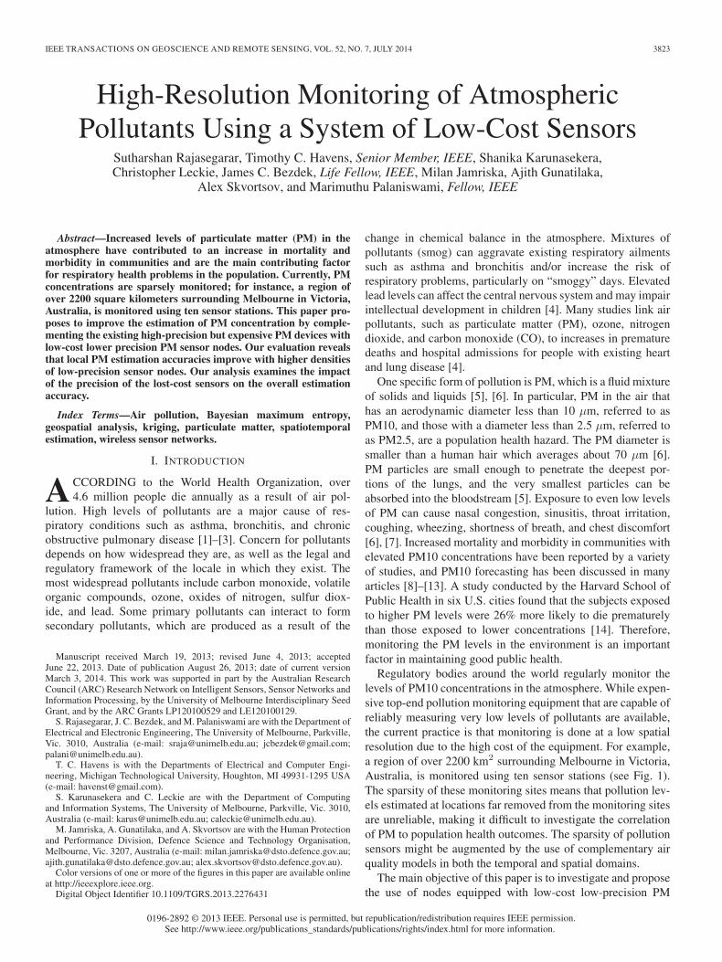
Regulatory bodies around the world regularly monitor thelevels of PM10 concentrations in the atmosphere. While expen-sive top-end pollution monitoring equipment that are capable ofreliably measuring very low levels of pollutants are available,the current practice is that monitoring is done at a low spatialresolution due to the high cost of the equipment. For example,a region of over 2200 km2 surrounding Melbourne in Victoria,Australia, is monitored using ten sensor stations (see Fig. 1).The sparsity of these monitoring sites means that pollution lev-els estimated at locations far removed from the monitoring sitesare unreliable, making it difficult to investigate the correlationof PM to population health outcomes. The sparsity of pollutionsensors might be augmented by the use of complementary airquality models in both the temporal and spatial domains.
The main objective of this paper is to investigate and proposethe use of nodes equipped with low-cost low-precision PM
3824 IEEE TRANSACTIONS ON GEOSCIENCE AND REMOTE SENSING, VOL. 52, NO. 7, JULY 2014
Fig. 1. Geographical locations for the EPAV sensors. The horizontal(east–west) size of the domain is about 55 km, and the vertical (north–south)dimension is about 40 km.
sensors to supplement existing high-precision, often expensive,PM devices with the goal of improving the estimation at finerspatial and temporal resolutions. A more capable sensor net-work [15]–[29] will enable us to get a more accurate measure ofthe exposure of individuals to PM10 concentrations and, hence,better understand the impact of PM10 levels on respiratoryillnesses. To achieve this objective, we perform simulationstudies using synthetically generated PM10 concentration datathat match the overall spatiotemporal characteristics of mea-sured PM10 data. In particular, in this paper, we generatedsynthetic PM10 data that resemble the historical spatiotemporalPM10 data collected by the Environment Protection AuthorityVictoria (EPAV). We consider PM10 concentration time seriesfrom eight sensor stations located in the vicinity of Melbourne.Details of this EPAV sensor deployment can be found at theEnvironment Protection Authority (EPA) Web site [30]. To gen-erate PM10 over the EPAV monitored region for this study, wepropose two space–time (ST) covariance-based noise modelingalgorithms: a Fourier transform-based method and a Choleskydecomposition-based method.
Using the generated simulation data, we analyze how theestimation accuracy of PM10 levels at arbitrary locations isaffected by the following: 1) spatial resolution of sensors and2) sensor accuracy. This was done by estimating PM10 levels ata number of arbitrary locations using generated synthetic sensormeasurements from high-precision EPAV sensors and a speci-fied number of low-precision sensors placed at locations on agrid. The effect of the number and the accuracy of the low-costsensors is studied. We used the Bayesian maximum entropy(BME) technique [31], which is a well-accepted technique forthe estimation and prediction of spatiotemporally correlateddata. Our results show the feasibility of using low-cost low-precision sensors for improving the estimation accuracy ofPM10 data.
II. RELATED WORK
Modeling networks of wireless pollutant sensors have re-cently been a topic of intensive research in applications span-ning from environmental and technological monitoring todefense and security systems (see [32] and [33] and referencestherein). It has been demonstrated that such systems can be
described by a mathematical model that has some similaritieswith population biology. By employing this approach, a numberof optimization strategies and operational protocols have beenproposed to meet various operational criteria, including thetradeoff between parameters of an individual sensor and thecoherent performance of the chemical sensor network andthe integrated system (for details, see [32] and [33]). This papercontributes to this line of research by exploring the informationgain that can be provided by the networking effect in a systemof many sensors, each with low individual accuracy.
A wide variety of sensors and models have been used for theestimation and prediction of air quality and concentrations ofspecific pollutants [34]–[36]. Slini et al. [8] used a stochasticautoregressive integrated moving average (ARIMA) model tostudy and make maximum ozone concentration forecasts inAthens, Greece. Diaz-Robles et al. [9] combined an ARIMAmodel with a neural network (NN) to build a hybrid model toforecast PM10 concentrations in Temuco, Chile. Slini et al.[10] described an operational air quality forecasting modulefor PM10 based on classification and regression trees and NNmethods, which is capable of capturing PM10 concentrationtrends. Stadlober et al. [11] used multiple linear regressionmodels that combined the information of the present day withmeteorological forecasts of the next day to forecast daily PM10concentrations for sites located in the three cities: Bolzano,Klagenfurt, and Graz, the three capitals in the provinces ofSouth Tyrol, Carinthia, and Styria. Tsai et al. [12] studiedPM2.5 and PM10 in Bangkok using simple regression andcorrelation analysis for data gathered in a shopping center andat a university. Yu et al. [37] studied the spatiotemporal distri-bution of PM2.5 across the Taipei area from 2005 to 2007 usinga land use regression model. They established a quantitativerelationship between PM2.5/PM10 and land use informationfor predicting the PM2.5 concentration. Epitropou et al. [38]used a fusion strategy to select environmental information fromopen access web resources of various types and data frommonitoring stations in order to provide tailored information tothe users. Forecast models are produced using published airquality information in the form of color-mapped georeferencedimages and data from chemical weather databases.
Multivariate geostatistics offers many alternatives for choos-ing the family of functions F and a best member F ∗ ∈ Fto describe and model the observations. Good introductionsto some of these methods are the texts by Clark [39] andWackernagel [40]. The most popular and perhaps best knownpossibilities are variograms, ordinary, simple, and weightedkriging, principal component analysis, canonical analysis, andcorrespondence analysis. Christakos et al. [31], [41] present amethod for estimating PM10 levels in the state of Californiabased on an integrated ST domain using the BME mappingapproach. Their BME method is a generalized model, in whichkriging becomes one of the special cases. We use this methodto estimate the concentrations at unknown spatiotemporal loca-tions in the EPAV region.
One of the primary challenges in many of these studies(including ours) is that analysis is based on measurements froma few sparsely located pollution monitors. For example, onesuch study in Santiago, Chile, used the average of just five
RAJASEGARAR et al.: MONITORING OF ATMOSPHERIC POLLUTANTS USING A SYSTEM OF LOW-COST SENSORS 3825
monitoring sites to obtain pollution data representing the wholecity [42]. Localized variations of pollutant concentrations maynot be adequately captured by a small number of sparselylocated monitoring sites; therefore, in [42], Santiago is dividedinto five regions, each centered around a pollution monitoringstation. This strategy seemed to improve correlations betweenpollutant levels and observed health effects throughout the city.Our approach is somewhat different. We first validate our modelwith simulated data at the nodes of a regularized rectangulargrid that circumscribes the sensor stations shown in Fig. 1.Then, we use the time series at the EPAV sites as a basis forboth interpolation and extrapolation over the spatial domainof Fig. 1.
The statistical properties of PM (pollutant, aerosol, moisture,and dust) in the atmospheric boundary layer have been investi-gated; the pioneering work of Richardson and Batchelor [43],[44] is well documented. It is recognized that these propertiesand statistics of associated particle time series emerge from thephysics of turbulent mixing and particle dispersion by randomflow [45], [46]. This enables the development of physics-basedframeworks for data analysis and implementation of rigorouscomputer simulations for the concentration time series (see[45], [47], [48], and references therein). In the context of thecurrent study, two specific properties of particle statistics aremost relevant: 1) The concentration time series are strictlypositive (since measured values are simply counts of particles),and 2) they can be comprehensively characterized by the firsttwo statistical moments [46] (since they are driven by theunderlying Gamma distribution). The latter property becomescritical for the application of the BME model; see (7).
III. PROBLEM STATEMENT AND APPROACH
A. Problem Statement
We consider a ST domain where a general point in spaceand time is given by p = (s, t) ∈ S × T , where s = (x, y) isthe geographical location and t is the time. A set of Nh high-precision sensors and Nl low-precision sensors is deployed atknown geographical locations in the region, and measure PM10concentrations over T discrete time points. Hence, a collec-tion of nh = Nh × T high-precision sensor measurements andnl = Nl × T low-precision sensor measurements is collectedat nd = nh + nl ST points. The aim is to estimate the PM10concentrations at an arbitrary set of nk ST points, called theestimation points, based on the measured values from nd STpoints. Note that nk = Nk × T , where Nk is the number ofgeographic (estimation) locations.
We denote the ST random field realizations (PM10 con-centrations) over the ST region as a collection of correlatedrandom variables Zmap = {Zdata ∪ Zest} at points pmap ={pdata ∪ pest}, where Zdata = (Z1,Z2, . . . ,Znd
), Zest =(Znd+1, . . . ,Znd+k, . . . ,Znk
), pdata = (p1, p2, . . . , pnd), and
pest = (pnd+1, . . . , pnd+k, . . . , pnk).
We define the root-mean-square estimation error εs at aspatial location s over a time period T as
εs =
√√√√ 1
T
T∑ι=1
(Z(s, tι)− Z(s, tι))2 (1)
where Z(s, tι) is the true value of the PM concentration at anST point (s, tι) and Z(s, tι) is the estimated value of the PMconcentration.
The overall root-mean-square error (over space and time) εfor a given sensor configuration is defined as
ε =
√√√√ 1
NkT
Nk∑i=1
T∑ι=1
(Z(si, tι)− Z(si, tι))2. (2)
Our aim is to study the impact of the number of low-precisionsensors (Nl) and their accuracy on the estimation errors (ε, εs).In particular, we are interested in determining whether supple-menting high-precision sensors with low-precision sensors canreduce the error.
B. Our Approach
To study the impact of low-precision sensors on estima-tion accuracy, we need to compare estimated PM values toactual concentrations (ground-truth data) at chosen locations.While the measurements from high-precision sensors are thebest possible estimates of actual concentrations, due to thespatial sparseness of these measurements, there are not enoughground-truth data available to perform the intended analysis.Therefore, the approach that we have taken is to generatesynthetic ground-truth data that resemble the characteristics ofreal data. In this paper, we use the real PM10 data availablefrom eight sensors (later, we will identify the eight sensorsthat we are using that have significantly less missing data)deployed in the region around Melbourne, Australia, by theEPAV. We describe the techniques that we use for this purposein Section IV.
After generating synthetic ground-truth data, the simulatedconcentration time series corresponding to Nh EPAV sensorstation locations are taken as the measurements from the high-precision sensors. We then apply a sensor model to simulatelow-precision sensor measurements made at Nl additional lo-cations. The sensor model allows us to mimic characteristicssuch as noise, saturation, linearity, and the minimum measure-ment threshold of sensors. Then, we use simulated measure-ments corresponding to both high- and low-precision sensorsto estimate PM10 concentrations at a set of arbitrary knownlocations not coinciding with the existing sensor locations. Weuse the BME technique to estimate the concentrations at chosenlocations. The BME technique is described in Section VI.
IV. SYNTHETIC GROUND-TRUTH DATA GENERATION
We propose two ST covariance-based noise modeling al-gorithms to generate ground-truth data that simulate PM10concentrations over the EPAV monitored region. One is basedon the fast Fourier transform (FFT) model, and the other isbased on the Cholesky factorization model. We now formulatethe two ST covariance-modeled noise schemes.
A. FFT Model
Assume a wide sense stationary (WSS) 2-D covariancemodel B(Δx,Δy) for the spatial region. If we assume that
3826 IEEE TRANSACTIONS ON GEOSCIENCE AND REMOTE SENSING, VOL. 52, NO. 7, JULY 2014
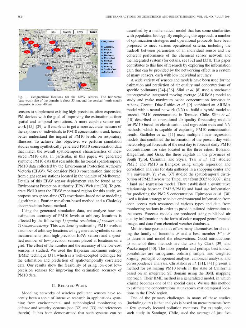
Fig. 2. Example simulated time-series data computed by the FFT model. A Gaussian covariance model was used with parameters υ = 1 and a = 5. (a) t = 1.(b) t = 2. (c) t = 3. (d) t = 4.
B is also isotropic, then it can be written as B(r), where r =‖x− y‖2 is the Euclidean or 2 norm of the vector (x, y). Onesuch model could be the Gaussian B(r) = υe−r2/a2
, where υand a are the parameters of the model.
The most popular way to simulate WSS covariance-modelednoise is by using the FFT. Assume a grid of sensors S ={s11, s12, . . . , sn(m−1), snm}, where sij = (xi, yj) is the sen-sor location. First, we construct the n×m matrix B =[B(rij)]n×m, where rij = ‖sij − sij‖2 and sij is the center ofthe grid. Then, the covariance-modeled noise is constructed asfollows:
1) Compute the 2-D FFT of B, ξB = FFT2D(B).2) Compute the 2-D FFT of an n×m complex Gaussian
white noise matrix W , ξW = FFT2D(W ).3) Compute the 2-D inverse FFT, V =
IFFT2D(√(siB) ◦ (siW )), where ◦ is the Hadamard
product.This produces two noise draws: the real part and the imagi-
nary part of V (here, we use the real part of V ).To add time dependence to this model, we simply construct
an n×m× T matrix B = [rijw]n×m×T , where, now, rijw =‖sijw − sijw‖2 and sijw = (xi, yj , tw). The computation pro-cess is the same as above, except that 3-D FFTs and inverseFFTs are used, and a 3-D complex Gaussian white noiserandom matrix is drawn in step 2.
Fig. 2 shows examples of FFT-simulated time-series dataon a grid. The advantage of the FFT-based model is that itis computationally fast and easy to implement. However, theFFT-based model is limited to a grid arrangement, which maynot be appropriate for simulations of real systems. Hence, wenow move to a different type of model (that produces equivalentresults for arbitrary sensor network locations).
B. Cholesky Factorization Model
Now, consider some collection of sensors S = {s1, . . . , sn},where si = (xi, yi) is the sensor location (not necessarily gridbased). First, we construct an n× n matrix, B = [B(rij)]n×n,where rij = ‖si − sj‖2. B is positive semidefinite and thuscan be factorized into B = RRT (Cholesky factorization).Draw an n-length vector β of unit-variance zero-mean normal-distributed random numbers, and compute φ = Rβ. The co-variance of φ is
Bφ = 〈φφT 〉 = R〈ββT 〉RT = RInRT = B (3)
where 〈·〉 indicates the expected value. Hence, the covarianceof φ is exactly B. The vector φ is a set of simulated sensormeasurements at each location in X according to the statisticalmodel B(r).
Now, assume a time series of sensor measurements S ={S1, . . . , ST }, where St is the tth set of measurements. Con-sider the time-based covariance model Bt(Δt). Construct thematrix Bt = [Bt(Δtij)]T×T , where Δtij = |ti − tj |, factor itas Bt = RtR
Tt , and make a random draw At = RtA, where
A is a T × n matrix of unit-variance zero-mean normally dis-tributed random numbers. Each row of At is an n-length vectorof Bt(0)-variance zero-mean normal-distributed random num-bers. Therefore, 〈(At)
Ti (At)i〉 = Bt(0)In, ∀i, where (At)i
is the ith row of At. Finally, we can create ST covariance-modeled noise by Φ = RAT
t , where Φ = {φ1, . . . ,φT } is thetime series of simulated sensor measurements. Each φt has thespatial statistics of B(r), and the time series at each sensorlocation has the temporal statistics of Bt(Δt). The advantageof this method is that it is not constrained to a grid-based sensorarrangement (as the FFT model is). Fig. 3 illustrates using theCholesky method to simulate the sensor measurements of theEPA Victoria sensor array (ten locations).
V. MODEL FITTING TO REAL EPA DATA
The first step to fitting a WSS spatially isotropic spatiotem-poral covariance model to real data is to compute the variogram(covariance estimate) of the sensor measurements z(s, t). Sincewe are assuming an isotropic WSS model of the form B(r, t) =Bs(r)Bt(Δt), we can model the spatial and temporal covari-ances separately. The basic steps of this process are as follows.
1) Compute the spatial variogram Bs(r) and temporal vari-ogram Bt(Δt) from the data z(s, t).
2) (Optional) Interpolate the variogram(s) onto a uniformgrid.
3) Regress parameterized models to each of Bs(r) andBr(Δt).
4) Choose the best spatial model and the best temporalmodel (if more than one model were regressed to eachvariogram).
In detail, the first step is to calculate the variograms, viz.,covariance estimates. The isotropic spatial covariance estimate
RAJASEGARAR et al.: MONITORING OF ATMOSPHERIC POLLUTANTS USING A SYSTEM OF LOW-COST SENSORS 3827
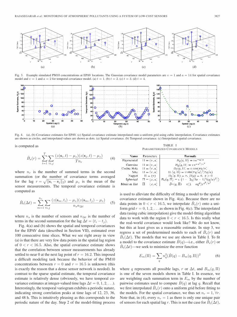
Fig. 3. Example simulated PM10 concentrations at EPAV locations. The Gaussian covariance model parameters are υ = 1 and a = 14 for spatial covariancemodel and υ = 1 and a = 2 for temporal covariance model. (a) t = 1. (b) t = 2. (c) t = 3. (d) t = 4.
Fig. 4. (a), (b) Covariance estimates for EPAV. (c) Spatial covariance estimate interpolated onto a uniform grid using cubic interpolation. Covariance estimatesare shown as circles, and interpolated values are shown as dots. (a) Spatial covariance. (b) Temporal covariance. (c) Interpolated spatial covariance.
is computed as
Bs(r) =
T∑t=1
∑∀i,j
(z(si, t)− μz)(z(sj , t)− μz)
Tnr(4)
where nr is the number of summed terms in the secondsummation (or the number of covariance terms averagedfor the lag r =
√‖si − sj‖2) and μz is the mean of the
sensor measurements. The temporal covariance estimate iscomputed as
Bt(Δt) =
ns∑m=1
∑∀i,j
(z(sm, ti)− μz)(z(sm, tj)− μz)
nsnΔt(5)
where ns is the number of sensors and nΔt is the number ofterms in the second summation for the lag Δt = (ti − tj).
Fig. 4(a) and (b) shows the spatial and temporal covariancesfor the EPAV data (described in Section VII), estimated over100 consecutive time slices. What we see right away in view(a) is that there are very few data points in the spatial lag regionof 0 < r < 16.5. Also, the spatial covariance estimate showsthat the correlation between sensor measurements has alreadysettled to near 0 at the next lag point of r = 16.2. This imposeda difficult modeling task because the behavior of the PM10concentrations between r = 0 and r = 16.5 is unknown (thisis exactly the reason that a dense sensor network is needed). Incontrast to the sparse spatial estimate, the temporal covarianceestimate is relatively dense (obviously, we have temporal co-variance estimates at integer-valued time lags Δt = 0, 1, 2, . . .).Interestingly, the temporal variogram exhibits a periodic nature,indicating strong correlation peaks at time lags of 12, 23, 36,and 48 h. This is intuitively pleasing as this corresponds to theperiodic nature of the day. Step 2 of the model-fitting process
TABLE IPARAMETERIZED COVARIANCE MODELS
is used to alleviate the difficulty of fitting a model to the spatialcovariance estimate shown in Fig. 4(a). Because there are nodata points in 0 < r < 16.5, we interpolate Bs(r) onto a uni-form grid r = 0, 1, 2, . . . as shown in Fig. 4(c). The interpolateddata (using cubic interpolation) give the model-fitting algorithmdata to work with the region 0 < r < 16.5. Is this really whatthe real-world covariance would look like? We do not know,but this at least gives us a reasonable estimate. In step 3, weregress a set of predetermined models to each of Bs(r) andBt(Δt). The models that we use are shown in Table I. To fita model to the covariance estimate B(q)—i.e., either Bs(r) orBt(Δt)—we seek to minimize the error function
Em(Π) =∑q
n2q(B(q)−Bm(q,Π))2 (6)
where q represents all possible lags, r or Δt, and Bm(q,Π)is one of the seven models shown in Table I. In essence, weare weighting each summation term in Em by the number ofpairwise estimates used to compute B(q) at lag q. Recall thatwe first interpolated Bs(r) onto a uniform grid before fitting tothe models. For the spatial covariance, we thus set nr = 1, ∀r.Note that, in (4), every nr = 1 as there is only one unique pairof sensors for each spatial lag r. This is not the case for Bt(Δt),
3828 IEEE TRANSACTIONS ON GEOSCIENCE AND REMOTE SENSING, VOL. 52, NO. 7, JULY 2014
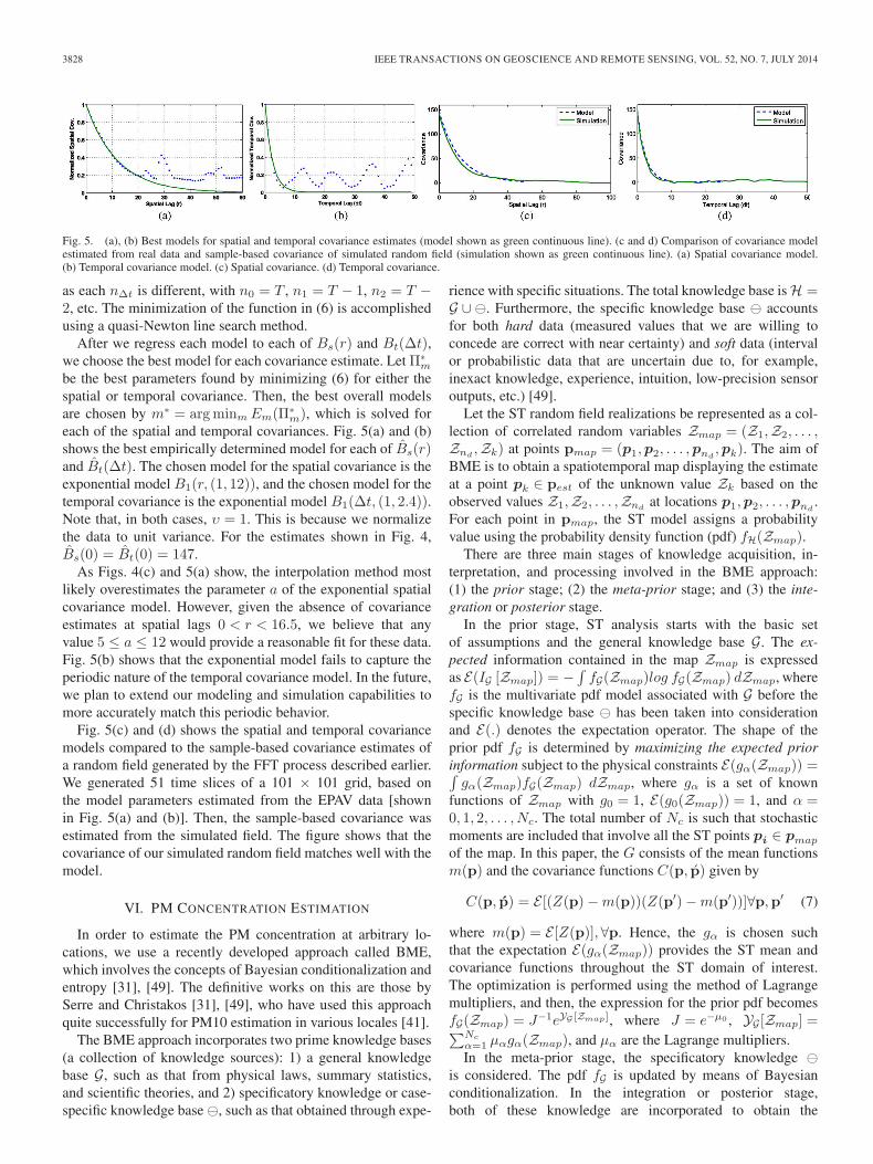
Fig. 5. (a), (b) Best models for spatial and temporal covariance estimates (model shown as green continuous line). (c and d) Comparison of covariance modelestimated from real data and sample-based covariance of simulated random field (simulation shown as green continuous line). (a) Spatial covariance model.(b) Temporal covariance model. (c) Spatial covariance. (d) Temporal covariance.
as each nΔt is different, with n0 = T , n1 = T − 1, n2 = T −2, etc. The minimization of the function in (6) is accomplishedusing a quasi-Newton line search method.
After we regress each model to each of Bs(r) and Bt(Δt),we choose the best model for each covariance estimate. Let Π∗
m
be the best parameters found by minimizing (6) for either thespatial or temporal covariance. Then, the best overall modelsare chosen by m∗ = argminm Em(Π∗
m), which is solved foreach of the spatial and temporal covariances. Fig. 5(a) and (b)shows the best empirically determined model for each of Bs(r)and Bt(Δt). The chosen model for the spatial covariance is theexponential model B1(r, (1, 12)), and the chosen model for thetemporal covariance is the exponential model B1(Δt, (1, 2.4)).Note that, in both cases, υ = 1. This is because we normalizethe data to unit variance. For the estimates shown in Fig. 4,Bs(0) = Bt(0) = 147.
As Figs. 4(c) and 5(a) show, the interpolation method mostlikely overestimates the parameter a of the exponential spatialcovariance model. However, given the absence of covarianceestimates at spatial lags 0 < r < 16.5, we believe that anyvalue 5 ≤ a ≤ 12 would provide a reasonable fit for these data.Fig. 5(b) shows that the exponential model fails to capture theperiodic nature of the temporal covariance model. In the future,we plan to extend our modeling and simulation capabilities tomore accurately match this periodic behavior.
Fig. 5(c) and (d) shows the spatial and temporal covariancemodels compared to the sample-based covariance estimates ofa random field generated by the FFT process described earlier.We generated 51 time slices of a 101 × 101 grid, based onthe model parameters estimated from the EPAV data [shownin Fig. 5(a) and (b)]. Then, the sample-based covariance wasestimated from the simulated field. The figure shows that thecovariance of our simulated random field matches well with themodel.
VI. PM CONCENTRATION ESTIMATION
In order to estimate the PM concentration at arbitrary lo-cations, we use a recently developed approach called BME,which involves the concepts of Bayesian conditionalization andentropy [31], [49]. The definitive works on this are those bySerre and Christakos [31], [49], who have used this approachquite successfully for PM10 estimation in various locales [41].
The BME approach incorporates two prime knowledge bases(a collection of knowledge sources): 1) a general knowledgebase G, such as that from physical laws, summary statistics,and scientific theories, and 2) specificatory knowledge or case-specific knowledge base �, such as that obtained through expe-
rience with specific situations. The total knowledge base is H =G ∪ �. Furthermore, the specific knowledge base � accountsfor both hard data (measured values that we are willing toconcede are correct with near certainty) and soft data (intervalor probabilistic data that are uncertain due to, for example,inexact knowledge, experience, intuition, low-precision sensoroutputs, etc.) [49].
Let the ST random field realizations be represented as a col-lection of correlated random variables Zmap = (Z1,Z2, . . . ,Znd
,Zk) at points pmap = (p1,p2, . . . ,pnd,pk). The aim of
BME is to obtain a spatiotemporal map displaying the estimateat a point pk ∈ pest of the unknown value Zk based on theobserved values Z1,Z2, . . . ,Znd
at locations p1,p2, . . . ,pnd.
For each point in pmap, the ST model assigns a probabilityvalue using the probability density function (pdf) fH(Zmap).
There are three main stages of knowledge acquisition, in-terpretation, and processing involved in the BME approach:(1) the prior stage; (2) the meta-prior stage; and (3) the inte-gration or posterior stage.
In the prior stage, ST analysis starts with the basic setof assumptions and the general knowledge base G. The ex-pected information contained in the map Zmap is expressedas E(IG [Zmap]) = −
∫fG(Zmap)log fG(Zmap) dZmap, where
fG is the multivariate pdf model associated with G before thespecific knowledge base � has been taken into considerationand E(.) denotes the expectation operator. The shape of theprior pdf fG is determined by maximizing the expected priorinformation subject to the physical constraints E(gα(Zmap)) =∫gα(Zmap)fG(Zmap) dZmap, where gα is a set of known
functions of Zmap with g0 = 1, E(g0(Zmap)) = 1, and α =0, 1, 2, . . . , Nc. The total number of Nc is such that stochasticmoments are included that involve all the ST points pi ∈ pmap
of the map. In this paper, the G consists of the mean functionsm(p) and the covariance functions C(p, p) given by
C(p, p) = E [(Z(p)−m(p))(Z(p′)−m(p′))]∀p,p′ (7)
where m(p) = E [Z(p)], ∀p. Hence, the gα is chosen suchthat the expectation E(gα(Zmap)) provides the ST mean andcovariance functions throughout the ST domain of interest.The optimization is performed using the method of Lagrangemultipliers, and then, the expression for the prior pdf becomesfG(Zmap) = J−1eYG [Zmap], where J = e−μ0 , YG [Zmap] =∑Nc
α=1 μαgα(Zmap), and μα are the Lagrange multipliers.In the meta-prior stage, the specificatory knowledge �
is considered. The pdf fG is updated by means of Bayesianconditionalization. In the integration or posterior stage,both of these knowledge are incorporated to obtain the
RAJASEGARAR et al.: MONITORING OF ATMOSPHERIC POLLUTANTS USING A SYSTEM OF LOW-COST SENSORS 3829
posterior pdf fH(Zmap) = Q−1Y�[YG ,�,Zmap], where Q isa normalization parameter. If we assume that the specificknowledge � consists of the hard data and the probabilisticsoft data, then the posterior operator Y� becomes Y� =Q−1
∫I e
YG [Zmap]dF�[Zsoft], where � : Zsoft ∈ I,Prob�[zsoft ≤ ζ]=F�(ζ) and Q=
∫I dF�(Zsoft)fG(Zdata).
Zsoft denotes the soft data, I denotes the domain of Zsoft,Zhard denotes the hard data, Zdata = {Zhard ∪ Zsoft} ⊂Zmap, and F� is the cumulative distribution function obtainedfrom �. Several possibilities exist to obtain the estimate Zk atan unknown point pk using fH(Zmap). One such possibilityis to use the mean estimate at the point pk, which is given byZk,mean =
∫ZkfH(Zk)dZk. In this paper, this mean estimate
is used to find the PM10 concentrations at the off-sensorlocations. Note that this BME mean estimate minimizes themean squared estimation error.
Let the ST variability of the PM10 concentration Z be de-scribed in terms of a (centered) covariance function C(κ, τ) =E [(Z(p)−m(p))((Z(p′)−m(p′))], where p− p′ = ((s−s′), (t− t′));κ = ‖s− s′‖; τ = |t− t′| and m is the mean. Thequantities κ and τ are space and time lags and show that thiscovariance is spatially isotropic and stationary in time. For thecase of κ = 0, C(0, τ) is reduced to the single-point time series(observations from an individual sensor) and can easily bevalidated experimentally [45]. More specifically, the differenceC(κ, τ)− C(0, 0) should exhibit a linear dependence on itsarguments at the limit of small values of κ, τ [46]. Since thisproperty has been reliably recovered experimentally [45], it canbe used as a supporting argument for the proposed model.
We use C(κ, τ) = υsυte(−κ/as)e(−τ/at) to model the covari-
ance structure in the evaluation. The covariance coefficients υsand υt provide information about variations in the PM10 distri-bution. The coefficient as is the range of spatial variation, andat represents temporal fluctuations. We match the coefficientsto our generated simulation data, which are a representation ofthe EPAV PM10 data (as explained in Section V), and utilizethe BME software for the estimation [50].
VII. EVALUATION
A. Representation of the EPAV Sensor Network
Our work is facilitated by introducing the artificial Cartesiancoordinate system for the EPAV nodes (shown in Fig. 1) ona regular grid of size 200 × 200. The EPAV nodes consid-ered in this evaluation are deployed at the following eightlocations (including the coordinates): Alphington (141, 171),Box Hill (159, 156), Brighton (135, 122), Dandenong (177,89), Mooroolbark (197, 170), Deer Park (89, 176), Footscray(115, 164), and Richmond (135, 156). The EPAV PM10 data(high-precision sensor data) were collected during the periodbetween October 3, 2011 and April 20, 2012 at a samplinginterval of 1 h. We use the FFT-based model (grid sensor-basedscheme; see Section IV-A) for generating the ground-truth datafor our experiments as the given sensor locations are already ona Cartesian grid.
The ground-truth data are generated for a 3-D rectangu-lar parallelepiped (rectangular box) region spanned by the
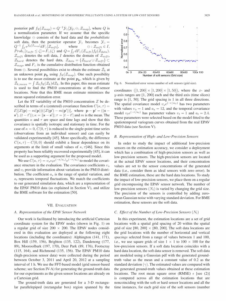
Fig. 6. Normalized error versus number of soft sensors (grid size).
coordinates ([1, 200]× [1, 200]× [1, 50]), where the x- andy-axis ranges are [1, 200] each and the third axis (time slices)range is [1, 50]. The grid spacing is 1 in all three directions.The spatial covariance model υse(−r/aS) has two parameterswith values υs = 1 and as = 12, and the temporal covariancemodel υte(−r/at) has parameter values υt = 1 and at = 2.4.These parameters were selected based on the model fitted to thespatiotemporal variogram curves obtained from the real EPAVPM10 data (see Section V).
B. Representation of High- and Low-Precision Sensors
In order to study the impact of additional low-precisionsensors on the estimation accuracy, we consider a deploymentwhich has a combination of high-precision sensors as well aslow-precision sensors. The high-precision sensors are locatedat the actual EPAV sensor locations, and their concentrationvalues are set to the sensor concentrations of the generateddata (i.e., consider them as ideal sensors with zero error). Inthe BME estimation, these are the hard data locations. To studythe impact of low-precision sensors, we place them on a regulargrid encompassing the EPAV sensor network. The number oflow-precision sensors (Nl) is varied by changing the grid size.The precision of the sensors is controlled by adding zero-mean Gaussian noise with varying standard deviation. For BMEestimation, these sensors are the soft data.
C. Effect of the Number of Low-Precision Sensors (Nl)
In this experiment, the estimation locations are a set of gridlocations with a spatial grid spacing of 20 within the spatialgrid of size [80, 200] × [80, 200]. The soft data locations arethe grid locations with the number of horizontal and verticalspacings selected from a range of values between 1 and 100,i.e., we use square grids of size 1 × 1 to 100 × 100 for thelow-precision sensors. If a soft data location coincides with ahard data location, the soft data sensor is removed. The soft dataare modeled using a Gaussian pdf with the generated ground-truth value as the mean and a constant value of 0.2 as thestandard deviation (γ). The estimated values are compared withthe generated ground-truth values obtained at these estimationlocations. The root mean square error (RMSE) ε [see (2)]is computed across all the estimation locations that arenoncoinciding with the soft or hard sensor locations and all thetime instances, for each grid size of the soft sensors (number
3830 IEEE TRANSACTIONS ON GEOSCIENCE AND REMOTE SENSING, VOL. 52, NO. 7, JULY 2014
of soft data locations). The normalized error for each grid sizeof the soft sensors is computed by dividing the RMSE ε bythe RMSE obtained for the hard only case, where there are nolow-precision sensors deployed, i.e., Nl = 0. Fig. 6 shows thenormalized error versus the number of soft sensors. As intuitionwould suggest, the normalized error decreases as the number ofsoft sensors is increased.
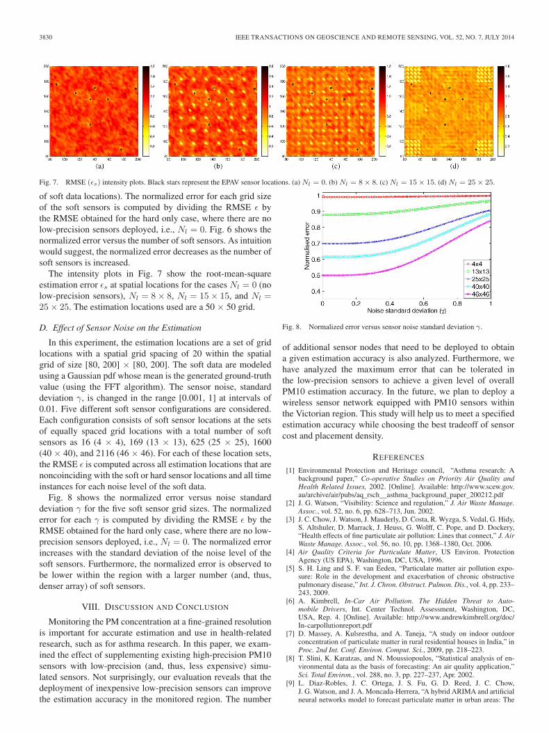
The intensity plots in Fig. 7 show the root-mean-squareestimation error εs at spatial locations for the cases Nl = 0 (nolow-precision sensors), Nl = 8× 8, Nl = 15× 15, and Nl =25× 25. The estimation locations used are a 50 × 50 grid.
D. Effect of Sensor Noise on the Estimation
In this experiment, the estimation locations are a set of gridlocations with a spatial grid spacing of 20 within the spatialgrid of size [80, 200] × [80, 200]. The soft data are modeledusing a Gaussian pdf whose mean is the generated ground-truthvalue (using the FFT algorithm). The sensor noise, standarddeviation γ, is changed in the range [0.001, 1] at intervals of0.01. Five different soft sensor configurations are considered.Each configuration consists of soft sensor locations at the setsof equally spaced grid locations with a total number of softsensors as 16 (4 × 4), 169 (13 × 13), 625 (25 × 25), 1600(40 × 40), and 2116 (46 × 46). For each of these location sets,the RMSE ε is computed across all estimation locations that arenoncoinciding with the soft or hard sensor locations and all timeinstances for each noise level of the soft data.
Fig. 8 shows the normalized error versus noise standarddeviation γ for the five soft sensor grid sizes. The normalizederror for each γ is computed by dividing the RMSE ε by theRMSE obtained for the hard only case, where there are no low-precision sensors deployed, i.e., Nl = 0. The normalized errorincreases with the standard deviation of the noise level of thesoft sensors. Furthermore, the normalized error is observed tobe lower within the region with a larger number (and, thus,denser array) of soft sensors.
VIII. DISCUSSION AND CONCLUSION
Monitoring the PM concentration at a fine-grained resolutionis important for accurate estimation and use in health-relatedresearch, such as for asthma research. In this paper, we exam-ined the effect of supplementing existing high-precision PM10sensors with low-precision (and, thus, less expensive) simu-lated sensors. Not surprisingly, our evaluation reveals that thedeployment of inexpensive low-precision sensors can improvethe estimation accuracy in the monitored region. The number
Fig. 8. Normalized error versus sensor noise standard deviation γ.
of additional sensor nodes that need to be deployed to obtaina given estimation accuracy is also analyzed. Furthermore, wehave analyzed the maximum error that can be tolerated inthe low-precision sensors to achieve a given level of overallPM10 estimation accuracy. In the future, we plan to deploy awireless sensor network equipped with PM10 sensors withinthe Victorian region. This study will help us to meet a specifiedestimation accuracy while choosing the best tradeoff of sensorcost and placement density.
REFERENCES
[1] Environmental Protection and Heritage council, “Asthma research: Abackground paper,” Co-operative Studies on Priority Air Quality andHealth Related Issues, 2002. [Online]. Available: http://www.scew.gov.au/archive/air/pubs/aq_rsch__asthma_background_paper_200212.pdf
[2] J. G. Watson, “Visibility: Science and regulation,” J. Air Waste Manage.Assoc., vol. 52, no. 6, pp. 628–713, Jun. 2002.
[3] J. C. Chow, J. Watson, J. Mauderly, D. Costa, R. Wyzga, S. Vedal, G. Hidy,S. Altshuler, D. Marrack, J. Heuss, G. Wolff, C. Pope, and D. Dockery,“Health effects of fine particulate air pollution: Lines that connect,” J. AirWaste Manage. Assoc., vol. 56, no. 10, pp. 1368–1380, Oct. 2006.
[4] Air Quality Criteria for Particulate Matter, US Environ. ProtectionAgency (US EPA), Washington, DC, USA, 1996.
[5] S. H. Ling and S. F. van Eeden, “Particulate matter air pollution expo-sure: Role in the development and exacerbation of chronic obstructivepulmonary disease,” Int. J. Chron. Obstruct. Pulmon. Dis., vol. 4, pp. 233–243, 2009.
[6] A. Kimbrell, In-Car Air Pollution. The Hidden Threat to Auto-mobile Drivers, Int. Center Technol. Assessment, Washington, DC,USA, Rep. 4. [Online]. Available: http://www.andrewkimbrell.org/doc/In-carpollutionreport.pdf
[7] D. Massey, A. Kulsrestha, and A. Taneja, “A study on indoor outdoorconcentration of particulate matter in rural residential houses in India,” inProc. 2nd Int. Conf. Environ. Comput. Sci., 2009, pp. 218–223.
[8] T. Slini, K. Karatzas, and N. Moussiopoulos, “Statistical analysis of en-vironmental data as the basis of forecasting: An air quality application,”Sci. Total Environ., vol. 288, no. 3, pp. 227–237, Apr. 2002.
[9] L. Diaz-Robles, J. C. Ortega, J. S. Fu, G. D. Reed, J. C. Chow,J. G. Watson, and J. A. Moncada-Herrera, “A hybrid ARIMA and artificialneural networks model to forecast particulate matter in urban areas: The
RAJASEGARAR et al.: MONITORING OF ATMOSPHERIC POLLUTANTS USING A SYSTEM OF LOW-COST SENSORS 3831
case of Temuco, Chile,” Atmos. Environ., vol. 42, no. 35, pp. 8331–8340,Nov. 2008.
[10] T. Slini, A. Kaprara, K. Karatzas, and N. Moussiopoulos, “ PM10 fore-casting for Thessaloniki, Greece,” Environ. Modell. Softw., vol. 21, no. 4,pp. 559–565, Apr. 2006.
[11] E. Stadlober, S. Hormann, and B. Pfeiler, “Quality and performance of aPM10 daily forecasting model,” Atmos. Environ., vol. 42, no. 6, pp. 1098–1109, Feb. 2008.
[12] F. C. Tsai, K. R. Smith, N. Vichit-Vadakan, B. D. Ostro, L. G. Chestnut,and N. Kungskulniti, “Indoor/outdoor PM10 and PM2.5 in Bankok, Thai-land,” J. Exposure Anal. Environ. Epidemiol., vol. 10, no. 1, pp. 15–26,Jan./Feb. 2000.
[13] L. Guoxing, S. Jing, J. S. Rohan, P. X. Chuan, Z. Maigeng, W. Xuying,C. Yue, S. Ross, and S. G. Reginald, “Temperature modifies the effectsof particulate matter on non-accidental mortality: A comparative study ofBeijing, China and Brisbane, Australia,” Public Health Res., vol. 2, no. 2,pp. 21–27, 2012.
[14] D. W. Dockery, C. A. Pope, X. Xu, J. D. Spengler, J. H. Ware,M. E. Fay, J. Benjamin, G. Ferris, and F. E. Speizer, “An associationbetween air pollution and mortality in six cities,” New Engl. J. Med.,vol. 329, no. 24, pp. 1753–1759, Dec. 1993.
[15] S. Rajasegarar, C. Leckie, and M. Palaniswami, “Detecting data anoma-lies in sensor networks,” in Security in Ad-hoc and Sensor Networks,R. Beyah, J. McNair, and C. Corbett, Eds. Singapore: World Scientific,Jul. 2009, pp. 231–260.
[16] J. C. Bezdek, S. Rajasegarar, M. Moshtaghi, C. Leckie, M. Palaniswami,and T. Havens, “Anomaly detection in environmental monitoring net-works,” IEEE Comput. Intell. Mag., vol. 6, no. 2, pp. 52–58, May 2011.
[17] S. Rajasegarar, C. Leckie, and M. Palaniswami, “Anomaly detectionin wireless sensor networks,” IEEE Wireless Commun., vol. 15, no. 4,pp. 34–40, Aug. 2008.
[18] S. Rajasegarar, C. Leckie, M. Palaniswami, and J. C. Bezdek, “Distributedanomaly detection in wireless sensor networks,” in Proc. ICCS, 2006,pp. 1–5.
[19] S. Rajasegarar, J. C. Bezdek, C. Leckie, and M. Palaniswami, “Ellipticalanomalies in wireless sensor networks,” ACM Trans. Sens. Netw., vol. 6,no. 1, p. 28, Dec. 2009.
[20] M. Takruri, S. Rajasegarar, S. Challa, C. Leckie, and M. Palaniswami,“Spatio-temporal modelling based drift aware wireless sensor networks,”IET Wireless Sens. Syst., vol. 1, no. 2, pp. 110–122, Jun. 2011.
[21] S. Rajasegarar, C. Leckie, J. C. Bezdek, and M. Palaniswami, “Centeredhyperspherical and hyperellipsoidal one-class support vector machinesfor anomaly detection in sensor networks,” IEEE Trans. Inf. ForensicsSecurity, vol. 5, no. 3, pp. 518–533, Sep. 2010.
[22] A. Shilton, S. Rajasegarar, and M. Palaniswami, “Combined multiclassclassification and anomaly detection for large-scale wireless sensor net-works,” in Proc. IEEE 8th Int. Conf. Intell. Sens., Sens. Netw. Inf. Process.,Melbourne, VIC, Austrlia, Apr. 2013, pp. 491–496.
[23] M. Moshtaghi, S. Rajasegarar, C. Leckie, and S. Karunasekera, “An effi-cient hyperellipsoidal clustering algorithm for resource-constrained envi-ronments,” Pattern Recognit., vol. 44, no. 9, pp. 2197–2209, Sep. 2011.
[24] M. Moshtaghi, T. Havens, L. Park, J. C. Bezdek, S. Rajasegarar,C. Leckie, M. Palaniswami, and J. Keller, “Clustering ellipses for anomalydetection,” Pattern Recognit., vol. 44, no. 1, pp. 55–69, Jan. 2011.
[25] S. Rajasegarar, A. Shilton, C. Leckie, R. Kotagiri, and M. Palaniswami,“Distributed training of multiclass conic-segmentation support vectormachines on communication constrained networks,” in Proc. 6th Int.Conf. Intell. Sens., Sens. Netw. Inf. Process., Brisbane, QLD, Austrlia,Dec. 2010, pp. 211–216.
[26] M. Moshtaghi, J. C. Bezdek, T. C. Havens, C. Leckie, S. Karunasekera,S. Rajasegarar, and M. Palaniswami, “Streaming analysis in wirelesssensor networks,” Wireless Commun. Mobile Comput., 2012. [Online].Available: http://onlinelibrary.wiley.com/doi/10.1002/wcm.2248/pdf
[27] C. Oreilly, A. Gluhak, M. A. Imran, and S. Rajasegarar, “Online anomalyrate parameter tracking for anomaly detection in wireless sensor net-works,” in Proc. IEEE Conf. Sens., Mesh Ad Hoc Commun. Netw., Seoul,Korea, Jun. 2012, pp. 191–199.
[28] J. Gubbi, R. Buyya, S. Marusic, and M. Palaniswami, “Internet of things(IoT): A vision, architectural elements, and future directions,” FutureGener. Comput. Syst., vol. 29, no. 7, pp. 1645–1660, Sep. 2013.
[29] Internet of Things, 2013. [Online]. Available: http://issnip.unimelb.edu.au/research_program/Internet_of_Things
[32] C. Mendis, A. Skvortsov, A. Gunatilaka, and S. Karunasekera, “Perfor-mance of wireless chemical sensor network with dynamic collaboration,”IEEE Sensors J., vol. 12, no. 8, pp. 2630–2637, Aug. 2012.
[33] S. Karunasekera, C. Mendis, A. Skvortsov, and A. Gunatilaka, “A de-centralized dynamic sensor activation protocol for chemical sensor net-works,” in Proc. 9th IEEE NCA, Jul. 15–17, 2010, pp. 218–223.
[34] H.-h. K. Burke, “Detection of regional air pollution episodes utilizingsatellite digital data in the visual range,” IEEE Trans. Geosci. RemoteSens., vol. GE-20, no. 2, pp. 154–158, Apr. 1982.
[35] F. Cuccoli, L. Facheris, S. Tanelli, and D. Giuli, “Infrared tomographicsystem for monitoring the two-dimensional distribution of atmosphericpollution over limited areas,” IEEE Trans. Geosci. Remote Sens., vol. 38,no. 1, pp. 155–168, Jan. 2000.
[36] A. Srivastava, N. Oza, and J. Stroeve, “Virtual sensors: Using data miningtechniques to efficiently estimate remote sensing spectra,” IEEE Trans.Geosci. Remote Sens., vol. 43, no. 3, pp. 590–600, Mar. 2005.
[37] H.-L. Yu, C.-H. Wang, M.-C. Liu, and Y.-M. Kuo, “Estimation of fineparticulate matter in Taipei using land use regression and Bayesian maxi-mum entropy methods,” Int. J. Environ. Res. Public Health, vol. 8, no. 6,pp. 2153–2169, Jun. 2011.
[38] V. Epitropou, L. Johansson, K. D. Karatzas1, A. Bassoukos,A. Karppinen, J. Kukkonen, and M. Haakana, “Fusion of environmentalinformation for the delivery of orchestrated services for the atmosphericenvironment in the pescado project,” in Proc. Int. Congr. Environ. Modell.Softw. Manag. Resources Limited Planet, R. Seppelt, A. A. Voinovr,S. Lange, and D. Bankamp, Eds., 2012. [Online]. Available: http://www.iemss.org/society/index.php/iemss-2012-proceedings
[40] H. Wackernagle, Multivariate Geostatistics: An Introduction WithApplications. Berlin, Germany: Springer-Verlag, 1998.
[41] G. Christakos, M. L. Serre, and J. Kovitz, “BME representation of partic-ulate matter distributions in the state of California on the basis of uncer-tain measurements,” J. Geophys. Res., vol. 106, no. D9, pp. 9717–9731,May 2001.
[42] B. Ostro, J. M. Sanchez, C. Aranda, and G. S. Eskeland, “Air pollution andmortality,” in Policy Research Working Paper 1453. Washington, DC,USA: The World Bank, 1995, pp. 1–40.
[43] G. K. Batchelor, “Diffusion in a field of homogeneous turbulenceii. Therelative motion of particles,” Math. Proc. Cambridge Philosop. Soc.,vol. 48, no. 2, pp. 345–362, Apr. 1952.
[44] L. F. Richardson, “Atmospheric diffusion shown on a distance-neighbourgraph,” Proc. R. Soc. Lond. A, vol. 110, no. 756, pp. 709–737, Apr. 1926.
[45] M. Jamriska, T. DuBois, and A. Skvortsov, “Statistical characterisationof bio-aerosol background in an urban environment,” Atmos. Environ.,vol. 54, pp. 439–448, Jul. 2012.
[46] E. Yee and A. Skvortsov, “Scalar fluctuations from a point source in aturbulent boundary layer,” Phys. Rev. E, vol. 84, no. 3, pp. 036306-1–036306-7, Sep. 2011.
[47] A. Gunatilaka and R. Gailis, “High fidelity simulation of hazardousplume concentration time series based on models of turbulent disper-sion,” in Proc. 15th Int. Conf. Inf. FUSION, Singapore, Jul. 9–12, 2012,pp. 1838–1845.
[48] G. Boffetta, A. Celani, A. Crisanti, and A. Vulpiani, “Pair dispersionin synthetic fully developed turbulence,” Phys. Rev. E, vol. 60, no. 6,pp. 6734–6741, Dec. 1999.
[49] G. Christakos, Modern Spatiotemporal Geostatistics. New York, NY,USA: Dover, 2012.
Sutharshan Rajasegarar received the B.Sc. Engi-neering degree (with first class honors) in electronicand telecommunication engineering from the Univer-sity of Moratuwa, Moratuwa, Sri Lanka, in 2002 andthe Ph.D. degree from The University of Melbourne,Parkville, Australia, in 2009.
He is currently a Research Fellow with the De-partment of Electrical and Electronic Engineering,The University of Melbourne. His research interestsinclude wireless sensor networks, anomaly/outlierdetection, spatiotemporal estimations, Internet of
things, machine learning, pattern recognition, signal processing, and wirelesscommunication.
3832 IEEE TRANSACTIONS ON GEOSCIENCE AND REMOTE SENSING, VOL. 52, NO. 7, JULY 2014
Timothy C. Havens (S’06–M’106–SM’10) receivedthe Ph.D. degree in electrical and computer engineer-ing from the University of Missouri, Columbia, MO,USA, in 2000.
He is an Assistant Professor in the Departments ofElectrical and Computer Engineering and ComputerScience and the William and Gloria Jackson As-sistant Professor of Computer Systems at MichiganTechnological University, Houghton, MI, USA. Priorto his current position, he was an National ScienceFoundation/Computing Research Association Com-
puting Innovation Fellow at Michigan State University, Lansing, MI, USA.Before working on his Ph.D., he was an Associate Technical Staff at the Mas-sachusetts Institute of Technology, Lincoln Laboratory. His research interestsinclude mobile robotics, explosive hazard detection, heterogeneous and bigdata, social networks, fuzzy sets, sensor networks, and data fusion. He hascoauthored over 50 technical publications.
Dr. Havens was the recipient of the Best Overall Paper Award at IEEEInternational Conference on Fuzzy Systems 2013, the IEEE Franklin V. TaylorAward, and a Best Paper Award from the Midwest Nursing Research Society.He is an Associate Editor of the IEEE TRANSACTIONS ON FUZZY SYSTEMS.
Shanika Karunasekera received the B.Sc degreein electronics and telecommunications engineeringfrom the University of Moratuwa, Moratuwa, SriLanka, in 1990 and the Ph.D. degree in electri-cal engineering from the University of Cambridge,Cambridge, U.K., in 1995.
From 1995 to 2002, she was a Software Engineerand a Distinguished Member of the Technical Staff atLucent Technologies, Bell Labs Innovations, MurrayHill, NJ, USA. In January 2003, she joined theDepartment of Computing and Information Systems,
The University of Melbourne, Parkville, Australia, where she is currentlyan Associate Professor. Her current research interests include decentralizedalgorithms for event and anomaly detection, and decentralized data aggregation.
Christopher Leckie received the B.Sc. degree, theB.E. degree (with first class honors) in electricaland computer systems engineering, and the Ph.D.degree in computer science from Monash Univer-sity, Melbourne, Australia, in 1985, 1987, and 1992,respectively.
He joined Telstra Research Laboratories in 1988,where he conducted research and development intoartificial intelligence techniques for various telecom-munication applications. In 2000, he joined TheUniversity of Melbourne, Parkville, Australia, where
he is currently a Professor in the Department of Computing and InformationSystems. His research interests include scalable data mining, network intrusiondetection, bioinformatics, and wireless sensor networks.
James C. Bezdek (M’80–SM’90–F’92–LF’10) re-ceived the Ph.D. degree in applied mathematics fromCornell University, Ithaca, NY, USA, in 1973.
His interests include optimization, pattern recog-nition, clustering in very large data, coclustering, andvisual clustering. He retired in 2007.
Dr. Bezdek is the past President of the NorthAmerican Fuzzy Information Processing Society, theInternational Fuzzy Systems Association (IFSA),and the IEEE Computational Intelligence Society(CIS), the founding Editor of the International Jour-
nal Approximate Reasoning and the IEEE TRANSACTIONS ON FUZZY SYS-TEMS, a Life Fellow of the and IFSA, and a recipient of the IEEE 3rdMillennium, IEEE CIS Fuzzy Systems Pioneer, IEEE technical field awardRosenblatt, and the Kampe de Feriet medals.
Milan Jamriska received the physical engineeringdegrees from Faculty of Nuclear Sciences and Phys-ical Engineering of the Czech Technical Universityin Prague and the Ph.D. degree in aerosol physicsfrom Queensland University of Technology, Qld.,Australia.
He is a Defence Science and Technology Or-ganisation (DSTO) Senior Research Scientist withan interest in aerosol sciences and applied physics.He has been actively engaged in academia and sci-entific community in Australia and internationally
published over 60 research publications. Currently, he works in the field ofdetection and protection against airborne chemical and biological hazards.
Ajith Gunatilaka received the B.Sc. (Engineering)degree (with first class honors) in electronics andtelecommunication engineering from the Universityof Moratuwa, Moratuwa, Sri Lanka, in 1990 and thePh.D. degree in electrical engineering from the OhioState University, Columbus, OH, USA, in 2000.
In November 2005, he joined the Human Pro-tection and Performance Division of the DefenceScience and Technology Organisation, where heis engaged in chemical, biological, and radiologi-cal (CBR) hazard modeling and CBR data fusion
research.
Alex Skvortsov received the B.Sc. degree (withfirst class honors) in applied mathematic and thePh.D. degree in theoretical physics in 1987 from theMoscow University of Applied Physics and Technol-ogy, Moscow, Russia.
He has significant R&D experience in defenseprojects (sonar systems, turbulent flows, and artificialintelligence) on which he worked in academia andindustry. He joined the Defence Science and Tech-nology Organisation in 2005, where he conductedresearch and development in tracer dispersion, data
fusion, source backtracking, and system biology. He is currently the ScienceTeam Leader for Hazard Modelling. He has published over 50 papers.
Marimuthu Palaniswami (S’84–M’87–SM’94–F’12) received the M.E. degree from the IndianInstitute of Science, Bangalore, India, the M.Eng.Sc.degree from The University of Melbourne, Parkville,Australia, and the Ph.D. degree from the Universityof Newcastle, Callaghan, Australia.
He is currently a Professor with the Depart-ment of Electrical and Electronic Engineering, TheUniversity of Melbourne. He has published over400 refereed research papers and leads one of thelargest funded Australian Research Council, Re-
search Network on Intelligent Sensors, Sensor Networks, and InformationProcessing programme. He has been a grants panel member for NSF, anadvisory board member for the European FP6 grant center, a steering committeemember for National Collaborative Research Infrastructure Strategy, GreatBarrier Reef Ocean Observing System, Smart Environmental Monitoring andAnalysis Technologies, and a board member for Information Technology andsupervisory control and data acquisition companies. He has been funded byseveral ARC and industry grants (over 40 m) to conduct research in sensornetwork, Internet of things (IoT), health, environmental, machine learning,and control areas. He is representing Australia as a core partner in EuropeanUnion FP7 projects such as SENSEI, SmartSantander, Internet of ThingsInitiative, and SocIoTal. His research interests include support vector machinessensors and sensor networks, IoT, machine learning, neural network, patternrecognition, signal processing, and control.