58
HIGH RESOLUTION SIMULATION OF A VACUUM MICRODIODE June 2012 Pálmar Jónsson Master of Science in Electrical Engineering
HIGH RESOLUTION SIMULATIONOF A VACUUM MICRODIODE
June 2012Pálmar Jónsson
Master of Science in Electrical Engineering


HIGH RESOLUTION SIMULATION OF AVACUUM MICRODIODE
Pálmar JónssonMaster of ScienceElectrical EngineeringJune 2012School of Science and EngineeringReykjavík University
M.Sc. RESEARCH THESISISSN 1670-8539

High resolution simulation of a vacuum microdiode
by
Pálmar Jónsson
Research thesis submitted to the School of Science and Engineeringat Reykjavík University in partial fulfillment of
the requirements for the degree ofMaster of Science in Electrical Engineering
June 2012
Research Thesis Committee:
Dr. Ágúst Valfells, SupervisorProfessor, Reykjavík University
Dr. Andrei Manolescu, SupervisorProfessor, Reykjavík University
Dr. Sigurður Ingi ErlingssonProfessor, Reykjavík University

CopyrightPálmar Jónsson
June 2012
Date
Dr. Ágúst Valfells, SupervisorProfessor, Reykjavík University
Dr. Andrei Manolescu, SupervisorProfessor, Reykjavík University
Dr. Sigurður Ingi ErlingssonProfessor, Reykjavík University
The undersigned hereby certify that they recommend to the School of Sci-ence and Engineering at Reykjavík University for acceptance this researchthesis entitled High resolution simulation of a vacuum microdiode sub-mitted by Pálmar Jónsson in partial fulfillment of the requirements for thedegree of Master of Science in Electrical Engineering.

Date
Pálmar JónssonMaster of Science
The undersigned hereby grants permission to the Reykjavík University Li-brary to reproduce single copies of this research thesis entitled High resolu-tion simulation of a vacuum microdiode and to lend or sell such copies forprivate, scholarly or scientific research purposes only.
The author reserves all other publication and other rights in association withthe copyright in the research thesis, and except as herein before provided, nei-ther the research thesis nor any substantial portion thereof may be printed orotherwise reproduced in any material form whatsoever without the author’sprior written permission.
High resolution simulation of a vacuum microdiode
Pálmar Jónsson
June 2012
Abstract
In this thesis a vacuum microdiode is simulated where each electron in thesystem is regarded as point charge and observed through the system fromCathode to Anode. A space charge limited emission process is simulated.Low voltage sufficies to create large electric field across the vacuum diodesince the gap spacing is kept in the micrometer region. A Fourir analysison the emission and absorption process is presented. A simulation with thesame parameters as earlier research [11] is presented as well as expanding thesimulation parameters and mapping the response to different combinations ofinput parameters.Finally two variations of the initial experiment where initial kinetic energy isintroduced corresponding to the operating temperature of the diode.

Nafn Ritgerdar
Pálmar Jónsson
Júní 2012
Útdráttur
Íslenskur útdráttur. Íslenskur útdráttur
v
Contents
List of Figures vi
List of Tables viii
1 Introduction 1
2 Model 32.1 Physical Model . . . . . . . . . . . . . . . . . . . . . . . . . . . . . . . 32.2 Computational Algorithm . . . . . . . . . . . . . . . . . . . . . . . . . . 4
2.2.1 Emission . . . . . . . . . . . . . . . . . . . . . . . . . . . . . . 52.2.2 Force Calculation . . . . . . . . . . . . . . . . . . . . . . . . . . 82.2.3 Equations of Motion . . . . . . . . . . . . . . . . . . . . . . . . 102.2.4 Absorption . . . . . . . . . . . . . . . . . . . . . . . . . . . . . 102.2.5 Data Analysis . . . . . . . . . . . . . . . . . . . . . . . . . . . . 12
3 Results 173.1 Emission . . . . . . . . . . . . . . . . . . . . . . . . . . . . . . . . . . 173.2 Absorption . . . . . . . . . . . . . . . . . . . . . . . . . . . . . . . . . 233.3 Frequency Mapping . . . . . . . . . . . . . . . . . . . . . . . . . . . . . 263.4 Initial Velocity (5%) . . . . . . . . . . . . . . . . . . . . . . . . . . . . . 303.5 Initial Velocity (1%) . . . . . . . . . . . . . . . . . . . . . . . . . . . . . 34
Bibliography 39
A Program options 41

vi
vii
List of Figures
2.1 System Diagram . . . . . . . . . . . . . . . . . . . . . . . . . . . . . . . 32.2 Circular Distribution . . . . . . . . . . . . . . . . . . . . . . . . . . . . 62.3 Gaussian Smoothing . . . . . . . . . . . . . . . . . . . . . . . . . . . . 132.4 Synthetic Fourier Analysis . . . . . . . . . . . . . . . . . . . . . . . . . 15
3.1 Raw Emission Data . . . . . . . . . . . . . . . . . . . . . . . . . . . . . 183.2 Smoothened emission . . . . . . . . . . . . . . . . . . . . . . . . . . . . 193.3 Zoom in on smoothened emission data . . . . . . . . . . . . . . . . . . . 203.4 Fourier analysis on smoothened emission data . . . . . . . . . . . . . . . 213.5 Fourier analysis on raw data . . . . . . . . . . . . . . . . . . . . . . . . 223.6 Absorped smoothened data . . . . . . . . . . . . . . . . . . . . . . . . . 233.7 Fourier results of the absorped smoothened data . . . . . . . . . . . . . . 243.8 Fourier analysis on raw absorped data for comparison . . . . . . . . . . . 253.9 Frequency mapping . . . . . . . . . . . . . . . . . . . . . . . . . . . . . 263.10 Surface plot . . . . . . . . . . . . . . . . . . . . . . . . . . . . . . . . . 273.11 Frequency mapping for all available parameters . . . . . . . . . . . . . . 283.12 Emission with initial velocity (5%) . . . . . . . . . . . . . . . . . . . . . 303.13 Fourier analysis on smoothened emission with initial velocity (5%) . . . . 313.14 Absorption with initial velocity (5%) . . . . . . . . . . . . . . . . . . . . 323.15 Fourier analysis on smoothened absorption with initial velocity (5%) . . . 333.16 Emission with initial velocity (1%) . . . . . . . . . . . . . . . . . . . . . 343.17 Fourier analysis on smoothened emission with initial velocity (1%) . . . . 353.18 Absorption with initial velocity (1%) . . . . . . . . . . . . . . . . . . . . 363.19 Fourier analysis on smoothened absorption with initial velocity (1%) . . . 37

viii

ix
List of Tables
2.1 Parameters for smoothing function . . . . . . . . . . . . . . . . . . . . . 13
A.1 Program Options . . . . . . . . . . . . . . . . . . . . . . . . . . . . . . 41

x
1
Chapter 1
Introduction
Vacuum tubes were introduced in the early 20th century and later used to build rectifiers,amplifiers, switches and oscillators, to name a few applications. Until the introductionof the transistor and other solid-state devices in the mid 20th century vacuum deviceswere dominant in electronics. Due to advantages with regard to miniaturization and man-ufacturing costs solid-state electronics have become the standard, except for special ap-plications, e.g. high-power and high frequency where vacuum electronics are preferable[2, 10, 5]. Today’s production technology enables building devices in the micrometer re-gion and opens up the possibility to create smallar more compact microelectronics thatdon’t require the high voltages used in earlier designs of vacuum devices.
The cost of simulating a system increases exponentally with the number of particles ina system and several methods have been developed to try to mitigate the computationalcost of detailed simulations with simplifications and grouping or clustering. A well knownmethod for simulations is called „Particle in Cell” (PIC). This method is implemented bypartitioning the space of concern to a number of cells and counting the number of particlesin each cell as well as finding the center of mass. This center of mass is called a macro-particle and has charge equal to the number of particles in the cell time the charge ofthe particles, assuming they all have the same charge. This knowledge is then used tofind voltage potentials at grid points according to the placement of macro-particles in thecell and from there the electric field and finally forces acting upon the macro-particlesare calculated. This method can be made very fast by limiting the number of cells atcost of accuracy. This method has the advantage of relatively few calculations neededcompared to calculating forces between each and every particle seperately but introduceserrors in calculations [3, 6]. In particular short-range Coulomb effects and scattering areobscured.
2 High resolution simulation of a vacuum microdiode
In this thesis a more accurate approach to diode simulation is presented where each elec-tron in the system is tracked from cathode to anode. This is possible due to the extremlysmall dimension of the system so the number of particles doesn’t grow out of hand andcan be kept track of individually resulting in high resolution simulation.
This thesis will start with a description of the physical model. Then focus on how theexperiment was performed, i.e. how the computer program simulating the device wasconstructed and analyzed and a little about the pros and cons of different programminglanguages. Next a presentation of results for one case and a comparison with an article[11] using the same parameters and finally research with the same similar setup but initialspeed is shown as well as a frequency mapping with different combination of voltagesand lengths of the diode.
3
Chapter 2
Model
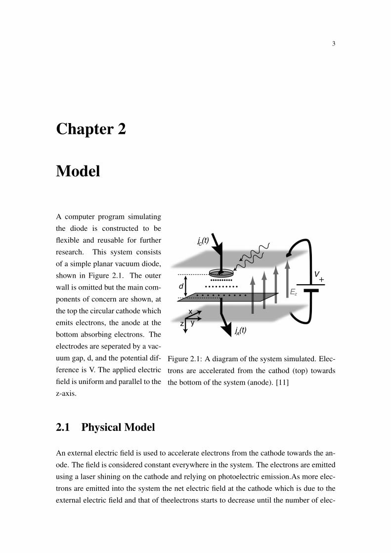
Figure 2.1: A diagram of the system simulated. Elec-trons are accelerated from the cathod (top) towardsthe bottom of the system (anode). [11]
A computer program simulatingthe diode is constructed to beflexible and reusable for furtherresearch. This system consistsof a simple planar vacuum diode,shown in Figure 2.1. The outerwall is omitted but the main com-ponents of concern are shown, atthe top the circular cathode whichemits electrons, the anode at thebottom absorbing electrons. Theelectrodes are seperated by a vac-uum gap, d, and the potential dif-ference is V. The applied electricfield is uniform and parallel to thez-axis.
2.1 Physical Model
An external electric field is used to accelerate electrons from the cathode towards the an-ode. The field is considered constant everywhere in the system. The electrons are emittedusing a laser shining on the cathode and relying on photoelectric emission.As more elec-trons are emitted into the system the net electric field at the cathode which is due to theexternal electric field and that of theelectrons starts to decrease until the number of elec-

4 High resolution simulation of a vacuum microdiode
trons emitted is great enough to reverse the field where electrons are emitted. Emission isspace-charge limited meaning that emission continues until enough electrons are emittedso that the net electric force at the cathode becomes zero. Another option is to have theemission source limited. That way there is a limit of available electrons released at thecathode in each iteration and only N electrons can be emitted at each iteration. This thesisis concerned with the space-charge limited regime.
2.2 Computational Algorithm
Since the program is to be used as a research tool for other people it needs to be clearlywritten and easy to understand so it can easily be run for other scenarios. Algorithm 1shows a pesudo code of how it is constructed. The implementation of these functions isnot shown but explained in later chapters.
Algorithm 1 Flow of the programInitialize program variableswhile (Conditions true) do
Add electrons to systemCalculate forces in systemMove electronsCheck boundary conditionsSave data (Positioning at each iteration) [Optional - Potentially slow]
end whileSave data (Escape vectors)
C++ was chosen for the simulation and Python for the data analysis.
The easiest way to program was to create a class with vectors which keep track of po-sitions, escaped electrons and force, to name a few parameters, and all functions belongto this class. Thus calling a function to move the electrons is easy and there is no needto supplement any variables to the function. This means that all functions and variablesof this class can be accessed by using the dot operator. Usually functions are seperateentities and have to be supplemented with input variables and return output variables butusing the class method complex functions which require much input data are extremelysimple to call.
Pálmar Jónsson 5
2.2.1 Emission
Random Distribution Algorithm
Normally a program like this has a huge number of particles and needs sophisticated ran-dom number generating algorithm which produces a long sequence of apparently randomresults. In this simulation the number of electrons is so small that almost any algorithmshould do. The one used is from technical enhancements to the C++ library and resultsshown in Figure 2.2 are considered adequate proof of quality. The one used is a versionof „Add-with-carry” with period likely in the range 10200 to 10500 [7]. If a larger period isneeded the „Mersenne Twister” (mt19937) algorithm has a period of 219937 − 1 [?] and iswidely used in computer simulations. A PIC simulation can have from 103 to 106 particles[3] while in this thesis the number of electrons in the system at any given iteration wasalways < 103.
Circular Distribution
When injecting electrons into the system they’re placed randomly on a circle with radiusof 250[nm] and 1[nm] below the surface of the cathode. This is done by choosing tworandom numbers from a uniform distribution, one corresponding to radius and the otherto angle. To make sure that the area distribution is the same everywhere on the cathodecare must be taken when assigning the raidal position. Each radial segment extendingfrom ri to ri+1 must be of the same size as any other. Thus
∫ r1
r0
∫ 2·π
0r · dr · dθ =
∫ r2
r1
∫ 2·π
0r · dr · dθ (2.1)
and subsequently
r22 = 2 · r2
1 − r20
r23 = 2 · r2
2 − r21.
(2.2)
By continuing with this method and realizing that r0 is just the center, equal to zero, aformula for the n-th radius is given by
r2n = n · r2
1 (2.3)
6 High resolution simulation of a vacuum microdiode
Another observation is that rN is the outer radius of the emitter, equal to 250[nm] in thiscase. Thus
r1 =rN√N
(2.4)
Substituting Equation (2.4) into Equation (2.3) and using the knowledge that rN = 250[nm]
gives
rn =
√n√N· 250[nm] n = 1, 2, ..., N − 1, N. (2.5)
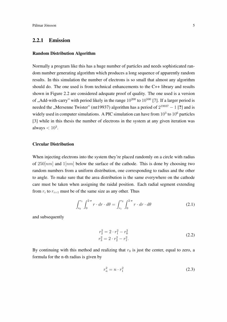
Figure 2.2: Distribution of electrons over theCathode at the first iteration. Cathode sur-face shown as circle.
The fraction above, n/N , is a random vari-able in the interval [0, 1] which is chosenfrom a uniform random distribution andthe square root taken of that number andthat is the radius used. This method en-sures that the area density of electrons isconstant everywhere on the surface of thecathode. Figure 2.2 shows the view of thex-y plane after first iteration as well as aoutline of the surface of the cathode.
With the radial length calculated the angu-lar position is a random number uniformlydistributed in the range [0, 360].
Initial Positioning
When injecting a new electron into the sys-tem a random position is generated in the x-y plane. Then the electron is placed 1[nm]
below the surface of the diode, at z-position −1[nm], and the forces which act upon eachelectron are calculated. If the sum of the forces act in the positive z-direction, so that theelectron is accelerated into the system, then she is injected at z-position of 1[nm]. Other-wise she’s removed and the process starts again until 100 unsuccessful attempts in a roware registered. Then the cathode is considered saturated and the system is evolved onetimestep. If an electron has 99 failed attempts but is successfully injected at attempt 100then this counter is reset to zero. That is the counter is not cumulative for all electrons.The reason why 1[nm] is chosen is that the cathode is considered to have some thicknessand 1[nm] to be the surface of the cathode.

Pálmar Jónsson 7
Initial Velocity and Movement Equation
Note that this part uses Equation (2.25) introduced later, Section 2.2.3.The equation for movement, Equation (2.25), uses position xi and xi−1 to calculate po-sition xi+1. When electrons are injected position xi−1 doesn’t exist for the injected elec-trons to calculate position xi+1. By setting this position to x = 0 the elctron wouldhave considerable initial velocity and zero if the same position would be used for xi−1 asfor xi. Equation (2.25) is presented here to help understanding the thought behind thismethod
xi+1 = xi +xi − xi−1
∆t· (∆t) +
F
m· (∆t)2. (2.6)
The middle term determines the initial velocity and by choosing xi−1 the initial velocitycan be chosen at will.The kinetic energy of an electron travelling through the system can be stated directly interms of the voltage applied. If the voltage is 2[V ] the maximum energy of an electrongoing from the cathode to the anode is equal toE = 2[eV ] [9]. The program can calculatea position, xi−1, so that any percentage of this maximum energy can be chosen as initialenergy. The derivations follows. The equation for kinectic energy is
E =1
2·m · v2 (2.7)
where E and m are known values. Then
v =
√2 · Em
. (2.8)
The velocity is calculated from current and former position and the timestep which canbe written as
v =xi − xi−1
∆t(2.9)
and by substituting Equation (2.9) in Equation (2.8) and simplifying the result is
xi−1 = xi −√
2 · Em·∆t (2.10)
where all the variable on the right side are known, xi being the newly calculated positionon the cathode.
Equation (2.10) isn’t yet in its final form. In this form each electron would have the sameinitial speed but to introduce initial speed some modifications has to be done, adding a
8 High resolution simulation of a vacuum microdiode
random factor to the initial speed. There are two ways of doing this having either uniformenergy distribution or uniform velocity distribution.
Equation (2.11) shows the uniform velocity distribution,
xi−1 = xi −√
2 · Em·∆t ·Random_Uniform(0, 1). (2.11)
Equation (2.12) shows the uniform energy distribution,
xi−1 = xi −√
2 · E ·RandUniform(0, 1)
m·∆t. (2.12)
Temperature and Initial Velocity
The temperature of the system plays a vital role in simulations. The Boltzmann distri-bution gives the energy of a system as k · T . For electrons to be emitted with 1% of themaximum final kinetic energy the temperature of the system can be estimated by
k · T = KE (2.13)
where k is the Boltzmann constant in[eVK
], K is the temperature of the system in [K] and
KE is the fraction of the maximum final energy in [eV ]. Putting in values for h and KEand solving for T the temperature is
T =0.01[eV ]
8.62 · 10−5[eV/K]= 116[K]. (2.14)
On the more familiar Celsius temperature scale this equals−157[◦C] so some kind of liq-uid cooling system would have to be used. If the diode were to be operated at room tem-perature of 20[◦C] then the maximum initial kinetic energy of the electrons is 0.48[eV ].Such an extreme scenario was not simulated. For comparison liquid Nitrogen has a boil-ing point of 77[K] (−196[◦C])
2.2.2 Force Calculation
There are two seperate forces acting upon electrons in the diode. One is due to staticelectric field and the other one is due to Coulumb forces between each electron and allother electrons in the system.
Pálmar Jónsson 9
Uniform External Electric Field
There is a fixed potential over the whole diode. This yields a electric field of
E =V
d, (2.15)
where d is the gap spacing and V the voltage at the anode.
This field affects the electrons in the system by linear relations,
F = q · E. (2.16)
Radial Electric Field
The code also permits the application of an externally applied radial electric field, butit is not used in this thesis. It must be calculated in conjunction with the axial field tosatisfy
5 ·D = 0. (2.17)
Coulumb Forces
The electric field due to a single electron is given by
~E =qe
4 · π · ε · r2r̂ (2.18)
where r is the distance to the point of measure.
The force acting upon another electron is
~F =q2e
4 · π · ε · r2r̂, (2.19)
which is the result of substituting Equation (2.18) into Equation (2.16).
In these equations ε = ε0·εr is the permittivity of the medium. Since vacuum is consideredto be inside the diode the relative permittivity, εr is equal to 1 and therefor ε = ε0. In theseequations r is the distance between two electrons given by
r =√
(∆x)2 + (∆y)2 + (∆z)2. (2.20)
10 High resolution simulation of a vacuum microdiode
The x,y and z components of the force are calculated by multiplying the force equationwith ∆x
rresulting in the following equation
Fx =q2e
4 · π · ε · r2· ∆x
r=
q2e · (x2 − x1)
4 · π · ε · [(x2 − x1)2 + (y2 − y1)2 + (z2 − z1)2]3/2(2.21)
which is used for the three Cartesian dimensions used in all calculations.
2.2.3 Equations of Motion
The Verlet algorithm is calculated using a Taylor expansion for position at time xt−∆t andxt+∆t and adding the equations and simplify [8, 4]
~xi+1 = ~xi + ~vi ·∆t+ ~ai·(∆t)22
+ Higher order terms~xi−1 = ~xi − ~vi ·∆t+ ~ai·(∆t)2
2∓ Higher order terms,
(2.22)
resulting inxi+1 = 2 · xi + vi · (∆t) + ai · (∆t)2. (2.23)
In this form the only variable which hasn’t been accounted for is the acceleration, a.Newton’s second law states that
F = m · a→ a =F
m(2.24)
where F was calculated by the methods shown in the force calculations section and mis the mass of an electron, me = 9.11 · 10−31[kg]. Substituting Equation (2.24) intoEquation (2.23) gives the form used in calculations of new position
xi+1 = 2 · xi − xi−1 +F
m· (∆t)2. (2.25)
2.2.4 Absorption
The only ways electrons are removed from the system is if they exceed the system bound-aries at cathode or anode. The system dimensions are assumed to be such that the sideshave no effect on the system and since the external electric field is considered uniformeverywhere in the anode they all escape at anode or cathode eventually.
Pálmar Jónsson 11
Anode
This is where the majority of electrons escape the system from. They cross the systemand are absorbed at the anode and that is the normal operation of the diode. The electronsaren’t absorbed instantaneously and the subchapter Section 2.2.5 discusses method usedto simulate absorption spread over time.
Cathode
A very small part of the electrons are pushed back into the cathode because of Coulumbforces. If an electron is tested at−1[nm] and injected into the system but when it’s placedon the surface of the cathode at 1[nm] it is possible that there is another electron extremlyclose to that position. This causes extreme Coulumb forces between these electrons push-ing the one closer to the cathode back into it. This is an extreme case and the total numberof electrons escaping this way is insignificant.
Both anode and cathode are considered perfectly flat.
12 High resolution simulation of a vacuum microdiode
2.2.5 Data Analysis
After a single simulation the following steps are taken in data analysis.
Acquisition
As shown in Algorithm 1 there are two ways to save the data. One method saves data aftereach iteration and keeps track of three dimensional position in CSV format. This makes itpossible to visualize the distribution after the first emission process to verify that the areadistribution is correct and also make a video of the system to see how it behaves. Thismethod is optional as accessing the hard disk drive in every iteration dramatically slowsdown simulations.The second method, which is run after the main program loop, saves one vector whichis as long as there are many iterations. Each element in this vector holds a count ofhow many electrons escape at each iteration. The index of the vector corresponds to theiteration at which the electrons escaped the system. Further discussion about how thisdata is used is in the Data Analysis chapter.
Filtering
The charge of the electrons isn’t absorbed by the boundaries all at once but spread overtime. A Gaussian smoothing curve is convoluted with the data to represent the charge be-ing absorbed over time. The only parameters of this smoothing function which need to bedetermined are the standard deviation of the curve, σ, and how wide the the curve shouldbe. Since about 99.7% of the data in a Gaussian distribution lies within three standarddeviations from the mean, the width of the smoothing function is chosen to be six timethe standard deviation and not changed for the remainder of this thesis. That equals threestandard deviations in each direction from the center which accounts for the 99.7%. Thissmoothing function is convoluted with the raw data for emission and absorption resultingin smooth curves. It should be noted that a wide smoothing function removes very highfrequency components from the signal but they’ve been observed to be mearly a fractionof the amplitude of the largest peaks which have always had frequencies which are lowerthan 2.5[THz]. The magnitude of the smoothing function is normalized to one althoughthat doesn’t result in the area of the distribution to equal one. The magnitude scale isarbitrary in this thesis and only the frequencies are of interest. Note that fourier analysisplots will show the x-axis go up to 2.5[THz] or [3.5[THz] but the different cutoffs arenot significant to the readers understanding of what’s happening in the figures.

Pálmar Jónsson 13
Figure 2.3: Gaussian bell curve to be convoluted with raw data
For the remainder of this thesis all data is smoothed using the following parameters,shown in Table 2.1, in the Gaussian smoothing function, Figure 2.3.
Emission AbsorptionValue Value Value Value
σ 800[iter] 800[fs] 400[iter] 400[fs]Total width 6 · σ (iter) 4800[fs] 400[iter] 2400[fs]
Table 2.1: Parameters for smoothing function
To justify the size of the filter the de Broglie wavelength and final velocity of an electronare calculated and the time it takes an electron to travel the distance of one de Brogliewavelength. The de Broglie wavelength is defined as [9, p. 1494]
λ[nm] =h
p=h · cp · c
(2.26)
where h · c ' 1240[eV · nm] and p · c =√
2 ·K ·m0 · c2 with K being the kineticenergy, m0 the mass of the electron and c the speed of light in vacuum. The reason formultiplying in Equation (2.26) is to get familiar and widely known values. Substitutionand simplification results in
λ[nm] =1.23[eV · nm]
K[eV ]. (2.27)
14 High resolution simulation of a vacuum microdiode
The final velocity of an electron in the system is given by
v =
√2 · e · ϕm
(2.28)
where ϕ is the voltage potential at the anode and e is the magnitude of the charge of anelectron. Realizing that ϕ = K, simplification results in
v = 59.310 ·√K[eV ][m/s]. (2.29)
Then the time, τ , it takes the electron to travel one de Broglie wavelength is
τ =λ
v=
1.23 · 10−9/√K[eV ]
59310 ·√K[eV ]
[m
m/s
]≈ 20
K[fs]. (2.30)
where K is in [eV ]. Thus we see that the value of σ only amounts to the time taken to spantens of de Broglie wavelengths whereas the frequenies observed correspond to periods atorder an magnitude greater than σ.
Fourier Analysis
The data from simulations is just a count of how many electrons escape in each iterationand is represented by integers. Since the charge of an electron absorbed by a metal sur-face isn’t absorbed all at once but over some time a Gaussian like smoothening functionis convoluted with the data to produce a graph of electrons absorbed at anode versus it-eration, which can be translated directly into time. This makes it possible to do a fourieranalysis on the data and determine the frequency components present in the signal. Aftermany iterations and tuning of the Fourier analysis it became apparent that no frequencies,of any importance, over 3.5[THz] are present so every graph of the fourier transformshows a frequency scale from zero to 3.5[THz]. This way the relevant data is easier toidentify.
The way the data is presented to the Fourier analysis if of great importance. If the datahas mean(x) > 0 then the the first value in the analysis will be large and quite possiblymuch larger than the actual frequencies present in the signal and can be thought of asa DC-component in the signal. To understand this the equation for the discrete FourierAnalysis is shown in Equation 2.31

Pálmar Jónsson 15
F [k] =N−1∑k=0
xn · e−i·2·π·kN·n k = 0, 1, ..., N − 2, N − 1 (2.31)
When calculating the first term, F [0], the exponent of e is always zero so the first valueis the sum of all values in the signal. To get rid of this unwanted behaviour the mean ofthe signal vector is subtracted from each value before applying the Fourier analysis so theresult shows the frequency components present in the signal but not this unwanted artifact.To further illustrate this point Figure 2.4 shows the difference between synthetic signalconstructed from two sinusoids with frequencies 10[Hz] and 23.75[Hz] plus a constantto simulate a mean larger than zero and white noise.
Figure 2.4: Fourier comparison
A built in function of the Numpy package[1] was used to calculate the transform while thefrequency axis (x-axis) was built using as many elements as are present in the signal in therange from 0 to half the sampling frequency. The frequency component at 23.75[Hz] hasabout the same magnitude as the noise in the beginning of the signal but is much betterdefined as a peak. This is due to the way the signal is constructed where the sinusoid withthe higher frequency has much lower amplitude that the lower frequency component.Therefor the magnitude of the noise in the signal is comparable to the low amplitudefrequency component although the shape of the higher frequency component is muchmore definite.

16
17
Chapter 3
Results
Many different combinations of the parameters V and D were simulated but the casewhere V = 1[V ] and D = 2[µm] will be presented to be able to compare results withresearch done earlier[11].
3.1 Emission
The emission process shows that the electron emission is somewhat clustered, almost asif there are sheets being discretely emitted. The reason for this is that in the beginning thesystem is almost empty (only empty for the first try) and Columb forces are negligible.After the system gets saturated it’s evolved one timestep and further emission is attempted.Until the first „sheet” of electrons has moved a certain distance away from the cathodeonly few electrons are emitted. Once the first sheet crosses this distance the net electricfield at the cathode acts in a direction so that more electrons are drawn into the systemgiving birth to the second sheet. After few iterations of this process the injection processstarts to take place over a wider range of iterations although it never comes close to beingso that it can be called continous, it is always pulsed. Figure 3.1 shows the raw data ofthe injected electrons.

18 High resolution simulation of a vacuum microdiode
Figure 3.1: Raw Emission Data
The beginning of Figure 3.1 shows an unusually large peak at iteration 0 and the x-axishas been modified so that this peak can be seen as data but not part of the frame ofthe figure. This is because there are no electrons in the system at the beginning andtherefor no blocking effects because of Coulumb forces by other electrons so a largenumber of electrons is emitted at the beginning. This behaviour does not continue in lateremissions.
The data resulting from convoluting the emitted data with the Gaussian smoothing func-tion is shown in Figure 3.2. The figure’s x-axis is changed to show the first iteration moreclearly.
Pálmar Jónsson 19
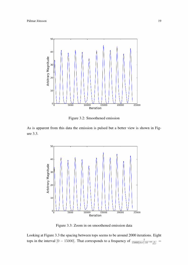
Figure 3.2: Smoothened emission
As is apparent from this data the emission is pulsed but a better view is shown in Fig-ure 3.3.
Figure 3.3: Zoom in on smoothened emission data
Looking at Figure 3.3 the spacing between tops seems to be around 2000 iterations. Eighttops in the interval [0 − 15000]. That corresponds to a frequency of 7
15000[iter]·10−15 siter
=
20 High resolution simulation of a vacuum microdiode
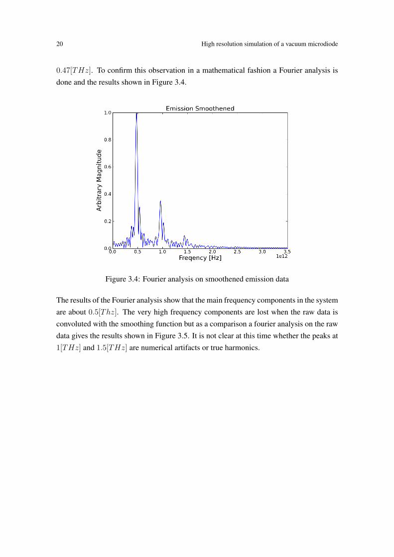
0.47[THz]. To confirm this observation in a mathematical fashion a Fourier analysis isdone and the results shown in Figure 3.4.
Figure 3.4: Fourier analysis on smoothened emission data
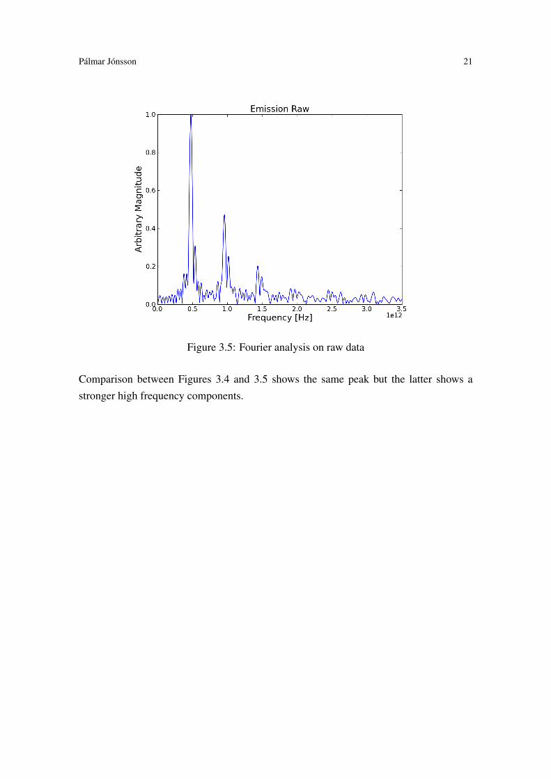
The results of the Fourier analysis show that the main frequency components in the systemare about 0.5[Thz]. The very high frequency components are lost when the raw data isconvoluted with the smoothing function but as a comparison a fourier analysis on the rawdata gives the results shown in Figure 3.5. It is not clear at this time whether the peaks at1[THz] and 1.5[THz] are numerical artifacts or true harmonics.
Pálmar Jónsson 21
Figure 3.5: Fourier analysis on raw data
Comparison between Figures 3.4 and 3.5 shows the same peak but the latter shows astronger high frequency components.

22 High resolution simulation of a vacuum microdiode
3.2 Absorption
Although the emission process shows that the system behaves the way it is expected itdoesn’t really matter so much for the function of the diode. The absorption howevershows whether the diode could be useful as a high frequency generator. Figure 3.6 showsa zoom in on the smoothened absorped data.
The first peak of Figure 3.1 doesn’t show up as data has been discarded so that the fluctua-tions in the beginning don’t show up in the analysis of the steady state of the diode.
Figure 3.6: Absorped smoothened data
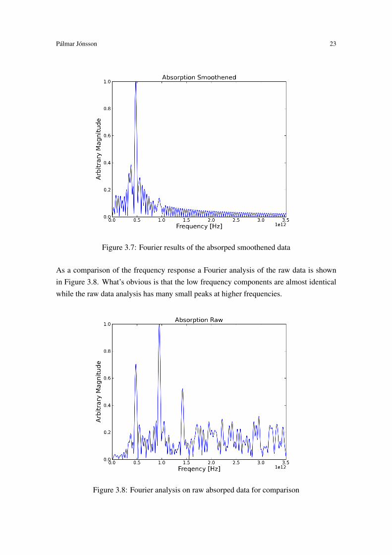
Fourier analysis of this data shows the frequencies present in the signal. Figure 3.7 showsa dominant frequency at ≈ 0.5[THz] and smaller spikes around it. The ratio of thedominant frequency against the second highest is 2.6 whether the data presented is useddirectly or an upper envelope constructed and analyzed. The width is 0.049[THz] to0.093[THz], centered around 0.48[THz].
Pálmar Jónsson 23
Figure 3.7: Fourier results of the absorped smoothened data
As a comparison of the frequency response a Fourier analysis of the raw data is shownin Figure 3.8. What’s obvious is that the low frequency components are almost identicalwhile the raw data analysis has many small peaks at higher frequencies.
Figure 3.8: Fourier analysis on raw absorped data for comparison

24 High resolution simulation of a vacuum microdiode
The difference between Figure 3.7 and Figure 3.8 is that the frequency components at1[THz] and 1.5[THz] which are strong in Figure 3.8 get smoothened and are not presentin the analysis on the filtered data, Figure 3.7.
Pálmar Jónsson 25
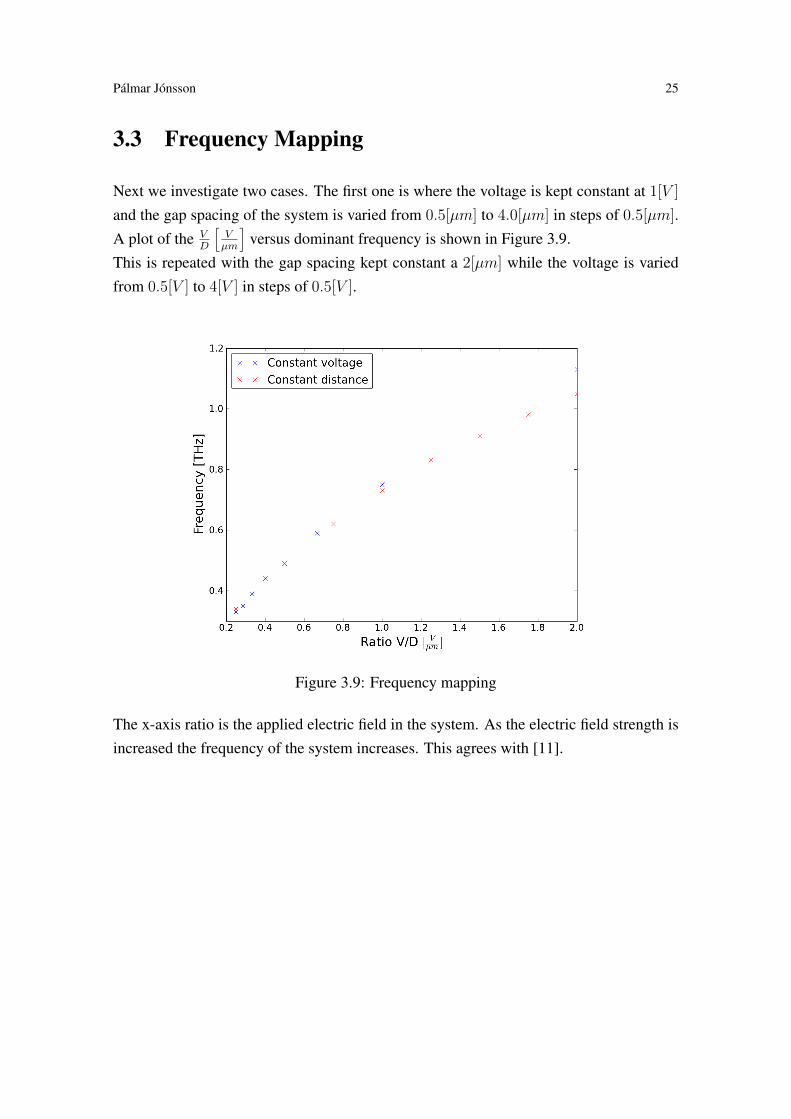
3.3 Frequency Mapping
Next we investigate two cases. The first one is where the voltage is kept constant at 1[V ]
and the gap spacing of the system is varied from 0.5[µm] to 4.0[µm] in steps of 0.5[µm].A plot of the V
D
[Vµm
]versus dominant frequency is shown in Figure 3.9.
This is repeated with the gap spacing kept constant a 2[µm] while the voltage is variedfrom 0.5[V ] to 4[V ] in steps of 0.5[V ].
Figure 3.9: Frequency mapping
The x-axis ratio is the applied electric field in the system. As the electric field strength isincreased the frequency of the system increases. This agrees with [11].
26 High resolution simulation of a vacuum microdiode
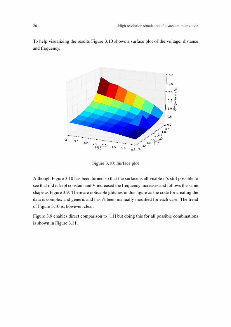
To help visualizing the results Figure 3.10 shows a surface plot of the voltage, distanceand frequency.
Figure 3.10: Surface plot
Although Figure 3.10 has been turned so that the surface is all visible it’s still possible tosee that if d is kept constant and V increased the frequency increases and follows the sameshape as Figure 3.9. There are noticable glitches in this figure as the code for creating thedata is complex and generic and hasn’t been manually modified for each case. The trendof Figure 3.10 is, however, clear.
Figure 3.9 enables direct comparison to [11] but doing this for all possible combinationsis shown in Figure 3.11.
Pálmar Jónsson 27
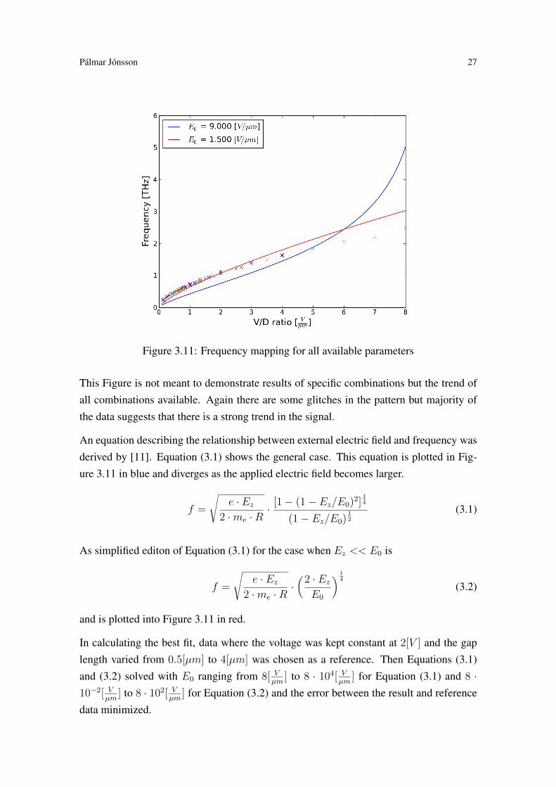
Figure 3.11: Frequency mapping for all available parameters
This Figure is not meant to demonstrate results of specific combinations but the trend ofall combinations available. Again there are some glitches in the pattern but majority ofthe data suggests that there is a strong trend in the signal.
An equation describing the relationship between external electric field and frequency wasderived by [11]. Equation (3.1) shows the general case. This equation is plotted in Fig-ure 3.11 in blue and diverges as the applied electric field becomes larger.
f =
√e · Ez
2 ·me ·R· [1− (1− Ez/E0)2]
14
(1− Ez/E0)12
(3.1)
As simplified editon of Equation (3.1) for the case when Ez << E0 is
f =
√e · Ez
2 ·me ·R·(
2 · EzE0
) 14
(3.2)
and is plotted into Figure 3.11 in red.
In calculating the best fit, data where the voltage was kept constant at 2[V ] and the gaplength varied from 0.5[µm] to 4[µm] was chosen as a reference. Then Equations (3.1)and (3.2) solved with E0 ranging from 8[ V
µm] to 8 · 104[ V
µm] for Equation (3.1) and 8 ·
10−2[ Vµm
] to 8 · 102[ Vµm
] for Equation (3.2) and the error between the result and referencedata minimized.

28 High resolution simulation of a vacuum microdiode
For the general case the plot diverges (blue curve) which was the result of [11]. Theresults show that when the applied electric field is weak the plot of Equation (3.2) followsthe simulated data very closely (red curve).
Pálmar Jónsson 29
3.4 Initial Velocity (5%)
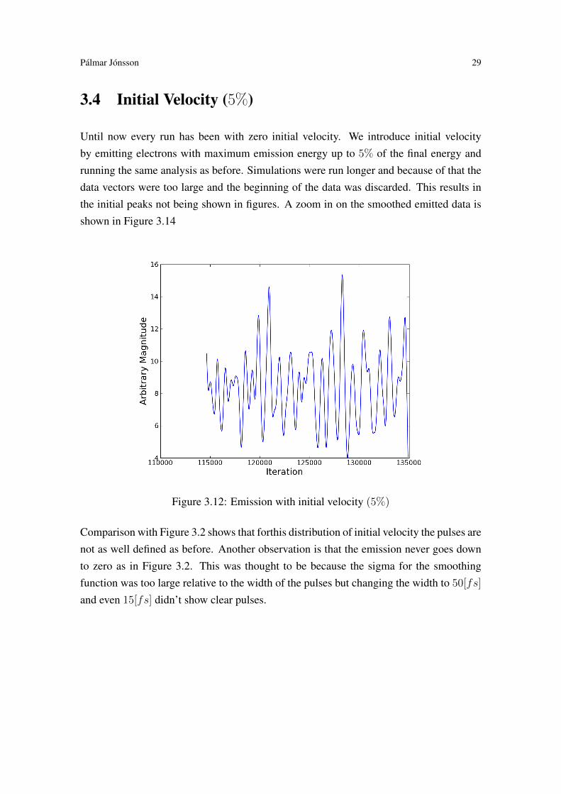
Until now every run has been with zero initial velocity. We introduce initial velocityby emitting electrons with maximum emission energy up to 5% of the final energy andrunning the same analysis as before. Simulations were run longer and because of that thedata vectors were too large and the beginning of the data was discarded. This results inthe initial peaks not being shown in figures. A zoom in on the smoothed emitted data isshown in Figure 3.14
Figure 3.12: Emission with initial velocity (5%)
Comparison with Figure 3.2 shows that forthis distribution of initial velocity the pulses arenot as well defined as before. Another observation is that the emission never goes downto zero as in Figure 3.2. This was thought to be because the sigma for the smoothingfunction was too large relative to the width of the pulses but changing the width to 50[fs]
and even 15[fs] didn’t show clear pulses.
30 High resolution simulation of a vacuum microdiode
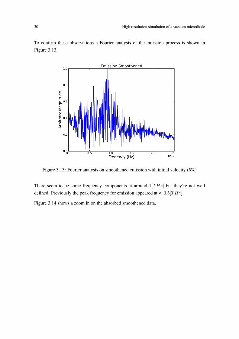
To confirm these observations a Fourier analysis of the emission process is shown inFigure 3.13.
Figure 3.13: Fourier analysis on smoothened emission with initial velocity (5%)
There seem to be some frequency components at around 1[THz] but they’re not welldefined. Previously the peak frequency for emission appeared at ≈ 0.5[THz].
Figure 3.14 shows a zoom in on the absorbed smoothened data.

Pálmar Jónsson 31
Figure 3.14: Absorption with initial velocity (5%)
Again comparison with the results without initial velocity, Figure 3.6, shows much worsepulsing, if any. The x-axis scaling is automatic resulting in a empty space in the beginningbut that has no effects on the analysis.
32 High resolution simulation of a vacuum microdiode
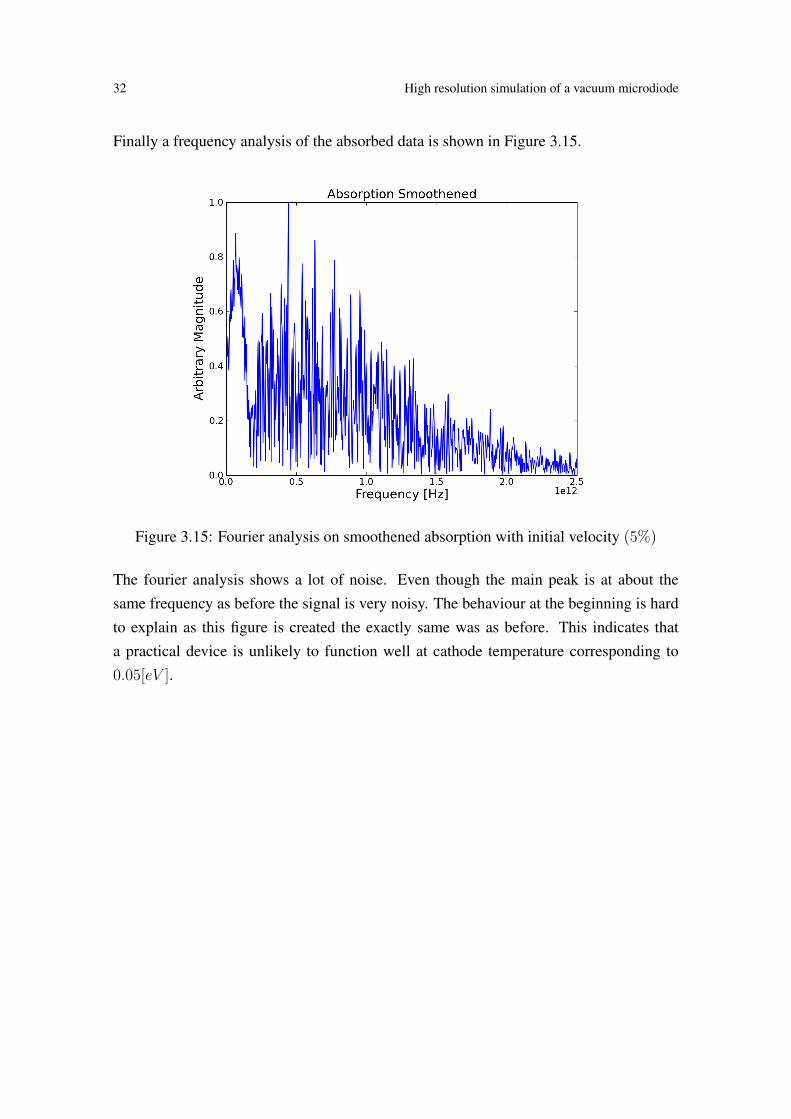
Finally a frequency analysis of the absorbed data is shown in Figure 3.15.
Figure 3.15: Fourier analysis on smoothened absorption with initial velocity (5%)
The fourier analysis shows a lot of noise. Even though the main peak is at about thesame frequency as before the signal is very noisy. The behaviour at the beginning is hardto explain as this figure is created the exactly same was as before. This indicates thata practical device is unlikely to function well at cathode temperature corresponding to0.05[eV ].
Pálmar Jónsson 33
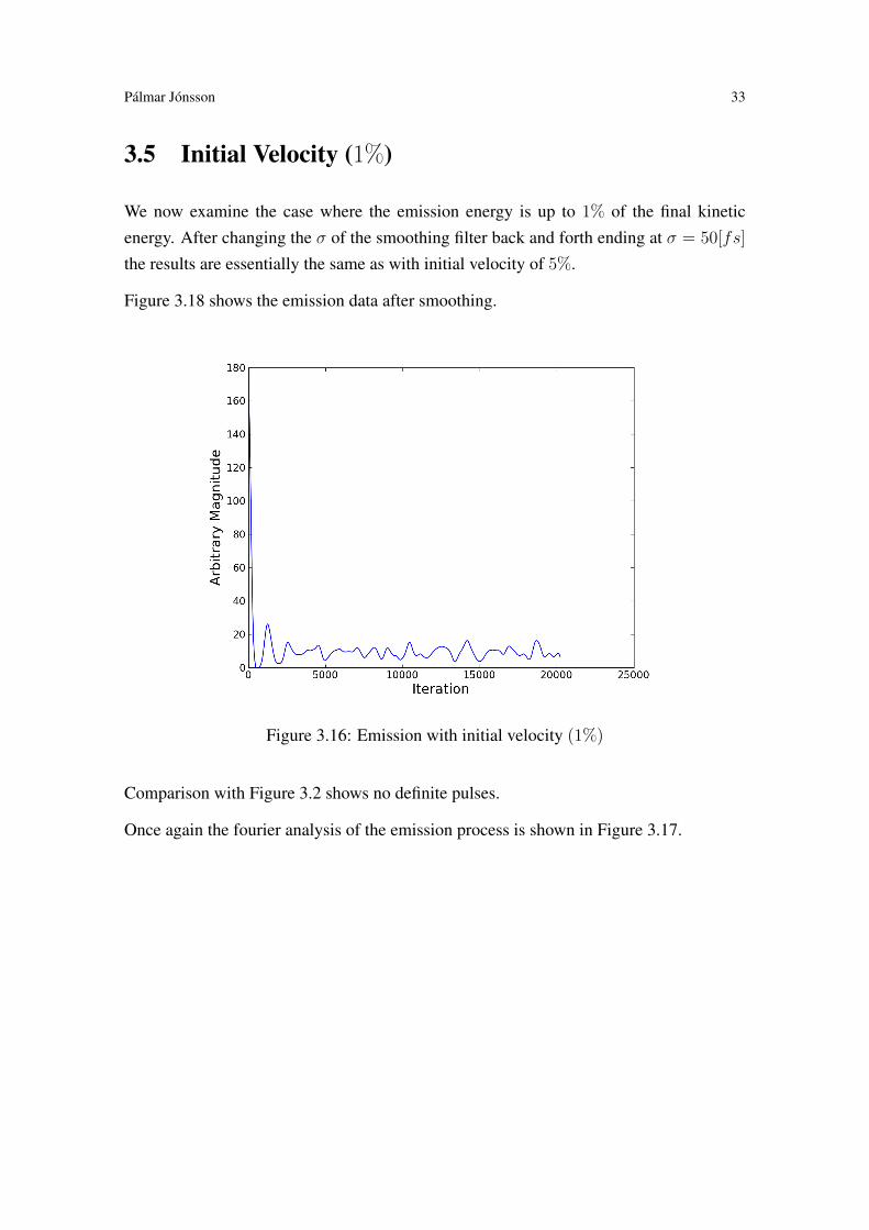
3.5 Initial Velocity (1%)
We now examine the case where the emission energy is up to 1% of the final kineticenergy. After changing the σ of the smoothing filter back and forth ending at σ = 50[fs]
the results are essentially the same as with initial velocity of 5%.
Figure 3.18 shows the emission data after smoothing.
Figure 3.16: Emission with initial velocity (1%)
Comparison with Figure 3.2 shows no definite pulses.
Once again the fourier analysis of the emission process is shown in Figure 3.17.
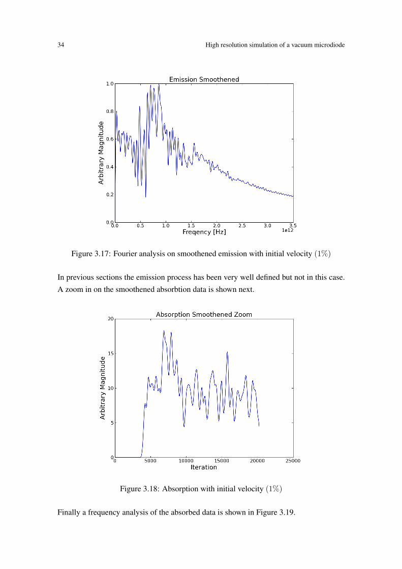
34 High resolution simulation of a vacuum microdiode
Figure 3.17: Fourier analysis on smoothened emission with initial velocity (1%)
In previous sections the emission process has been very well defined but not in this case.A zoom in on the smoothened absorbtion data is shown next.
Figure 3.18: Absorption with initial velocity (1%)
Finally a frequency analysis of the absorbed data is shown in Figure 3.19.

Pálmar Jónsson 35
Figure 3.19: Fourier analysis on smoothened absorption with initial velocity (1%)
It’s hard to see whether this shows a low frequency component or if the absorption isbecoming continuous.
Final Remarks
It’s hard to simulate every physical aspect of microdiodes and simplifications have to bedone and have been in the past with methods such as PIC. This thesis explored the be-haviour of a vacuum microdiode with and without initial velocity and confirmed earlierresearch [11] using the same assumptions and restrictions. Attempts to go further and mapparameters as well as removing certain restrictions on the initial system were made withlittle success. Further research into vacuum microdiodes with initial velocity is neededas well as better understanding of the way an electron is absorped into the anode. Addi-tionally it seems that the diode would have to be cooled to minimize the effects of initialvelocity.
With computers becoming more powerful an extremely accurate simulation of micro-scopic physical systems is possible. The most computationally expensive component ofthe simulation is the Coulumb force calculation which was parallellized and run on a IntelCore i7 processor but can be run in larger clusters of computers. Although this kind ofsimulation would benefit more using a faster processor than many cores as the number ofelectrons in the system at any given time was small.

36

37
Bibliography
[1] David Ascher, Paul F. Dubois, Konrad Hinsen, James Hugunin, and Travis Oliphant.Numerical Python. Lawrence Livermore National Laboratory, Livermore, CA, ucrl-ma-128569 edition, 1999.
[2] R.J. Barker, IEEE Nuclear, and Plasma Sciences Society. Modern microwave and
millimeter-wave power electronics. IEEE Press, 2005.
[3] C.K. Birdsall. Particle-in-cell charged-particle simulations, plus monte carlo colli-sions with neutral atoms, pic-mcc. IEEE Transactions on Plasma Science, 1991.
[4] Jonathan Dummer. . [online] http://lonesock.net/article/verlet.html.
[5] J.A. Eichmeier and M. Thumm. Vacuum Electronics: Components and Devices.Springer, 2010.
[6] Particle in Cell Consulting LLC. The Electrostatic Particle In Cell (ES-PIC) Method, 2010. [online] http://www.particleincell.com/2010/es-pic-method/.
[7] Mathcom Solutions Inc. , 1995. [online] http://www.mathcom.com/
corpdir/techinfo.mdir/q210.html#q210.6.2.
[8] Wikimedia Foundation Inc. . [online] http://en.wikipedia.org/wiki/Verlet_integration.
[9] H.D. Young, R.A. Freedman, and A.L. Ford. Sears and Zemansky’s University
Physics: With Modern Physics. MasteringPhysics Series. Pearson Addison Wes-ley, 2004.
[10] W. Zhu. Vacuum Microelectronics. Wiley, 2001.

38 High resolution simulation of a vacuum microdiode
[11] Andreas Pedersen. Andrei Manolescu. Ágúst Valfells. Space-charge modulation invacuum microdiodes at thz frequencies. The American Physical Society - Physical
Review Letters, April 2010.
39
Appendix A
Program options
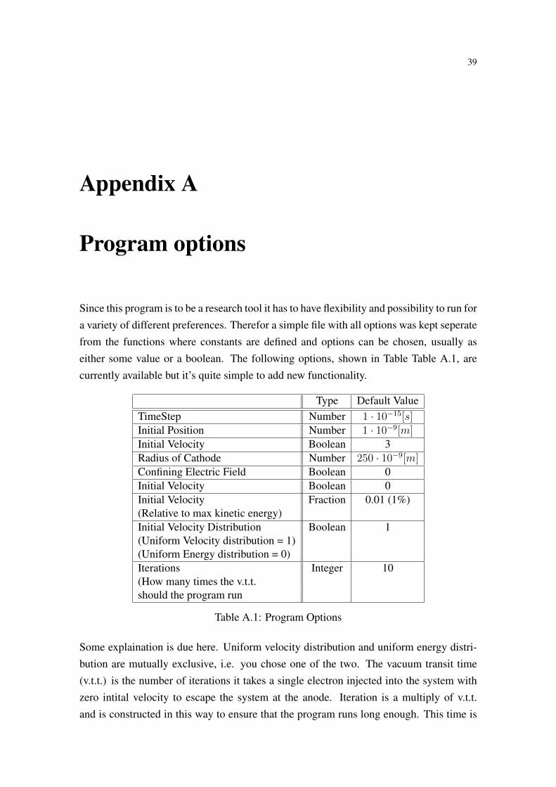
Since this program is to be a research tool it has to have flexibility and possibility to run fora variety of different preferences. Therefor a simple file with all options was kept seperatefrom the functions where constants are defined and options can be chosen, usually aseither some value or a boolean. The following options, shown in Table Table A.1, arecurrently available but it’s quite simple to add new functionality.
Type Default ValueTimeStep Number 1 · 10−15[s]Initial Position Number 1 · 10−9[m]Initial Velocity Boolean 3Radius of Cathode Number 250 · 10−9[m]Confining Electric Field Boolean 0Initial Velocity Boolean 0Initial Velocity Fraction 0.01 (1%)(Relative to max kinetic energy)Initial Velocity Distribution Boolean 1(Uniform Velocity distribution = 1)(Uniform Energy distribution = 0)Iterations Integer 10(How many times the v.t.t.should the program run
Table A.1: Program Options
Some explaination is due here. Uniform velocity distribution and uniform energy distri-bution are mutually exclusive, i.e. you chose one of the two. The vacuum transit time(v.t.t.) is the number of iterations it takes a single electron injected into the system withzero intital velocity to escape the system at the anode. Iteration is a multiply of v.t.t.and is constructed in this way to ensure that the program runs long enough. This time is
40 High resolution simulation of a vacuum microdiode
larger than in reality as Columb forces from electrons act to accelerate the first electronso that she escapes before this calculated v.t.t. iterations comes. It is possible though touse this as an rough estimate of how many „sheets” go through the system. Choosing 10for the „Iterations” we can assume that about 10 sheets are emitted and travel through thesystem.


School of Science and EngineeringReykjavík UniversityMenntavegur 1101 Reykjavík, IcelandTel. +354 599 6200Fax +354 599 6201www.reykjavikuniversity.isISSN 1670-8539


