Higher Radix Floating-Point Representations for FPGA-Based ...

HIGHER RADIX FLOATING-POINT REPRESENTATIONS FOR

FPGA-BASED ARITHMETIC

by

Bryan C. Catanzaro

A thesis submitted to the faculty of

Brigham Young University

in partial fulfillment of the requirements for the degree of

Master of Science

Department of Electrical and Computer Engineering

Brigham Young University

August 2005

Copyright c© 2006 Bryan C. Catanzaro

All Rights Reserved

BRIGHAM YOUNG UNIVERSITY

GRADUATE COMMITTEE APPROVAL

of a thesis submitted by

Bryan C. Catanzaro

This thesis has been read by each member of the following graduate committee andby majority vote has been found to be satisfactory.

Date Brent E. Nelson, Chair

Date Michael J. Wirthlin

Date Doran K. Wilde

BRIGHAM YOUNG UNIVERSITY

As chair of the candidate’s graduate committee, I have read the thesis of Bryan C.Catanzaro in its final form and have found that (1) its format, citations, and bibli-ographical style are consistent and acceptable and fulfill university and departmentstyle requirements; (2) its illustrative materials including figures, tables, and chartsare in place; and (3) the final manuscript is satisfactory to the graduate committeeand is ready for submission to the university library.

Date Brent E. NelsonChair, Graduate Committee

Accepted for the Department

Michael A. JensenGraduate Coordinator

Accepted for the College

Douglas M. ChabriesDean, Ira A. Fulton Collegeof Engineering and Technology

ABSTRACT

HIGHER RADIX FLOATING-POINT REPRESENTATIONS FOR

FPGA-BASED ARITHMETIC

Bryan C. Catanzaro

Department of Electrical and Computer Engineering

Master of Science

Field Programmable Gate Arrays (FPGAs) are increasingly being used for

high-throughput floating-point computation. It is forecasted that by 2009, FPGAs

will provide an order of magnitude greater sustained floating-point throughput than

conventional processors [1]. FPGA implementations of floating-point operators have

historically been designed to use binary floating-point representations, as do general

purpose processors. Binary representations were chosen as the standard over three

decades ago because they provide maximal numerical accuracy per bit of floating-

point data. However, the unique nature of FPGA-based computation makes numeri-

cal accuracy per unit of FPGA resources a more important measure of the usefulness

of a given floating-point representation.

From this viewpoint, higher radix floating-point representations are well suited

to FPGA-based computations, especially high precision calculations which require the

support of denormalized numbers. This work shows that higher radix representations

lead to more efficient use of FPGA resources. For example, a hexadecimal floating-

point adder provides a 30% lower Area-Time product than its binary counterpart,

and a hexadecimal floating-point multiplier has a 13% lower Area-Time product than

its binary counterpart. This savings occurs while still delivering equal worst-case

and better average-case numerical accuracy. This work presents a family of higher

radix floating-point representations that are designed specifically to interoperate with

standard IEEE floating-point, allowing the creation of floating-point datapaths which

operate on standard binary floating-point data, yet use higher radix representations

internally. Such datapaths provide higher performance by any measure: they are

more accurate numerically, consume less FPGA resources and have shorter laten-

cies. When taking into consideration the unique nature of FPGA-based computing

systems, this work shows that binary floating-point representations are not optimal

for most FPGA-based arithmetic computations. Higher radix representations can

therefore be a useful tool for building efficient custom floating-point datapaths on

FPGAs.

Contents

List of Tables xv

List of Figures xviii

1 Introduction 1

2 Background 5

2.1 Mathematical Terminology . . . . . . . . . . . . . . . . . . . . . . . . 5

2.2 Floating-Point Format Background . . . . . . . . . . . . . . . . . . . 8

2.2.1 IEEE Format Details . . . . . . . . . . . . . . . . . . . . . . . 8

2.2.2 Rounding . . . . . . . . . . . . . . . . . . . . . . . . . . . . . 10

2.2.3 Treatment of Special Numbers . . . . . . . . . . . . . . . . . . 11

2.2.4 Quadruple Precision . . . . . . . . . . . . . . . . . . . . . . . 12

2.3 Historical Background . . . . . . . . . . . . . . . . . . . . . . . . . . 14

2.4 On the Need for Bit-Identical Results . . . . . . . . . . . . . . . . . . 17

2.5 Related Work . . . . . . . . . . . . . . . . . . . . . . . . . . . . . . . 18

2.5.1 Floating-Point Arithmetic on FPGAs . . . . . . . . . . . . . . 18

2.5.2 Higher Radix Floating-Point Implementations . . . . . . . . . 20

3 Proposed Representation 23

3.1 Overview . . . . . . . . . . . . . . . . . . . . . . . . . . . . . . . . . . 23

3.2 Radix Point Position . . . . . . . . . . . . . . . . . . . . . . . . . . . 23

3.3 Encoding . . . . . . . . . . . . . . . . . . . . . . . . . . . . . . . . . 28

3.4 Flag Bits . . . . . . . . . . . . . . . . . . . . . . . . . . . . . . . . . . 31

3.5 Dynamic Range . . . . . . . . . . . . . . . . . . . . . . . . . . . . . . 32

xiii

3.6 Numerical Accuracy . . . . . . . . . . . . . . . . . . . . . . . . . . . 35

3.6.1 Worst Case Relative Error . . . . . . . . . . . . . . . . . . . . 35

3.6.2 Relative Significance Space Density . . . . . . . . . . . . . . . 37

3.6.3 Gap Functions . . . . . . . . . . . . . . . . . . . . . . . . . . 40

3.7 Rounding Procedures . . . . . . . . . . . . . . . . . . . . . . . . . . . 44

3.8 Summary . . . . . . . . . . . . . . . . . . . . . . . . . . . . . . . . . 46

4 Implementation 47

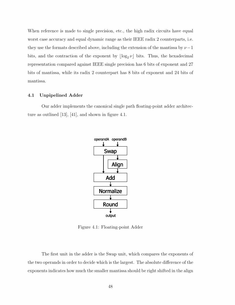
4.1 Unpipelined Adder . . . . . . . . . . . . . . . . . . . . . . . . . . . . 48

4.2 Unpipelined Multiplication . . . . . . . . . . . . . . . . . . . . . . . . 52

4.3 Converter Hardware . . . . . . . . . . . . . . . . . . . . . . . . . . . 56

4.4 Pipelined Operators . . . . . . . . . . . . . . . . . . . . . . . . . . . . 57

4.5 Floating-Point Unit Building Blocks . . . . . . . . . . . . . . . . . . . 60

4.5.1 Priority Encoder . . . . . . . . . . . . . . . . . . . . . . . . . 60

4.5.2 Normalizing and Aligning Shifters . . . . . . . . . . . . . . . . 60

4.6 Future Work . . . . . . . . . . . . . . . . . . . . . . . . . . . . . . . . 64

5 Conclusions 65

A Reducing Embedded Multiplier Usage 69

A.1 Justification . . . . . . . . . . . . . . . . . . . . . . . . . . . . . . . . 69

A.2 Factorization . . . . . . . . . . . . . . . . . . . . . . . . . . . . . . . 71

A.3 Architecture . . . . . . . . . . . . . . . . . . . . . . . . . . . . . . . . 72

A.4 Implementation . . . . . . . . . . . . . . . . . . . . . . . . . . . . . . 78

Bibliography 86

xiv

List of Tables

2.1 Round Logic . . . . . . . . . . . . . . . . . . . . . . . . . . . . . . . . 11

2.2 Special Numbers . . . . . . . . . . . . . . . . . . . . . . . . . . . . . 11

2.3 Addition Special Cases . . . . . . . . . . . . . . . . . . . . . . . . . . 13

2.4 Subtraction Special Cases . . . . . . . . . . . . . . . . . . . . . . . . 13

2.5 Multiplication Special Cases . . . . . . . . . . . . . . . . . . . . . . . 13

2.6 Division Special Cases . . . . . . . . . . . . . . . . . . . . . . . . . . 13

3.1 Encoded Numbers in Different Representations . . . . . . . . . . . . . 29

3.2 Floating-point Word Size with Equalized Numeric Performance . . . . 30

3.3 Standard Special Case Logic . . . . . . . . . . . . . . . . . . . . . . . 31

3.4 Encoded Flags . . . . . . . . . . . . . . . . . . . . . . . . . . . . . . . 32

3.5 Format Parameters . . . . . . . . . . . . . . . . . . . . . . . . . . . . 34

3.6 Dynamic Range . . . . . . . . . . . . . . . . . . . . . . . . . . . . . . 34

4.1 Unpipelined Adder Area Comparison . . . . . . . . . . . . . . . . . . 51

4.2 Unpipelined Adder Timing Comparison . . . . . . . . . . . . . . . . . 51

4.3 Unpipelined Multiplier Area Comparison . . . . . . . . . . . . . . . . 55

4.4 Multiplier Timing Comparison . . . . . . . . . . . . . . . . . . . . . . 55

4.5 Converter Circuitry Area . . . . . . . . . . . . . . . . . . . . . . . . . 57

A.1 Multiplier Sizes . . . . . . . . . . . . . . . . . . . . . . . . . . . . . . 78

xv

xvi

List of Figures

2.1 Standard Floating-Point Formats . . . . . . . . . . . . . . . . . . . . 9

3.1 Externally Radix 2, Internally Radix 16 System . . . . . . . . . . . . 24

3.2 Exponent Mapping, δ′ = 1ν

. . . . . . . . . . . . . . . . . . . . . . . . 27

3.3 Exponent Mapping, δ′ = 0 . . . . . . . . . . . . . . . . . . . . . . . . 27

3.4 Floating-Point Format Size Increase versus Radix . . . . . . . . . . . 30

3.5 Relative Worst Case Accuracy versus FP Word Size . . . . . . . . . . 36

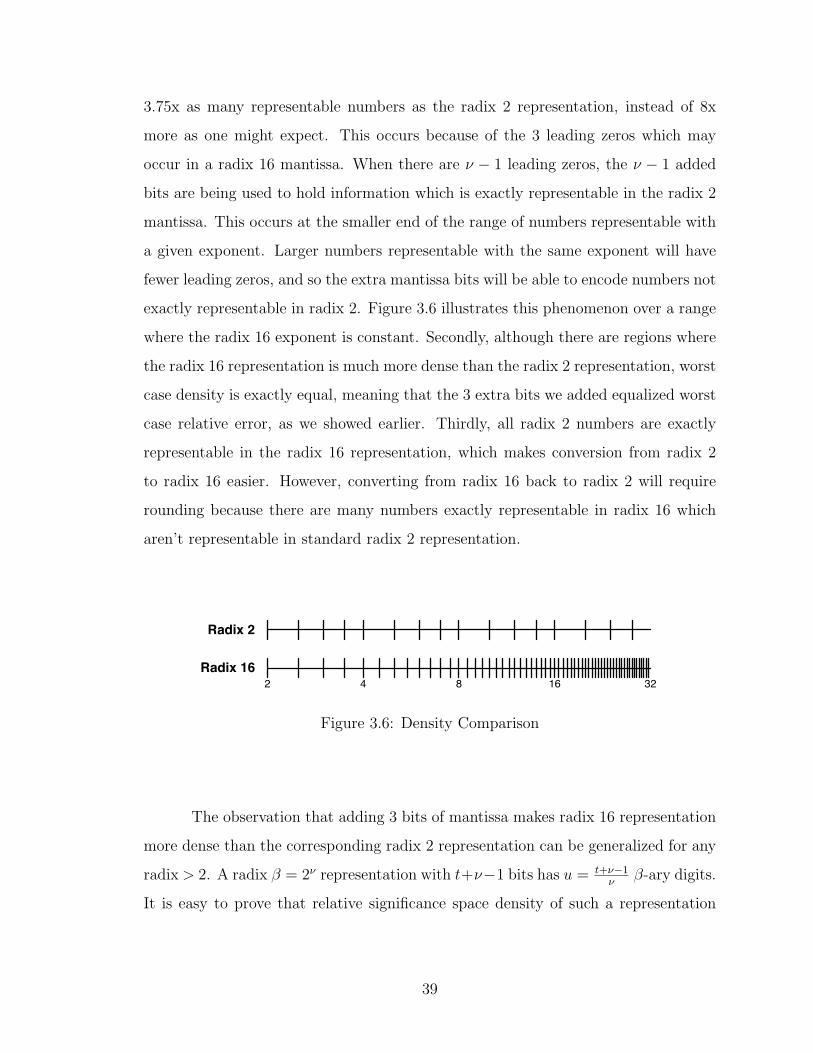
3.6 Density Comparison . . . . . . . . . . . . . . . . . . . . . . . . . . . 39

3.7 Relative Significance Space Density versus FP Word Size . . . . . . . 41

3.8 Gap functions for 32-bit Fixed-Point and 32-bit Floating-Point . . . . 42

3.9 Gap Functions for Radix 2 and Radix 16 Representations . . . . . . . 42

4.1 Floating-point Adder . . . . . . . . . . . . . . . . . . . . . . . . . . . 48

4.2 Area for Unpipelined Adders Normalized to Radix 2 Adder . . . . . . 50

4.3 Latency for Unpipelined Adders Normalized to Radix 2 Adder . . . . 50

4.4 Floating-point Multiplier . . . . . . . . . . . . . . . . . . . . . . . . . 52

4.5 Area for Unpipelined Multipliers Normalized to Radix 2 Multiplier . . 54

4.6 Latency for Unpipelined Multipliers Normalized to Radix 2 Multiplier 54

4.7 Area of Pipelined Operators in Slices . . . . . . . . . . . . . . . . . . 58

4.8 Period of Pipelined Operators in Nanoseconds . . . . . . . . . . . . . 58

4.9 Pipelined Area Time Products Normalized to Radix 2 . . . . . . . . . 59

4.10 Radix 2, 25 Bit Priority Encoder . . . . . . . . . . . . . . . . . . . . 61

4.11 Radix 16, 31 Bit Priority Encoder . . . . . . . . . . . . . . . . . . . . 62

4.12 Radix 16 Normalizing Shifter . . . . . . . . . . . . . . . . . . . . . . 63

4.13 Radix 2 Normalizing Shifter . . . . . . . . . . . . . . . . . . . . . . . 63

A.1 Number of 18-bit Multipliers/Number of Lookup Tables . . . . . . . . 70

xvii

A.2 Number of Block Multipliers Versus Input Digit Width . . . . . . . . 73

A.3 Number of Partial Product Bits . . . . . . . . . . . . . . . . . . . . . 74

A.4 Legend for Partial Product Arrays . . . . . . . . . . . . . . . . . . . . 75

A.5 Standard Partial Product Array for Single Precision Multiply . . . . . 75

A.6 Factored Partial Product Array for Single Precision Multiply . . . . . 75

A.7 Standard Partial Product Array for Double Precision Multiply . . . . 76

A.8 Factored Partial Product Array for Double Precision Multiply . . . . 76

A.9 Standard Partial Product Array for Quadruple Precision Multiply . . 77

A.10 Factored Partial Product Array for Quadruple Precision Multiply . . 77

A.11 Normalized Embedded Multiplier Usage . . . . . . . . . . . . . . . . 79

A.12 Normalized Multiplier Slice Usage . . . . . . . . . . . . . . . . . . . . 79

xviii

Chapter 1

Introduction

Arithmetic has been central to computing since its inception. Indeed, the

first general purpose computers, such as ENIAC and UNIVAC, were developed as

automated calculators for solving complex mathematical problems [2]. Although the

scope of computing has broadened to include myriads of other tasks, arithmetic is

still a vital part of computing.

At present, there are several ways of implementing mathematical calculations.

The most traditional way is to use a von Neumann style computer, targeting a general

purpose microprocessor or one more specifically designed for arithmetic calculation,

such as a Digital Signal Processor (DSP). This approach is widely used because

implementing a given computation is reduced to writing software, which has very low

development costs and is well understood. Additionally, changing the functionality

of such a computer is done simply and easily by running a different software program.

Although the von Neumann computer is well understood, the flexibility it

provides naturally incurs performance penalties compared with a dedicated hardware

implementation of a given calculation. The rise of the integrated circuit allowed the

creation of Application Specific Integrated Circuits (ASICs), which trade flexibility

for performance. ASICs are the idiot savants of the computing world: they achieve

unmatched performance on one predetermined computation, but they are useless on

any other. ASICs also suffer from extremely high development costs, due to the

exponentially rising cost of first silicon from modern fabrication facilities, as well as

the exhaustive validation process through which ASIC designs must pass before being

fabricated.

1

Application Specific Instruction Processors (ASIPs) are a relatively new out-

growth of the traditional von Neumann computing model. ASIPs assemble an as-

sortment of heterogeneous, domain specific computing cores in a System-on-Chip

solution. Being domain specific, an ASIP gives up a degree of flexibility compared to

a traditional processor, and efficiently utilizing the multiple heterogenous resources

which are found on an ASIP is a significant programming challenge. Still, many feel

that ASIP platforms will provide a good balance of flexibility, performance, and cost

in the future.

Configurable computers provide yet another way to implement mathematical

computations: instead of hardwiring the calculation as in an ASIC, or using an

array of domain specific computing cores as in an ASIP, allow the user to implement

custom logic on a generic, reconfigurable compute fabric. This approach provides high

performance with moderate development cost and a measure of design flexibility.

Although many different configurable computers are under research, the most

prevalent way of implementing a configurable computer involves using Field Pro-

grammable Gate Arrays (FPGAs). FPGAs are an outgrowth of Programmable Logic

Devices (PLDs), which were originally invented as an easy way to implement rela-

tively simple logic functions, such as the next state in a finite state machine, or glue

logic interfacing various computing devices. The astonishingly rapid increase in semi-

conductor fabrication capacity observed by Moore’s law [3] has allowed FPGAs to

become more than a useful way to implement simple custom logic, for which they

were originally created. FPGAs are now becoming general compute fabrics, suitable

for diverse applications such as network processing, genetic pattern matching, image

and video processing, and communications processing.

Recent increases in FPGA capacity and capability have led to broader use

of FPGA-based, custom floating-point arithmetic datapaths. When configurable re-

sources were scarce, arithmetic calculations had to be implemented using fixed-point

arithmetic. However, fixed-point arithmetic is difficult to use because the dynamic

range of the calculation must be limited and known a priori in order to avoid un-

derflow and overflow issues, which is not possible for all applications. Additionally,

2

fixed-point arithmetic has numerical performance issues: although its accuracy is

good for large numbers, small numbers are represented poorly, since leading zero bits

needed to indicate small numbers in fixed-point representations compete with the

numerically significant bits which contribute to numerical accuracy.

The steady and rapid growth of FPGA resources has increased FPGA float-

ing point throughput to match or beat conventional floating-point processors, and

because FPGA-based calculations are able to take advantage of Moore’s law more

efficiently than traditional processors, FPGA floating-point throughput is growing

at a faster rate. Indeed, it has been forecasted that FPGAs will enjoy an order

of magnitude higher throughput on double precision floating-point arithmetic than

conventional CPUs by the year 2009 [1].

The general computing world has settled on floating point representations

which conform to IEEE standard 754 [4], and to a lesser extent, IEEE standard

854 [5]. These standards play a crucial role in ensuring numerical robustness and

code compatibility among machines of vastly different architectures. However, the

choice of floating-point representation has such a dominant impact on FPGA imple-

mentation costs that the standards are often bent, giving the designer freedom to

choose a custom floating-point representation in order to spend FPGA resources as

efficiently as possible. For example, work has been done to automatically determine

custom floating-point bitwidths for each node of a computation [6], and others have

demonstrated the suitability of very tiny floating-point representations with much

less precision and range than IEEE single precision [7].

Choosing non-standard floating-point representations by manipulating bitwidths

is natural for the FPGA community, since bitwidth has such an obvious, first-order

effect on circuit implementation costs. Besides the non-standard bitwidths, FPGA-

based floating-point units often save hardware cost by omitting support for denormal-

ized numbers as well as some of the rounding modes specified by the IEEE standards.

Although the impact of non-standard bitwidth floating-point representations

on FPGA implementation is well known, the effect of non-standard radix floating-

point representations has not been examined. The word “radix” in the context of

3

computer arithmetic has acquired several meanings, which can be confusing. In this

work, “radix” to refers to the numerical base of the floating point representation,

meaning that the mantissa is interpreted to be composed of digits of some base, such

as 2 or 10. High radix floating-point representations are those with radix greater than

two. This is not to be confused with high radix Booth encoding for multiplication or

high radix division algorithms, as found in references to “high radix” floating-point

operators such as [8] or [9].

This thesis shows that higher radix floating-point representations, especially

hexadecimal floating-point, are uniquely suited for FPGA-based computation, partic-

ularly when denormalized numbers are supported. Choosing a higher radix floating-

point representation can reduce adder area by 25% and multiplier area by 12%, and

while still providing equal worst-case and better average-case numerical accuracy

than the standard binary representation. Higher radix representations are justified

from from a numerical perspective as well as through implementation results (Xilinx

Virtex-II) for arithmetic operators which operate on a higher radix representation.

This work presents a family of higher radix formats, designed specifically to interface

cleanly and simply with IEEE 754 representations. The savings gained from using

high radix arithmetic operators can be used to fit designs on a cheaper FPGA, in-

crease numerical precision substantially, or gain performance by increasing on-chip

parallelism. Because they are more efficient by all measures, high radix representa-

tions should be considered by designers of FPGA-based floating-point datapaths.

4

Chapter 2

Background

2.1 Mathematical Terminology

Floating-point arithmetic approximates a real number x by choosing an ele-

ment of a finite set of exactly representable real numbers S, called the significance

space [10]. There are many different ways of modeling floating-point representations

mathematically. The following model of floating-point number representations has

been chosen to show the details which are most important to this work, without

overwhelming the reader with extraneous miscellany.

Given a floating-point representation, or significance space Suβ , the members

of Suβ have the form

sβeβδ−uu−1∑i=0

diβi (2.1)

where s = ±1 represents the sign, β is the base, or radix, u is the number of β-

ary digits in the mantissa, du−1 · · · d0 are the digits of the mantissa themselves, with

du−1 being the most significant digit. The exponent value is e, and βδ−u is a term

that accounts for the placement of the implied radix point. With this notation, the

radix point is placed δ β-ary digits into the mantissa, from the most significant side.

Equivalently, we can incorporate the βδ−u term into the mantissa value, which leads

to interpreting the mantissa to be in the range [βδ−1, βδ).

5

In this work, we restrict ourselves to radices of the form β = 2ν , which ensures

that each digit di is efficiently representable in binary. Expanding (2.1) into binary,

with β = 2ν , elements of S have the form

s2νe2νδ−tt−1∑j=0

bj2j (2.2)

where each β-ary digit di from (2.1) is expanded into its binary form bν(i+1)−1 · · · bνi,

and t = νu is the number of bits in the binary encoding of the mantissa (d0 · · · du−1).

The term 2νδ−t accounts for the placement of the implied binary point.

The mantissa bitwidth t is required to be an integer, but no such restriction is

made on on u, allowing fractional digits of radix β. Similarly, νδ must be a integer,

but fractional δ is allowed. With this representation, the radix point is placed νδ bits

into the mantissa from the most significant side, which may fall in the middle of a

β-ary digit. In other words, the radix point functions as a binary point regardless of

radix, and can be positioned between any bit of the mantissa, not just at boundaries

of radix β digits.

It is worth noting that some of these parameters are specific to a given floating-

point representation, whereas others encode a floating-point value. More concretely,

u or t, ν or β, and δ define characteristics of a floating-point representation which are

necessarily the same for all data expressed in that representation. Although it is pos-

sible to convert data between floating-point representations, such conversions must be

undertaken with care, since they introduce subtle numerical challenges. Frequent con-

versions between floating-point representations have been advocated for FPGA-based

floating-point datapaths [6], in an attempt to attain the most numerical performance

per unit of FPGA resources. Nothing prevents higher radix floating-point operators

to be used in a similar fashion. However, the focus of this work is on providing

numerical results which are provably better than those produced by standard IEEE

representations. It follows that we do not allow u, t, δ, β or ν to vary during the

calculation, although we do examine a very restricted set of conversions to be used

at the input and output gateways of the datapath, where data may be required to

enter and exit the FPGA in conventional, IEEE representation.

6

If du−1 6= 0, meaning that the most significant digit of the mantissa is non-

zero, or equivalently for our representations, if the leading one is found within the

most significant ν = log2 β bits, the number is considered normalized, which canon-

icalizes a floating-point format by prohibiting redundant realizations of the same

number. In a floating-point format without normalization, a given real number can

be represented in multiple ways. For example, if normalization is not required,

2.781828 = 0.2781828 ∗ 101 = 27.81828 ∗ 10−1, and so forth. If normalization is

required, only one of the possible representations of a given number is allowed, for

example, 2.781828, and all other equivalent representations are disallowed.

If the leading digit is zero, or equivalently, if the leading one is not found

within the most significant ν bits, the number is considered denormalized. In this

work and in the IEEE representation, denormalized numbers are only permitted when

representing exceptionally small numbers which cannot be encoded in a normalized

format. FPGA implementations often disallow denormalized numbers in general,

forcing results to zero that should be represented in denormalized form. This lack

of gradual underflow, while it saves hardware, can be very deleterious to numerical

accuracy, and so support for denormalized numbers is required for some types of

applications [1].

Normalization incurs a significant hardware cost, because it necessitates keep-

ing track of the leading one and manipulating the mantissa so that the leading one

is always positioned at the most significant end of the mantissa. Since the leading

one may move during a calculation, a significant amount of hardware is required

to accomplish this. Despite these costs, floating-point numbers are normalized be-

cause normalization preserves accuracy by keeping the mantissa bits significant. The

canonicalization which it provides also enables easy comparison of two floating-point

numbers, which is a crucial step in the add operation.

Since normalizing is expensive, it has been recently suggested [11] that using

unnormalized floating-point formats can offer significant hardware savings. However,

this can lead to catastrophic loss of numerical precision due to improper alignment

caused by the redundancy inherent in unnormalized floating-point representations.

7

More specifically, the first step in the add operation is establishing which operand

is larger. The smaller operand is then aligned to the larger by right shifting, which

can destroy significant bits of the smaller mantissa. This is acceptable, when the

operand being right shifted is known to be smaller than the operand being aligned

to. However, discovering which operand is smaller is very difficult when unnormalized

numbers are compared, since a large exponent value may be belied by leading zeros

in the mantissa. If the smaller operand is mistakenly identified as the larger operand,

the larger operand may then be right shifted during the radix point alignment phase

of the add operation, potentially destroying many significant bits and causing catas-

trophic accuracy loss. Constructing hardware that is guaranteed to correctly identify

the largest operand given unnormalized formats is more expensive than using a nor-

malized representation throughout the computation, and so unnormalized formats

are not useful, despite some lingering and poorly developed thoughts still percolating

in the FPGA community.

This thesis presents another way to reduce normalization costs: using a higher

radix representation. In a representation with radix 2ν , the normalization procedure

is simplified. Instead of exactly locating and positioning the leading non-zero bit

as required with radix 2 formats, the leading one is located and positioned only to

within ν bits. This relaxation results in the hardware savings which motivate this

thesis.

2.2 Floating-Point Format Background

2.2.1 IEEE Format Details

The IEEE standards mandate exact representations for binary single and dou-

ble precision floating-point formats [4], as well as more flexible guidelines for single-

extended and double-extended formats. Quadruple precision is not yet an official

standard, although at present, an IEEE working group is standardizing it [12]. The

IEEE standards have been extraordinarily successful in ensuring a level of porta-

bility for computer arithmetic across a vast array of implementations and disparate

8

architectures. Since these standards are the basis for virtually all floating-point com-

putation, it is important to understand their details.

exp.

exp.

exponent

mantissa

mantissa

mantissa

8 23

5211

15 112

sign bit

32 bit Single Precision

64 bit Double Precision

128 bit Quadruple Precision

Figure 2.1: Standard Floating-Point Formats

Figure 2.1 illustrates the IEEE standard binary single and double precision

floating-point formats, along with the proposed IEEE standard for quadruple preci-

sion floating-point format [12]. Single precision has 1 sign bit, 8 exponent bits, and

23 mantissa bits. The IEEE format requires normalization, and since it uses radix

2, it is known a priori that the first bit of the mantissa is a 1, which means that it

can be implied. This implied bit gives IEEE formats an extra bit of mantissa. For

example, IEEE single precision has effectively 24 bits of mantissa, rather than the 23

which are expressed in the external representation as shown in Figure 2.1.

As an aside, it is worth mentioning that the vocabulary used by the IEEE

standards is in a state of flux, and the cited draft of IEEE754R [12] eschews the

use of the names “single”, “double” and “quadruple” in favor of the more precisely

descriptive labels “binary32”, “binary64” and “binary128”. Similarly, the the word

“denormalized” has been replaced with “subnormal”. In this thesis, we will use the

more established terminology.

IEEE floating-point exponents are represented in biased form, where an n

bit exponent has bias BIAS = 2n−1 − 1, and the actual encoded exponent value is

9

e + BIAS . This particular bias greatly simplifies floating-point comparison [13], and

so we choose the standard bias for our higher radix representations.

Along with the biased exponent and implied leading one, another feature of

IEEE standard floating-point is that the mantissa is interpreted to be within the

range [1, 2). This means that the standard places the binary point one binary digit

into the mantissa, or utilizing our earlier notation, defines δ = 1.

As mentioned earlier, IEEE floating-point specifies the use of denormalized

numbers for representing exceptionally small numbers. If a number would be repre-

sented with an exponent value smaller than the smallest permitted exponent, gradual

underflow allows leading zeros into the mantissa. Support for denormalized numbers

can be expensive in hardware, but it is required for applications which require high

numerical accuracy.

2.2.2 Rounding

The IEEE specification describes four rounding modes: Round to +∞, Round

to −∞, Round to Zero, and Round to Nearest Even. Round to Zero is equivalent

to truncation, which means it has very poor numerical performance, but requires no

special hardware support. The default rounding mode is Round to Nearest Even,

which is the best choice from a numerical perspective, but requires a large amount

of hardware to implement correctly. The Round to ±∞ modes are used relatively

rarely - originally they were intended for hardware support of interval arithmetic [14],

which attempts to keep track of the uncertainty in a calculation by computing both

an upper and a lower bound at each step. However, interval arithmetic is not widely

used, and so most floating-point calculations default to the Round to Nearest even

rounding procedure.

Table 2.1 details the rounding logic for all four rounding modes. In the table,

“X” represents a “don’t care” value. The “LSB” bit is the least significant bit of

the mantissa after normalization. “Round” refers to the next least significant bit

after the LSB. The “Sticky” bit is the logical or of all other less significant bits

which were generated during the operation, as a result of alignment, multiplication,

10

Table 2.1: Round Logic

Mode Sign LSB Round Sticky Round Up→ 0 X X X X 0

→ +∞ + X 1 X 1→ +∞ + X X 1 1→ +∞ + X 0 0 0→ +∞ - X X X 0→ −∞ + X X X 0→ −∞ - X 1 X 1→ −∞ - X X 1 1→ −∞ - X 0 0 0→ even X X 1 1 1→ even X 0 1 0 0→ even X 1 1 0 1→ even X X 0 X 0

etc. Generating the sticky bit involves a significant amount of circuitry. However, it

prevents certain calculations from drifting under iterative calculation with the Round

to Nearest Even procedure, and is therefore worth the cost [15]. Finally, the “Round

Up” bit is the result of the rounding logic. If it is a “1”, the mantissa must be

incremented to form the rounded mantissa.

2.2.3 Treatment of Special Numbers

Table 2.2: Special Numbers

Special Number n-bit Exponent MantissaNot a Number (NaN) 2n − 1 6= 0±Infinity 2n − 1 0Denormalized Number 0 6= 0±Zero 0 0

11

Another peculiarity of the IEEE format is the use of reserved exponent and

mantissa values for special numbers. Table 2.2 details the four types of special num-

bers defined by the IEEE specification, which reserve the maximum (2n − 1 for an

n-bit exponent) and minimum (0) representable exponent values.

The reservation of the 0 exponent value for denormalized numbers and zero

can be seen as a consequence of the implied bit mentioned earlier. Since denormalized

numbers and zero are the only numbers in IEEE floating-point not to have a leading

one, this exceptional condition is accounted for by reserving the 0 exponent value,

and then not expressing the leading one when the 0 exponent value is encountered.

If the leading one was not implied, any exponent could be used to represent the

number zero, and the minimum exponent could be used for regular numbers as well

as denormalized numbers. Practically, the dynamic range of IEEE floating-point

formats has been very slightly reduced in order to provide an extra bit of precision

for the mantissa.

Another subtle complication due to the implied leading one defined by IEEE

formats is that denormalized numbers have an implied exponent of “1”, and not “0”,

with which they are encoded. This is necessary to provide gradual underflow.

The specification also provides behavior for two types of Not a Number (NaN)

values (quiet and signaling), as well as five exceptions (invalid operation, division

by zero, overflow, underflow, and inexact). FPGA implementations tend not to

implement these exactly as outlined in IEEE754, since the concept of exception and

trap doesn’t make sense for a non von Neumann computer such as an FPGA. Instead,

FPGA implementations generally adhere to the spirit of the standard: any operation

on a NaN yields a NaN, division by zero yields a correctly signed infinity, and so

forth. For reference, Tables 2.3, 2.4, 2.5, and 2.6 detail the behavior of each operator

to special operands.

2.2.4 Quadruple Precision

As mentioned previously, quadruple precision is not defined in the current

IEEE specifications. This is because double precision has been adequate for many

12

Table 2.3: Addition Special Cases

+ −∞ −0 +0 +∞−∞ −∞ −∞ −∞ NaN−0 −∞ −0 ±0∗ +∞+0 −∞ ±0∗ +0 +∞+∞ NaN +∞ +∞ +∞

∗ -0 is chosen when the rounding mode is round to −∞.Otherwise, +0 is chosen.

Table 2.4: Subtraction Special Cases

− −∞ −0 +0 +∞−∞ NaN −∞ −∞ −∞−0 +∞ +0 −0 −∞+0 +∞ +0 +0 −∞+∞ +∞ +∞ +∞ NaN

Table 2.5: Multiplication Special Cases

x −∞ −0 +0 +∞−∞ +∞ NaN NaN −∞−0 NaN +0 −0 NaN+0 NaN −0 +0 NaN+∞ −∞ NaN NaN +∞

Table 2.6: Division Special Cases

/ −∞ −0 +0 +∞−∞ NaN +∞ −∞ NaN−0 +∞ NaN NaN −∞+0 −∞ NaN NaN +∞+∞ NaN −∞ +∞ NaN

13

applications, and quadruple precision operators would have been prohibitively ex-

pensive to fabricate in older technologies. However, demand for greater precision is

increasing, since double and double extended precisions are not adequate for some

scientific applications including climate modeling, computational physics, computa-

tional geometry, fluid dynamics, computational number theory, and experimental

mathematics [16], [17]. Since no commodity CPU currently implements quadruple

precision, quadruple precisions are usually done in slow software routines. When

higher precision and performance is required, one is forced to turn to clever tricks

such as double-double representation, which uses two IEEE double precision numbers

in tandem to represent a higher precision number.

Although demand for quadruple precision is increasing, it is doubtful that

the mass market will ever prefer quadruple precision over increased computational

throughput, which means that it is unlikely that quadruple precision units will be

integrated into mass market CPUs. This, along with the extreme penalty inherent in

software floating-point routines, makes quadruple precision calculations a ripe target

for FPGA implementation.

Higher radix formats can provide large efficiency gains for very high precision

operators, as will be shown later in this thesis. As an aside, Appendix A presents

a factorization method which significantly reduces the number of embedded block

multipliers required for the mantissa multiplication for very high precision floating-

point calculations, thus enabling their implementation on multiplier limited FPGAs.

2.3 Historical Background

Before the advent of floating-point standards, various radices greater than 2

were in use. For example, the Illiac II used β = 4, the Burroughs 5500 used β = 8, and

the IBM 360 used β = 16 [18]. IBM mainframes still support hexadecimal floating-

point (β = 16) for compatibility reasons [19], [20]. The designers of these systems

chose higher radix representations because of area and latency savings for higher

radix floating-point arithmetic units, which come primarily through reductions in the

14

size of the shifters and leading one detection circuitry due to relaxed normalization

procedures.

During the late 1960s and early 1970s, there was tension between hardware

designers and numerical analysts as to the choice of radix. Hardware designers wanted

to use higher radix representations to reduce the hardware cost of floating-point

functional units, and numerical analysts were set on radix 2 because of its numerical

advantages. The numerical analysts won the battle, because the cost of a floating-

point arithmetic unit decreased so quickly that hardware penalties incurred by the

use of radix 2 ceased to be a concern. IEEE standard 754 mandates the use of

radix 2, and although IEEE 854 is entitled “IEEE Standard for Radix-Independent

Floating-Point Arithmetic”, it forbids the use of radices other than β = 2 and β = 10

[5]. Decimal (β = 10) representations are required for financial calculations, in order

to produce exactly the same results as those done by hand [21], but their inefficient

implementation causes them to be avoided whenever possible.

Despite the hardware advantages of higher radix floating-point, radix 2 has

been chosen as the standard over other commensurable radices because radix 2 sys-

tems always have the best numerical accuracy when given a fixed number of bits to

encode the entire floating-point number, including mantissa, exponent, and sign [22].

This comes about because there are no leading zeros in normalized radix 2 mantissas,

which means that all mantissa bits are always significant. With higher radices of the

form β = 2ν , up to ν−1 bits may be leading zeros. These leading zeros can be under-

stood as exponent information which has been encoded into the mantissa, which has

the effect of reducing the number of significant bits in the mantissa. Additionally,

normalized radix 2 mantissas always have a leading 1, which can be implied, freeing

one extra bit of precision, as mentioned earlier.

Because memory and register file oriented computing systems must represent

floating-point data in a convenient, fixed number of bits, numerical accuracy per

bit of representation is the dominant measure of a floating-point representation’s

usefulness for the general computing world. The studies which led to the choice of

radix 2 as the standard were all based on this underlying premise, and so they kept

15

the bitwidth of the floating-point datum constant as they determined which radix

was most advantageous (e.g., [18], [22]).

In contrast to conventional computing systems, custom floating-point datap-

aths implemented on FPGAs are not as limited by memory concerns. Data being

processed on an FPGA is more likely to stay on chip until the application has finished

processing it [1]. This, along with the use of distributed state in pipeline registers

instead of a central register file, frees FPGA-based computation systems from rigid

restrictions on floating-point representation imposed by memory interfaces. Instead,

FPGA performance is constrained by circuit area, since FPGAs gain their high perfor-

mance by exploiting spatial parallelism, unrolling a computation to fill the available

compute fabric. Non-standard bitwidth floating-point formats are common on FP-

GAs because their use may enable the implementation of a particular computation

or increase performance, while still providing acceptable numerical accuracy.

Since FPGA performance is constrained by circuit area instead of memory

interface, the fundamental assumption which led to the choice of radix 2 and exclusion

of higher radix representations is not of primary importance. Instead of numerical

accuracy per bit of representation, FPGA-based computing systems aim to maximize

numerical accuracy and performance per unit of circuit area. From this perspective,

higher radix representations are more efficient for FPGAs, even when their binary

forms must be slightly enlarged in order to equalize numerical performance with their

radix 2 counterparts.

The numerical disadvantages of higher radix representations can be resolved

by adding a few bits to the mantissa, which is not practical in the general computing

world because of the constraints imposed by rigid memory interfaces. For a radix 2ν

representation, an additional ν − 1 bits of mantissa are sufficient to equalize worst

case numerical accuracy, while providing increased average accuracy. Because FPGAs

are architected with bit-level granularity, the penalty for a few extra mantissa bits

is minimal. Additionally, the implied bit touted as a unique advantage of radix 2

representations saves practically no circuit area, since it must be expressed prior to

16

any calculation. To prove this, we implemented a radix 2 adder with and without

the implied bit and found that the area savings was 0.3-0.9%, which is negligible.

In summary, the advantages of radix 2 representations which led to the re-

jection of higher radix representations in the past are not decisive for FPGA imple-

mentations, and the numerical disadvantages of higher radix representations can be

easily overcome in FPGA implementations.

2.4 On the Need for Bit-Identical Results

Some people may feel that a higher radix implementation is not acceptable

for FPGA designs which aim to replace an IEEE compliant CPU. Although it is true

that a higher radix design will not produce bit-for-bit the same output as a standard

IEEE design, the most popular floating-point units available today do not produce

bit-identical results to each other. For example, the Intel x87 floating-point unit

performs all calculations in an internal 80-bit double extended format, converting

down to single or double precision only on command [23]. The results from an

x87 FPU will thus be generally more accurate, and therefore not identical to the

results from a 64-bit double precision unit which satisfies the bare minimum of the

IEEE specification. Another example of a widely used, higher precision floating-

point calculation which is not bit-for-bit identical with other IEEE 754 compliant

implementations is the ubiquitous Fused Multiply-Add (FMA) unit, which computes

d = ab+ c at once, with only one rounding operation [24]. FMA units are found on a

great many processors, such as Intel’s IA64, and Motorola and IBM’s PowerPC [25],

to name a few. Because the FMA computes two operations with only one rounding,

it is more accurate than the IEEE standard requires, and therefore not bit-for-bit

identical. This has not been a barrier to the success of FMA architectures, which are

becoming extremely widespread.

These two examples show that the lack of bit-for-bit identical results which

will result from computing with a higher radix internally and using IEEE formats

externally should not pose a problem for most applications, since, as we will show,

the results will have higher numerical accuracy than the standard requires.

17

2.5 Related Work

When researching in an area as well established as floating-point arithmetic,

there are a great number of publications which relate to the work. A complete bib-

liography is not attempted in this thesis, instead, some important papers relating to

floating-point arithmetic on FPGAs as well as higher radix floating-point represen-

tations are outlined in this section.

2.5.1 Floating-Point Arithmetic on FPGAs

There has been much work researching floating-point implementation on FP-

GAs. The first mention of implementing floating-point arithmetic on FPGAs is by

Fagin and Renard in 1994 [26]. An IEEE-754 compliant, single precision adder and

multiplier was implemented on Actel anti-fuse based FPGAs, and the cost of pipelin-

ing, rounding and support for denormalized numbers was carefully characterized.

Their design, consisting of one adder and one multiplier, was partitioned among 4

FPGAs, primarily due to the expense of the 24x24 bit mantissa multiplier. The

authors concluded that FPGA density needed to improve 2-4x in order to fit the

mantissa multiplier on a single FPGA.

In 1995, Shirazi, Walters, and Athanas reported on their floating-point adder,

multiplier and reciprocal units, which operated on a custom 16 or 18 bit floating-

point representation [27]. Their work did not support any rounding mode except

truncation, nor did it support denormalized numbers. Again, the conclusion was

that larger representations, such as IEEE Single Precision, would require several

FPGAs to implement.

Despite the low logic density of FPGAs available at the time, Louca, Cook and

Johnson implemented a floating-point adder and multiplier that operated on IEEE

Single Precision data [28]. Although the stated intention of their work was to maxi-

mize numerical accuracy by using full Single Precision data, they did not implement

any rounding mode except truncation, nor did they implement denormalized number

support, since those features were deemed too expensive. To reduce the cost of the

18

mantissa multiplier, the authors used digit-serial techniques to reduce the multiplier

size significantly, at the expense of a longer initiation interval - in this case, six cycles.

More recently, implementing floating-point operators on FPGAs has become

practical. Besides the density increases which come due to semiconductor process

improvements, FPGAs now have special architectural features designed to improve

arithmetic performance. Most notable is the inclusion of embedded block multipliers

in FPGAs, such as those from Xilinx, Altera, and Lattice Semiconductor [29][30][31],

which drastically reduce the cost of the mantissa multiplier.

Taking advantage of the embedded multipliers, Roesler and Nelson found that

the size of floating-point multipliers was reduced by 80% [32]. They also advocated

the use of embedded multipliers for normalization shifting, as well as for mantissa

multiplication. Lee and Burgess presented latency-optimized floating-point units

which provided 4 cycle at 100 MHz performance for multiplication and addition, as

well as some pipelined division and multiplication operators [33].

Several libraries of floating-point operators for FPGAs are available. Govindu

et al compare their own library with commercial libraries from Nallatech and Quix-

ilica [34]. They also compare themselves with the library developed by Belanovic,

which can be found in [35]. Each library provides varying levels of parameterizability

and compatibility with the IEEE standard.

These libraries have been utilized to implement high performance floating-

point systems. For example, Smith and Schnore used the Nallatech library to inves-

tigate the suitability of FPGAs for acceleration of Computational Fluid Dynamics

[36]. They concluded that an FPGA based Computational Fluid Dynamics accelera-

tor would achieve between 100-200x greater sustained performance over state-of-the-

art processors, while requiring significantly less power. Unfortunately, their work did

not address system level issues, assuming that all computation was proceeding on

their Nallatech board without having to use the PCI bus. This makes their results

less interesting, since system level bottlenecks often dominate performance. Still, the

results were promising.

19

Gokhale et al implemented a Monte Carlo Radiative Heat Transfer Simulation

on a variety of Xilinx FPGAs, and showed speedups of 10x over a Pentium 4 [37].

They would have achieved greater speedups if their code had not contained data

dependent loop exits, which allowed the processor to avoid many loop iterations

on some loops, whereas the FPGA based calculation performed all loop iterations

regardless of whether the early loop exit criteria were satisfied. Although the stated

object of this research was to go beyond peak performance estimations and provide

experience mapping real supercomputer type applications to FPGAs, Gokhale et al

ignored system level issues completely. In fact, they assumed that all input data

was initialized in block RAMs on the FPGA, and they did not take into account the

time necessary to write results into the block RAMs or to the outside world when

computing speedup over the conventional processor.

These results indicate that FPGA-based floating-point processors promise to

deliver outstanding performance on real world applications. However, greater exam-

ination of system level issues for FPGA based accelerators is obviously warranted.

The lack of published results which take these issues into account may simply be a

result of the equipment and resources available to researchers, since currently avail-

able FPGA platforms are limited to the PCI bus on commodity computing systems.

Although this thesis is not focused on system issues for FPGA-based floating-point

datapaths, these issues are currently a significant problem which should be addressed.

2.5.2 Higher Radix Floating-Point Implementations

Higher radix floating-point representations have been in use for many years,

as mentioned earlier, although they are not very common at present. IBM still sells

mainframes which have native hexadecimal floating-point operators. The design of a

native hexadecimal FPU which also operates on binary, IEEE operands is described in

[20]. Their FPU is optimized for the legacy hexadecimal formats, and so operations

on binary formats require extra cycles for converting IEEE data into an internal

hexadecimal format, and then converting back to IEEE format after the operation is

20

complete. Their conversion process is very similar to the one outlined in this thesis,

except that their choice of radix point position complicates the conversion slightly.

A redundant signed hexadecimal format is used internally in [38]. The focus

of that work is to reduce latency by avoiding carry propagation, however they also

use a hexadecimal format internally to reduce normalization costs. Similarly to IBM,

they convert to and from IEEE formats at the beginning and end of the operation,

although the conversion is taken out of the critical loop latency.

Hexadecimal floating-point has been recently advocated for use in lightweight,

low power ASIC designs [39], where the authors found that it reduced the size of the

floating-point adder by 11%, but increased the size of the multiplier by 43% for very

small (14-15 bit) floating-point word sizes. Our work shows a greater benefit for

hexadecimal floating-point operators because we include support for denormalized

numbers, we are implementing on an FPGA fabric as opposed to an ASIC, and

because we present results from larger floating-point formats (equivalent to IEEE

single, double, and quadruple precision).

There have been several projects which use higher radix floating-point to

reduce implementation costs. However, none of them examined the benefits of

higher radix representations on FPGAs. FPGAs are uniquely suited for higher radix

floating-point implementation, since the relative cost of normalization shifters is high

on FPGAs. Additionally, the use of embedded block multipliers common on FP-

GAs masks most of the area increase from the slightly larger mantissa multiplier

required in a higher radix floating-point representation. The singular strengths and

weaknesses of FPGAs warrant a reexamination of the choice of floating-point radix.

21

22

Chapter 3

Proposed Representation

3.1 Overview

In this thesis, we present a family of higher radix floating-point representa-

tions. Because radix 2 formats still have compelling advantages in terms of numerical

performance per bit, and because of their ubiquity, we envision the need for systems

which operate on and produce standard, radix 2 floating-point numbers.

Figure 3.1 shows an overview of such a system, with converters between an

external radix 2 format and an internal radix 16 format. One of the main goals of our

higher radix formats is maximum compatibility with standard radix 2 formats. We

want them to have equivalent dynamic range, and equal worst case accuracy with

radix 2 formats. We also want conversion between standard formats and internal

higher radix formats to be as simple as possible.

3.2 Radix Point Position

Changing the radix of a floating-point representation affects both the mantissa

and the exponent value of a floating-point number. Since the radix is exponentiated

by the exponent value, higher radix representations need smaller values of exponent

to represent the same number. If e represents the exponent of a radix 2 number

which we wish to represent in a radix β = 2ν representation, it is easy to solve for

the value of e′ as a function of e:

2e = βe′

2e = 2νe′ (3.1)

23

External Data in Radix 2

Internal Processing in Radix 16

*

C

z-1

+Converter Converter

C

*

Figure 3.1: Externally Radix 2, Internally Radix 16 System

e′ =e

ν. (3.2)

Thus, mapping from radix 2 to radix 2ν involves dividing by ν. It follows that

if we wish to represent the same range of numbers as the standard formats represent,

the exponent values will be smaller. This means that we can restrict the allowed

exponent range by a factor of ν compared to a radix 2 representation, while still

keeping a dynamic range equal to that of the radix 2 representation. This allows

us to represent the higher radix exponent with blog2 νc fewer bits and keep roughly

the same dynamic range. Alloting fewer bits for the exponent frees up bits for the

mantissa, and reduces the complexity of the exponent calculations which occur during

floating-point operations.

24

Also, since mapping between radix 2 and radix 2ν involves division, and there-

fore mapping between radix 2ν and radix 2 involves multiplication, conversion cir-

cuitry will be complicated if ν itself is not a power of 2. If ν is a power of 2, the

multiplication and division can be done by shifting appropriately, as opposed to need-

ing lookup tables for multiplication and division when ν is not a power of two. Thus,

we are most interested in radices of the form 22k, such as 4 and 16. Larger radices

which satisfy this condition, such as 256 or 65536, are less interesting for reasons

which will be explained later.

In order for the exponent mapping to be accomplished by a simple shift, we

must take into consideration the δ parameter, which accounts for the placement of

the radix point. Specifically, we need to determine where the radix point should be

placed in our higher radix format in order to allow for the simplest possible exponent

conversion procedure. First we will show this mathematically, then illustrate at the

bit level what needs to occur.

Let m ∈ [0, 1) be the mantissa of a radix 2 floating-point number. Let e be the

integer valued exponent, as encoded including bias, and let δ be the term accounting

for the position of the binary point as defined earlier in Equation 2.1. Neglecting the

sign for this analysis, we can represent a positive, radix 2 floating-point number as

m2δ2e . (3.3)

Also, let β = 2ν be the radix of a floating-point number, with mantissa m′ ∈ [0, 1)

and exponent e′. Let δ′ be the position of the radix point of the radix β number,

as defined earlier. A positive, radix β floating-point number is then represented as

m′βδ′βe′ .

We choose

e′ =⌊e

ν

⌋(3.4)

such that the radix β = 2ν exponent is formed simply by right shifting the radix 2

exponent by log2 ν bits, and then truncating.

Setting the radix 2 number and the radix β number equal to each other, and

then substituting equation 3.4 into Expression 3.3, we see that

25

m′βδ′βe′ = m2δ2e

= m2δ2νb eν c+(e mod ν)

= 2(e mod ν)m2δ2νb eν c

= 2(e mod ν)m2δ2νe′

m′βδ′βe′ = 2(e mod ν)m2δβe′ . (3.5)

At this point, it is easy to see that we should choose

m′ = 2(e mod ν)m . (3.6)

In other words, the radix β mantissa will be a shifted version of the radix 2

mantissa, and the shift amount is determined by the bits which are truncated from

the radix 2 exponent when forming the radix β exponent.

After making these choices for e′ and m′, we are ready to solve for δ′, which

shows where the radix point of our radix β number should be placed. Substituting

into equation 3.5,

m′βδ′βe′ = m′2δβe′

βδ′ = 2δ

2νδ′ = 2δ

δ′ =δ

ν. (3.7)

Equation 3.7 relates the radix point placement of the radix β number to

the binary point placement of the radix 2 number, when the radix β exponent and

mantissa are chosen as outlined earlier. For IEEE 754 representations, the binary

point is placed one digit into the mantissa from the most significant side, leading to

a mantissa which is interpreted to be in the range [1, 2), or equivalently, δ = 1. The

accompanying radix point placement for our high radix format is thus determined by

δ′ = 1ν. This is a surprising result, since 1

νis not an integer, meaning that the radix

point should be placed in the middle of one of the radix β digits. However, if we

26

Radix 2 Exponent

43210-1-2-3

Biased Radix 2 Exponent

1000001110000010100000011000000001111111011111100111110101111100

Number Range

[16,32)[8,16)[4,8)[2,4)[1,2)

[0.5, 1)[0.25, 0.5)

[0.125, 0.25)


011111

100000

Radix 16 Exponent

0

1

Radix 2 Exponent

43210-1-2-3


1000001110000010100000011000000001111111011111100111110101111100

Number Range

[16,32)[8,16)[4,8)[2,4)[1,2)

[0.5, 1)[0.25, 0.5)

[0.125, 0.25)


011111

100000

011111

100000

Radix 16 Exponent

0

1

0

1

Figure 3.2: Exponent Mapping, δ′ = 1ν

Radix 2 Exponent

3210-1-2-3-4


1000001010000001100000000111111101111110011111010111110001111011

Number Range

[8, 16)[4, 8)[2, 4)[1, 2)

[1/2, 1)[1/4, 1/2)[1/8, 1/4)

[1/16, 1/8)


011111

100000

Radix 16 Exponent

0

1

Radix 2 Exponent

3210-1-2-3-4


1000001010000001100000000111111101111110011111010111110001111011

Number Range

[8, 16)[4, 8)[2, 4)[1, 2)

[1/2, 1)[1/4, 1/2)[1/8, 1/4)

[1/16, 1/8)


011111

100000

011111

100000

Radix 16 Exponent

0

1

0

1

Figure 3.3: Exponent Mapping, δ′ = 0

27

expand the radix β digits into their binary form, we see that the radix point should

be placed identically to its IEEE counterpart: 1 bit into the mantissa. This means

that the mantissa for our higher radix format will be interpreted to be within the

range [ 2β, 2).

Figure 3.2 illustrates this exponent mapping process for a conversion between

a radix 2 representation with 8 bits of exponent and a radix 16 = 222representation

with 6 bits of exponent: the upper 6 bits of the radix 2 exponent become the radix

16 exponent. The information from the truncated exponent bits is then encoded by

introducing up to ν − 1 leading zeros into the higher radix mantissa.

This choice of radix point placement is unorthodox: other higher-radix floating-

point representations such as the hexadecimal formats used by IBM [19], or the CMU

lightweight floating-point project [39], place the radix point to the left of the man-

tissa, or equivalently, choose δ = 0. This choice leads to a more complicated exponent

mapping, as shown by Figure 3.3. With this choice of radix point, the higher radix

exponent can not be generated by choosing e′ = b eνc, which is the simplest way to

generate e′ in hardware. Instead, the choice of radix point illustrated in Figure 3.3

leads to choosing e′ = b eνc + i, where i is an indicator variable which is zero unless

e mod ν = ν − 1, in which case it has the value “1”. Our desire to interface cleanly

with IEEE standard formats leads us to interrupt the first β-ary digit with the radix

point, and choose δ′ = 1ν.

3.3 Encoding

Now that we have explained how the radix point should be placed, we can

illustrate how changing the radix affects bit-level encoding. The first row of table

3.1 shows how the number 26.0 is encoded in a radix 2 representation with 4 bits of

exponent and 4 bits of mantissa, explicitly showing the leading one of the mantissa

that is usually implicit. The second row shows how the same number is encoded in

radix 16 with 4 bits of mantissa and 2 bits of exponent, given the binary point is

placed as we described earlier. Notice that in this case, no precision is lost, and both

systems are able to exactly represent the number.

28

Table 3.1: Encoded Numbers in Different Representations

Representation Desired Value Represented Value Exponent Mantissa

S42 , 4 bit exponent 26.0 26.0 1011 1.101

S116, 2 bit exponent 26.0 26.0 10 1.101

S42 , 2 bit exponent 3.25 3.25 1000 1.101

S116, 2 bit exponent 3.25 2.0 10 0.001

S1.7516 , 2 bit exponent 3.25 3.25 10 0.001101

The third row of the table shows how the number 3.25 is encoded in the ex-

ample radix 2 representation. Row 4 shows how encoding 3.25 in the hexadecimal

representation causes precision to be lost. Since 3 leading zeros were introduced, the

bottom 3 significant bits of the mantissa were lost, leading to a significant represen-

tation error - instead of 3.25 as desired, we end up with 2.0. This is the numerical

problem that led to the rejection of higher radix formats in the past.

Row 5 shows how adding an additional 3 bits to the mantissa is sufficient for

the hexadecimal representation to capture all the precision of its binary counterpart

- since the worst possible scenario for hexadecimal floating point introduces 3 leading

zeros, if the mantissa is extended by 3 bits, every number representable in binary

floating-point is exactly represented in hexadecimal format.

As mentioned earlier, the biggest weakness of higher-radix floating-point rep-

resentations is the lower accuracy per bit, or equivalently, the larger representations

required to provide the same numerical performance as a radix 2 representation. Ex-

amining this penalty, table 3.2 illustrates how the overall floating-point word size

changes as a function of radix, while keeping worst case accuracy and dynamic range

equal or better to radix 2, taking into account the loss of the implied leading bit,

the reduction in exponent size, and the expansion of the mantissa which come with

higher radix representations. Figure 3.4 shows this effect graphically. Note that radix

16 is particularly advantageous, since it has the same word size as radix 8, but gets

more hardware benefit. An extension of the floating-point word by two bits, which

is required for radix 8 and radix 16 formats, is not a large obstacle internally to the

29

Table 3.2: Floating-point Word Size with Equalized Numeric Performance

Radix Floating-Point Word Size2 n bits4 n + 1 bits8 n + 2 bits16 n + 2 bits256 n + 6 bits

β = 2ν n + log2 β − blog2 log2 βc

0

2

4

6

8

10

12

2 4 8 16 32 64 1282565121024204840968192

16384

32768

65536FP

For

mat

Siz

e In

crea

se (

bits

)

Radix

Figure 3.4: Floating-Point Format Size Increase versus Radix

30

FPGA. Other established floating-point formats for use internally in FPGA-based

calculation also extend the representation by two bits, which is allowable because

of the bit-level granularity of FPGA fabrics, as well as the slightly wider embedded

memories found on contemporary FPGAs.

3.4 Flag Bits

Testing whether a floating-point operand belongs to one of the IEEE special

number classes is relatively expensive: it requires a full mantissa width nor gate to

determine whether or not the mantissa is zero, as well as full exponent width nor

and and gates to determine whether the exponent is at an extreme.

Table 3.3: Standard Special Case Logic

and(exponent) nor(exponent) nor(mantissa) Number Type0 0 0 Normal0 0 1 X (Disallowed)0 1 0 Denormal0 1 1 Zero1 0 0 Infinity1 0 1 NaN1 1 0 X (Disallowed)1 1 1 X (Disallowed)

Table 3.3 shows the logic which is usually used to determine the type of a

floating-point number. This method requires that the operands be examined at the

beginning of every operation. We borrow an idea from [40], which was used by

Gokhale et al in [37], in which two flag bits are appended to the floating-point word

which carry the special case information, although the meaning of our flag bits is

slightly different than those cited.

Implying the leading bit for a radix 2 number saves practically no hardware,

since it must be expressed prior to any calculation. In our internal format, the leading

31

Table 3.4: Encoded Flags

Flag Bits Meaning00 Normal or Denormal number01 Zero10 Infinity11 NaN

bit is always expressed. This means that we don’t need to distinguish between a

normal or denormal number, since the only difference between them is the presence

of the leading one bit. It also means that zero can have any exponent value, and is

indicated by the zero flag and a zero mantissa. The two flag bits and their meaning

is illustrated in figure 3.4.

It is worth noting that the overall internal hexadecimal format, with flag

bits, mantissa expansion, and exponent contraction, still fits inside of internal FPGA

memories. The embedded memories in Xilinx and Altera FPGAs can be configured in

multiples of 18 bits wide [29], [30]. The internal hexadecimal single precision format

is 36 bits, which easily accomodated in the embedded memory on the FPGA. This is

similar to the Nallatech internal format, which is a radix 2 format with the mantissa

and exponent extended by 1 bit each and 2 flag bits, which is also 36 bits for single

precision [36].

3.5 Dynamic Range

Changing the radix does impact dynamic range, although our choice of radix

point position was designed to minimize this impact. To analyze this effect, we note

that the mantissa is interpreted as being in the range [βδ−1, βδ), when δ accounts

for the placement of the radix point. The maximum representable number is then

formed by multiplying the maximum mantissa [βδ(1 − 2−t)], where t is the number

of bits in the mantissa, by the maximum allowed exponent emax:

xmax = βδ(1− 2−t)βemax = (1− 2−t)βemax+δ (3.8)

32

The maximum allowed exponent emax for an n-bit value, with bias 2n−1 − 1,

and reserving the maximum possible exponent for Infinity and NaNs is

emaxIEEE = 2n − 2− (2n−1 − 1) = 2n−1 − 1 . (3.9)

However, our use of flag bits allows us to avoid reserving the maximum possible

exponent for Infinity and Nan, making

emaxInternal = 2n−1 . (3.10)

Similarly, the minimum representable number without going into denormal-

ized numbers is formed by multiplying the minimum mantissa [βδ−1] by the minimum

allowed exponent emin:

xmin = βδ−1βemin . (3.11)

The minimum allowed exponent emin for an n-bit value, with bias 2n−1 − 1,

and reserving the minimum possible exponent for denormalized numbers and zero is

eminIEEE = 1− (2n−1 − 1) = −2n−1 + 2 . (3.12)

Since higher radix formats do not need to reserve an exponent value to reserve

those numbers without a leading one bit, since the leading bit must be expressed,

the minimum possible exponent value is

eminInternal = −2n−1 + 1 . (3.13)

Table 3.5 shows the important parameters of our Single Precision formats at

various radices. Table 3.6 shows how these parameters translate into the maximum

and minimum representable numbers in these formats. The minimum representable

numbers shown are still fully normalized numbers, denormalized numbers are not

shown. The important thing to note is that the higher radix formats have greater

dynamic range than IEEE Single Precision. Radix 8 has an especially wide range,

since 8 6= 22k, it will never have a dynamic range close to radix 2 - it will always be

either greater or smaller by a factor of 32.

33

Table 3.5: Format Parameters

Representation t n δ emax emin

IEEE Single Precision 24 8 1 127 -126Radix 4 Single Precision 25 7 1

264 -63

Radix 8 Single Precision 26 7 13

64 -63Radix 16 Single Precision 27 6 1

432 -31

IEEE Double Precision 53 11 1 1023 -1022Radix 4 Double Precision 54 10 1

2512 -511

Radix 8 Double Precision 55 10 13

512 -511Radix 16 Double Precision 56 9 1

4256 -255

IEEE Quadruple Precision 113 15 1 16383 -16382Radix 4 Quadruple Precision 114 14 1

28192 -8191

Radix 8 Quadruple Precision 115 14 13

8192 -8191Radix 16 Quadruple Precision 116 13 1

44096 -4095

Table 3.6: Dynamic Range

Representation Maximum Minimum

IEEE Single Precision 3.40282234664 ∗ 1038 1.1754943508 ∗ 10−38

Radix 4 Single Precision 6.8056471356 ∗ 1038 5.8774717541 ∗ 10−39



IEEE Double Precision 1.79769313487 ∗ 10308 2.2250738585 ∗ 10−308

Radix 4 Double Precision 3.595386269725 ∗ 10308 1.112536929254 ∗ 10−308



IEEE Quadruple Precision 1.189731495357 ∗ 104932 3.362103143112 ∗ 10−4932

Radix 4 Quadruple Precision 2.379462990714 ∗ 104932 1.681051571556 ∗ 10−4932



34

3.6 Numerical Accuracy

Since this work proposes a return to floating-point representations that were

rejected years ago due to numerical accuracy issues, the numerical accuracy of higher

radix representations must be examined in order to understand the effects of higher

radix floating-point representations on numerical accuracy.

3.6.1 Worst Case Relative Error

The closest exactly representable floating-point number to a real number x is

denoted as fl(x). The worst case relative error ε for a floating-point number repre-

sentation made in approximating a real number x by fl(x) is defined [18] as

ε = supxmin≤x≤xmax

∣∣∣∣∣x− fl(x)

x

∣∣∣∣∣ .

For a floating-point system with β = 2ν , u bits of mantissa, and utilizing

rounding instead of truncation, it can be shown [18] that

ε = 2ν−u−1 . (3.14)

Equalizing the worst case error of a radix 2 system with the worst case error of a

radix β = 2ν system,

21−u−1 = 2ν−u′−1 (3.15)

u′ = u + ν − 1 , (3.16)

we see that adding an extra ν−1 bits to the mantissa of a radix β = 2ν representation

equalizes the worst case relative error. Intuitively, this makes sense because moving to

a higher radix essentially encodes exponent information from a radix 2 representation

into leading zeros in the mantissa of the higher radix representation. Since there can

be up to ν− 1 leading zeros in a normalized β = 2ν number, adding ν− 1 bits to the

mantissa ensures that no significant bits from the radix 2 representation will be lost

in the conversion to radix β.

35

We can also apply equation 3.14 to examine the relative worst case accuracy

ε2ε1

for two significance spaces Suβ (with worst case error ε1) and Sr

φ (with worst case

error ε2):ε2

ε1

= 2(1−r) log2 φ−(1−u) log2 β . (3.17)

0

1

2

3

4

n n+1 n+2

Radix 2 Radix 4 Radix 16

Rel

ativ

e W

orst

Cas

e A

ccur

acy

Floating-Point Word Size, in Bits

Figure 3.5: Relative Worst Case Accuracy versus FP Word Size

Figure 3.5 shows how worst case accuracy scales as the mantissa width is

extended for radices 2, 4, and 16. For example, at equal word size, the radix 16 format

has 14

the worst case accuracy as the standard radix 2 format. Taking Single Precision

word sizes as a concrete example, the radix 2 format has 24 effective mantissa bits,

taking into account the implied leading one bit unique to radix 2. It has 8 exponent

bits, and one sign bit, leading to an overall word size of (24−1)+8+1 = 32 bits. The

36

radix 16 format which fits into 32 bits overall has 25 mantissa bits, 6 exponent bits,

and one sign bit. Substituting these parameters into Equation 3.17, we see that the

radix 16 format has 14

the relative worst case accuracy of the radix 2 format, at equal

word size. When the word size is extended by 1 bit, the radix 4 format has the same

relative worst case accuracy as the radix 2 format. Similarly, when the word size is

extended by 2 bits, the radix 16 format has the same relative worst case accuracy as

the radix 2 format.

3.6.2 Relative Significance Space Density

When ν − 1 bits are added to the mantissa, worst case accuracy is equalized,

but average accuracy is improved. This is illustrated by the relative significance space

density of the higher radix representation with an extra ν − 1 bits of mantissa, and

the standard radix 2 representation with u bits of mantissa. Relative significance

space density is a measure of ratio of the number of members in 2 significance spaces.

Matula found [10] that for two significance spaces Suβ and Sr

φ, the relative significance

space density is ∣∣∣∣∣Srφ

Suβ

∣∣∣∣∣ =(φ− 1)φr−1

(β − 1)βu−1logφ β . (3.18)

Matula’s derivation of this formula assumed that the number of mantissa digits

(u or r) was an integer. Since this work violates his assumption, his proof is restated

here, with additional justification as to why it is still valid for representations with a

non-integral number of β-ary digits, but an integral number of bits.

Letting |S| denote the number of members of the set S, it is desirous to show

that

limM→∞

∣∣∣∣∣∣{d|d ∈ Su

β , 1M≤ d ≤ M

}{b|b ∈ Sr

φ,1M≤ b ≤ M

}∣∣∣∣∣∣ =

(φ− 1)φr−1

(β − 1)βu−1logφ β . (3.19)

To prove this, first note that the closed interval [ 1M

, M ] may be divided into

2blogβ Mc disjoint, half-open, half-closed intervals of the form [βj, βj+1) and two

subintervals of such intervals. These intervals correspond to regions of constant ex-

ponent value of the floating-point number.

37

Each of these intervals contains (β − 1)βu−1 unique numbers. This follows by

noting that the most significant digit of a normalized β-ary mantissa is in the range

[1, β−1], meaning that there are β−1 unique most significant digits. At this point, we

recall that the number of digits u is not necessarily an integer, but that the number

of bits in the mantissa νu is an integer. This allows us to expand the remainder of

the mantissa, which is of length νu− ν bits, into binary, where we see that there are

2(νu−ν) unique values of the remainder of the mantissa. Since 2ν(u−1) = β(u−1), there

are then (β− 1)βu−1 unique mantissa values in each interval with constant exponent

value.

Applying these facts, we see that for M ≥ 1,

∣∣∣∣{b|b ∈ Suβ ,

1

M≤ b ≤ M

}∣∣∣∣ = (2blogβ Mc+ ε)(β − 1)βu−1 0 ≤ ε ≤ 2

= (2 logβ M + ε′)(β − 1)βu−1 |ε′| ≤ 2 . (3.20)

The last step follows from removing the b·c function.

Substituting, we see that

limM→∞

∣∣∣∣∣∣{d|d ∈ Su

β , 1M≤ d ≤ M

}{b|b ∈ Sr

φ,1M≤ b ≤ M

}∣∣∣∣∣∣ = lim

M→∞

(2 logφ M + ε2)(φ− 1)φr−1

(2 logβ M + ε1)(β − 1)βu−1|ε1|, |ε2| ≤ 2

= limM→∞

1M log φ

(φ− 1)φr−1

1M log β

(β − 1)φu−1(3.21)

=(φ− 1)φr−1

(β − 1)βu−1logφ β . (3.22)

Equation 3.21 follows from taking the limit and applying l’Hopital’s rule. Equation

3.22 shows that Matula’s formula does indeed still hold, despite the use of non-integer

digit length mantissas.

Illustrating the meaning of equation 3.22, figure 3.6 shows the 16 members

of S32 and the 60 members of S1.5

16 over the interval [2, 32). According to equation

3.18,∣∣∣ S3

2

S1.516

∣∣∣ = 3.75, and indeed we see that the ratio of the number of members of

those two significance spaces over this range is 6016

= 3.75. From this figure, we can

see three interesting things: although the mantissa of the radix 16 representation

has 3 more bits than the radix 2 representation, the radix 16 representation has only

38

3.75x as many representable numbers as the radix 2 representation, instead of 8x

more as one might expect. This occurs because of the 3 leading zeros which may

occur in a radix 16 mantissa. When there are ν − 1 leading zeros, the ν − 1 added

bits are being used to hold information which is exactly representable in the radix 2

mantissa. This occurs at the smaller end of the range of numbers representable with

a given exponent. Larger numbers representable with the same exponent will have

fewer leading zeros, and so the extra mantissa bits will be able to encode numbers not

exactly representable in radix 2. Figure 3.6 illustrates this phenomenon over a range

where the radix 16 exponent is constant. Secondly, although there are regions where

the radix 16 representation is much more dense than the radix 2 representation, worst

case density is exactly equal, meaning that the 3 extra bits we added equalized worst

case relative error, as we showed earlier. Thirdly, all radix 2 numbers are exactly

representable in the radix 16 representation, which makes conversion from radix 2

to radix 16 easier. However, converting from radix 16 back to radix 2 will require

rounding because there are many numbers exactly representable in radix 16 which

aren’t representable in standard radix 2 representation.

Radix 16

Radix 2

2 4 8 16 32

Figure 3.6: Density Comparison

The observation that adding 3 bits of mantissa makes radix 16 representation

more dense than the corresponding radix 2 representation can be generalized for any

radix > 2. A radix β = 2ν representation with t+ν−1 bits has u = t+ν−1ν

β-ary digits.

It is easy to prove that relative significance space density of such a representation

39

and the radix 2 system with t bits of mantissa is greater than 1, meaning that the

higher radix system can represent more numbers than the radix 2 system:∣∣∣∣∣∣St+ν−1

ν2ν

St2

∣∣∣∣∣∣ =(2ν − 1)(2ν)

t+ν−1ν

−1

(2− 1)2t−1log2ν 2 (3.23)

=(2ν − 1)(2ν)

t−1ν

2t−1

1

ν

=2ν − 1

ν.

Since

∀ν > 1,2ν − 1

ν> 1 (3.24)

the relative significance space density of the higher radix representation is greater

than that of the radix 2 representation.

As we illustrated earlier, a radix 16 system with 3 extra bits of mantissa has

24−14

= 3.75 times as many exactly representable numbers as does the corresponding

radix 2 system. Since the rounding schemes ensure that the closest element of S to

the exact result of the computation is selected as the output of that computation,

the denser significance space translates into better accuracy.

Figure 3.7 shows relative significance space densities as a function of overall

floating-point word size. When the floating-point word is extended by just one bit,

hexadecimal formats enjoy almost a 2:1 density advantage over standard radix 2 for-

mats, even though worst case accuracy is still less than the radix 2 formats. When

the floating-point word is extended by two bits, hexadecimal floating-point has 3.75

times greater density, as mentioned earlier. It is also interesting to note that hex-

adecimal formats enjoy significantly greater density than radix 4 formats at the same

floating-point word size.

3.6.3 Gap Functions

Gap functions provide a more detailed look at the relative accuracy of two

number representations over an interval [10]. Given a number x ∈ S, we define its

40

0

1

2

3

4

n n+1 n+2


Rel

ativ

e Si

gnifi

canc

e Sp

ace

Den

sity

Floating-Point Word Size, in Bits

Figure 3.7: Relative Significance Space Density versus FP Word Size

successor x′ to be the next largest element of S. The gap function for Stβ is defined

as

γtβ(x) =

x′ − x

x(∀x > 0) . (3.25)

As an example, figure 3.8 shows the gap functions for a 32-bit, unsigned fixed-

point representation which represents numbers from [0, 1), and 32-bit, IEEE single

precision floating-point. The floating-point representation is obviously much more

flexible, since it represents both positive and negative numbers, with magnitudes

ranging from 1.17549∗10−38 to 3.40282∗1038, whereas the fixed-point representation

can only represent positive numbers ranging from [0, 1). Outside of this very narrow

range, the gap function for the fixed-point representation is infinite.

Besides the much larger dynamic range of the equivalent floating-point rep-

resentation, the gap functions show that normalized floating-point representations

41

10!10 10!5 10010!10

10!8

10!6

10!4

10!2

100

IEEE SP Floating!Point32 bit Fixed!Point

Figure 3.8: Gap functions for 32-bit Fixed-Point and 32-bit Floating-Point

! !" #$" %&'"!&

!'

!&!(

!&!)

!&!"

****

****

****

SSS

6162426.7516

Figure 3.9: Gap Functions for Radix 2 and Radix 16 Representations

42

achieve much better average numerical accuracy than fixed point. The fixed-point

representation has a much larger gap function, and hence lower precision, for the

majority of its range. This occurs since the magnitude information of a fixed-point

number is contained in leading zero bits, which reduce numerical precision. Only

when representing numbers relatively close to the maximum representable number

does fixed-point achieve higher accuracy than a floating-point representation with the

same overall width. Examining the gap functions for fixed-point and floating-point

representations shows that not only can floating-point numbers represent a huge dy-

namic range compared to fixed-point, they do so with higher numerical accuracy on

average.

This observation can be counterintuitive, since floating-point representations

have to carry around an exponent value, which reduces the number of bits which

can be used for numerical precision compared to fixed-point representations. How-

ever, not all bits are numerically equal - the leading zero bits necessary for repre-

senting smaller numbers in fixed-point representations are not numerically signifi-

cant. Floating-point representations achieve higher accuracy because of normaliza-

tion, which ensures that mantissa bits are not wasted with leading zeros, and therefore

greatly improves numerical accuracy.

Figure 3.9 shows gap functions for 3 floating-point representations, including

IEEE single precision (S242 ), as well as two hexadecimal representations. Because a

radix 2ν representation allows up to ν−1 leading zeros in the mantissa, its numerical

accuracy suffers at equal mantissa width, as seen by the gap functions of S242 and S6

16,

which both have 24 bits of mantissa.

Adding ν − 1 bits to a higher radix representation equalizes the worst case

gap, or equivalently, the worst case accuracy, as shown by the maxima of the gap

functions for S242 and S6.75

16 (Radix 16, 27 bit mantissa). However, the gap function

also shows that S6.7516 represents the real numbers on average much more densely than

S242 .

43

3.7 Rounding Procedures

Moving to a higher radix also affects rounding procedures. As mentioned

earlier, there are several different types of rounding defined in the IEEE specification

- the default and most numerically accurate is unbiased rounding to nearest even, and

since it is also the most complicated rounding procedure, we will focus on how this

mode must be implemented to preserve its numerical properties with higher radix

representations.

We will consider addition first, since its rounding procedure is the most com-

plicated. Before the add takes place, the radix points of the two operands must be

aligned. This is accomplished by shifting the mantissa of the smaller operand to the

right as dictated by the difference in their exponents. When shifting the mantissa

to the right, significant bits will be shifted away into oblivion. However, we stated

earlier that we want to produce the same result as if those bits had not been lost.

In order to do this, in radix 2 addition there are three extra bits which are added to

the least significant end of the smaller addend, which are usually called the Guard,

Round and Sticky bits [41]. Since the function of these bits can be confusing, their

function will be explained for each of the possible scenarios that may occur during a

radix 2 addition.

The first case is effective subtraction, exponent difference > 1. If the difference

of the exponents of the two operands is greater than 1, there will be at most one

leading zero in the result of the add operation. This means that the normalization

step will require a left shift of at most one bit. This left shift requires shifting in a

bit, which must be the most significant bit which was lost during alignment in order

to preserve all possible precision. This bit is called the Guard bit, since it guards

against loss of precision due to alignment. The next bit which was shifted out during

alignment, which is called the Round bit, is needed to determine whether we round

up or down. Finally, for unbiased rounding, all other bits which were aligned away

are logically ored together to form the Sticky bit. The Sticky bit also generates

44

the borrow that would have been caused by the nonzero bits that were shifted away

during alignment.

The next scenario is effective subtraction, when the exponent difference ≤ 1.

If the difference of the exponents of the two operands is 0 or 1, there may be many

leading zeros in the result, which will cause a massive left shift during normalization.

It is fortunate that this case only happens when the difference of the exponents is 0

or 1, since this means that only 0 or 1 bits has been shifted out during alignment,

and therefore, 1 Guard bit is sufficient to preserve all the information from the two

operands. In this case, the Round bit and the Sticky bit must be zero, since nothing

was shifted into them.

Finally, when performing an effective addition, no leading zeros are produced,

therefore no left shift will occur. Only one bit must be saved from alignment, in

order to determine whether to round up or down. For unbiased rounding, it is also

necessary to calculate the sticky bit in order to know if all the other, discarded bits

were zero.

For higher radix addition, the Guard bit must be turned into a Guard digit in

order for it to retain all the significant bits that may be shifted out during alignment,

and then shifted back in during normalization. The function of the Round and Sticky

bits doesn’t change, and so they remain as in radix 2.

To accomplish this, instead of 3 round bits needed for radix 2, we now have

ν + 2 round bits. This rounding procedure is included in the higher radix adder

presented in this work.

For multiplication, since there is no equivalent of the alignment phase of ad-

dition which shifts away significant bits of one of the operands, there is no need

for a guard digit. Unbiased rounding requires one round bit to determine whether

the result should be rounded up or down, and the sticky bit to signal whether all

other bits of the result are 0. The rounding procedures remain as they are in radix

2 operations.

45

3.8 Summary

In this chapter, a family of higher radix representations designed for FPGA-

based floating-point computation has been presented. The representations match or

exceed the numerical performance of IEEE standard formats in all dimensions: they

have equal worst case numerical accuracy, better average case numerical accuracy,

and larger dynamic range than the standard formats. They are designed specifi-

cally for numerical compatibility with the IEEE representations: every representable

number in an IEEE floating-point format is exactly representable in its corresponding

higher radix representation, and the radix point position has been carefully chosen

to minimize the work necessary to convert from IEEE representations to higher radix

representations, and vice versa. The use of flag bits to minimize unnecessary encod-

ing and decoding of exceptional numbers has been outlined. Rounding algorithms for

addition and multiplication have been presented which preserve the numerical proper-

ties of the IEEE round to nearest even procedure. These higher radix representations

take the unique strengths and weaknesses of modern FPGAs into consideration, and

are designed to minimize FPGA implementation costs.

46

Chapter 4

Implementation

Using the parameterization capability of JHDL [42], we have implemented

an unpipelined adder and multiplier which are parameterizeable in both bitwidth

and radix, as well as conversion circuitry between radix 2 and radix 16. We also

implemented pipelined Single Precision adders and multipliers in radix 2 and radix

16. The operators use the family of higher radix representations outlined earlier in

this work.

The divider and square root units have not been created, neither has an anal-

ysis of the impact of higher radix on their operation been attempted. Although this

is important, it has been left to future work.

All experiments were placed and routed on a Xilinx Virtex-II 6000, speed

grade 6, with embedded multiplier stepping 1. No hand or relative placement was

used. In fact, the circuits had significantly better time and area characteristics when

the relative placement mappings assigned automatically by JHDL were stripped from

the EDIF netlist. The implemented operators were forced into a compact, contiguous

mapping on the FPGA fabric by assigning their input and output pins such that the

circuitry for the operator was placed in a corner of the FPGA. Allowing the place

and route tools to implement the operators without restricting the input and output

pin locations resulted in placements which scattered the operator across the entire

FPGA fabric, resulting in unacceptable routing delays.

We present results for radix 16 and radix 4, since they are easily convertable

to radix 2 and are therefore of greatest interest. All circuits implement the round

to nearest even rounding procedure, as well as support for denormalized numbers.

47

When reference is made to single precision, etc., the high radix circuits have equal

worst case accuracy and equal dynamic range as their IEEE radix 2 counterparts, i.e.

they use the formats described above, including the extension of the mantissa by ν−1

bits, and the contraction of the exponent by blog2 νc bits. Thus, the hexadecimal

representation compared against IEEE single precision has 6 bits of exponent and 27

bits of mantissa, while its radix 2 counterpart has 8 bits of exponent and 24 bits of

mantissa.

4.1 Unpipelined Adder

Our adder implements the canonical single path floating-point adder architec-

ture as outlined [13], [41], and shown in figure 4.1.

Swap

Align

Add

Normalize

Round

operandA operandB

output

Swap

Align

Add

Normalize

Round

Swap

Align

Add

Normalize

Round

operandA operandB

output

Figure 4.1: Floating-point Adder

The first unit in the adder is the Swap unit, which compares the exponents of

the two operands in order to decide which is the largest. The absolute difference of the

exponents indicates how much the smaller mantissa should be right shifted in the align

48

unit. If two operands have the same exponent value, we do not compare mantissas at

this stage to make sure we know exactly which is larger. Some architectures do the

mantissa comparison as well, so as to guarantee that in case of subtraction, the result

will not be negative. We have chosen to allow the subtraction result to be negative,

then invert it if necessary. This unit is not affected by radix.

The Align unit takes care of right shifting the mantissa of the smaller number,

generating the correct sticky bit as bits are shifted off the least significant end. To

comply with our rounding procedure, ν + 1 bits are added to the least significant

end of the mantissa in order to catch any significant bits which may be shifted into

the guard digit and round bit. The shifter itself is a logarithmic shifter constructed

of 2:1 muxes. The complexity of this unit is significantly reduced by higher radix

representations.

The Add unit adds the two mantissas together, ensuring that the result is

positive, and detecting overflow. This unit is not affected by radix.

The Normalize unit then shifts away any leading zero bits which may have

been created during the add operation. It uses a priority encoder and logarithmic

shifter as mentioned earlier. In order to support denormalized numbers, the normalize

unit will not shift away all the leading zero bits if doing so would cause the resultant

exponent to be negative, for a higher radix number, and less than 1 for a radix

2 number. If overflow occurred at add, the number is right shifted one digit and

the sticky bit updated. The Normalize unit is significantly reduced by higher radix

representations.

The Round unit then computes whether or not the mantissa should be incre-

mented according to the round to nearest even procedure. Incrementing the mantissa

can lead to mantissa overflow, which then may result in another right shift. The ex-

ponent is equal to the exponent value of the maximum operand, adjusted according

to the shifts which were performed after the add operation. Every right shift of one

digit results in the exponent being incremented, and complimentarily, every left shift

results in decrementing the exponent. The round unit also updates the new flag bits

for the result. The round unit is not affected by radix.

49

QP

DP

SP

0 0.1 0.2 0.3 0.4 0.5 0.6 0.7 0.8 0.9 1.0


Figure 4.2: Area for Unpipelined Adders Normalized to Radix 2 Adder

QP

DP

SP

0 0.1 0.2 0.3 0.4 0.5 0.6 0.7 0.8 0.9 1.0


Figure 4.3: Latency for Unpipelined Adders Normalized to Radix 2 Adder

50

Table 4.1: Unpipelined Adder Area Comparison

Precision Radix 2 Radix 4 Radix 16Single 521 LUTs 465 LUTs 416 LUTsDouble 1176 LUTs 989 LUTs 903 LUTs

Quadruple 2581 LUTs 2251 LUTs 1945 LUTs

Table 4.1 shows radix 4 gaining from 11% at single precision to 13% at quadru-

ple precision over the standard binary adder, while radix 16 benefits from 20% at sin-

gle precision to 25% at quadruple precision. Figure 4.2 shows adder areas normalized

to the radix 2 adder.

Table 4.2: Unpipelined Adder Timing Comparison

Precision Radix 2 Radix 4 Radix 16Single 51.5 ns 46.6 ns 48.1 nsDouble 66.9 ns 62.7 ns 61.4 ns

Quadruple 89.4 ns 88.2 ns 83.0 ns

Table 4.2 illustrates that the combinatorial critical path through high-radix

adders is reduced slightly, around 5% for radix 4 and 7% for radix 16. Figure 4.3

shows adder latencies normalized to the radix 2 adder.

The benefits we have seen using radix 16 are greater than those observed in

[39] for several reasons. Firstly, shifters are relatively cheaper in VLSI technology

than in FPGA fabric, since they can use more efficient transistor level structures

specifically designed for shifting. This reduces the impact of minimizing the shifters,

in contrast to FPGAs, on which shifters are expensive. Secondly, [39] examines the

benefit of hexadecimal floating-point representations at very small word sizes. As

can be seen in table 4.1, the benefit from higher radix representations increases with

word size.

51

4.2 Unpipelined Multiplication

Our multiplier uses the single-path architecture outlined in [1], and supports

denormalized numbers. The multiplier makes use of embedded block multipliers

for the mantissa multiplication. Figure 4.4 shows the overall block diagram of the

multiplier.

Swap

Normalize

Multiply

Denormalize

Round

operandA operandB

output

Swap

Normalize

Multiply

Denormalize

Round

Swap

Normalize

Multiply

Denormalize

Round

operandA operandB

output

Figure 4.4: Floating-point Multiplier

The multiplier architecture is different from the majority of floating-point

multiplier architectures, such as those presented in [41], because it supports denor-

malized numbers. Since multiplying a denormalized number by a normalized number

may result in a denormalized or a normalized number, and since multiplying two

small normalized numbers may result in a denormalized number, all the corner cases

must be carefully thought through. As in [1], we use a swap unit at the beginning of

the multiplier. The task of the multiplier swap unit is to identify which argument is a

denormalized number, for the case when a normalized number is being multiplied by

a denormalized number. If two denormalized numbers are being multiplied together,

52

the result will end up being flushed to zero. This occurs because the exponent value

of the result of multiplying two negative numbers is guaranteed to be so negative that

the entire result will be of less magnitude than 1/2 of the smallest representable de-

normalized number, which results in a zero result. Because of this fact, the operation

does not need to take into consideration the case where both inputs are denormalized

numbers.

If a denormalized operand is found, we normalize it.This eliminates the need

for a large priority encoder at the output of the mantissa multiplier, since we then

know where the leading non-zero digit is going to be.

The mantissa multiplier stage is made from block multipliers and an adder

network which stitches the block multipliers together to form a full mantissa width

multiplier.

The Denormalize stage is present for the case when the result should be a

denormalized number. Since the result of the multiplication will be more or less

normalized, we may need to introduce leading zero digits. The denormalize stage

also takes care of normalizing the result completely. Interval arithmetic reminds us

that the result of a normalized radix 2 multiplication with both mantissas in the range

[1, 2) will have a mantissa in the range [1, 4), while the result of a normalized higher

radix multiplication with both mantissas in the range [ 2β, 2) will have a mantissa in

the range [ 4β2 , 4). Thus, the radix 2 multiplier has 2 ranges to select between to

produce a normalized result: [1, 2) and [2, 4), while the higher radix multiplier has

3 ranges to choose from: [ 4β2 ,

2β) , [ 2

β, 2), and [2, 4). This selection is done in the

Denormalize stage.

Finally, we have the Round stage, which implements the round to nearest

even algorithm to increment the mantissa, taking care of all the corner cases with

mantissa overflow, etc., and generating new flag bits for the output. The exponent of

the result is equal to the sum of the two exponents of the operands, minus the bias,

and then adjusted by all the shifting which took place to get the number properly

normalized or denormalized.

53

QP

DP

SP

0 0.1 0.2 0.3 0.4 0.5 0.6 0.7 0.8 0.9 1.0


Figure 4.5: Area for Unpipelined Multipliers Normalized to Radix 2 Multiplier

QP

DP

SP

0 0.1 0.2 0.3 0.4 0.5 0.6 0.7 0.8 0.9 1.0


Figure 4.6: Latency for Unpipelined Multipliers Normalized to Radix 2 Multiplier

54

Table 4.3: Unpipelined Multiplier Area Comparison

Precision Radix 2 Radix 4 Radix 16Single 452 LUTs, 4 Mults 445 LUTs, 4 Mults 392 LUTs, 4 MultsDouble 1312 LUTs, 16 Mults 1245 LUTs, 16 Mults 1139 LUTs, 16 Mults

Quadruple 3559 LUTs, 49 Mults 3431 LUTs, 49 Mults 3130 LUTs, 49 Mults

Table 4.3 shows that radix 4 multipliers are slightly smaller than their radix

2 counterparts, while radix 16 multipliers are around 12% smaller. Higher radix

operators used exactly the same number of block multipliers as the binary multiplier.

Multipliers which support denormalized numbers must have both a normal-

izing and a denormalizing shifter, the size of which are reduced by high-radix repre-

sentations. This results in the area benefit we have observed - if our multiplier did

not support denormalized numbers, we would see a small area penalty rather than a

savings, due to the added mux and slightly enlarged mantissa multiplier. However,

FPGAs see a smaller penalty from the mantissa extension than ASIC implemen-

tations because of the discrete area scaling behavior of multipliers constructed from

smaller block multipliers. Thus, block multipliers and support for denormalized num-

bers explain why we observe an area benefit, as opposed to the area penalty seen by

[39].

Table 4.4: Multiplier Timing Comparison

Precision Radix 2 Radix 4 Radix 16Single 49.0 ns 56.3 ns 52.6 nsDouble 73.5 ns 86.9 ns 74.7 ns

Quadruple 108.0 ns 122.2 ns 116.5 ns

55

The combinatorial critical path through our high radix multipliers was in-

creased from 2-8% for the hexadecimal multiplier, and somewhat more for the radix

4 multiplier. This is primarily due to the enlarged mantissa multiplier.

4.3 Converter Hardware

As explained earlier, the hardware necessary to convert a radix 2 representa-

tion to a radix β representation is simplified when β = 22k. Of radices that satisfy this

condition, radix 16 seems to be optimal, since it yields more hardware savings than

radix 4, yet doesn’t require the floating-point word size to be lengthened excessively

to compensate for reduced accuracy, as do large radices such as 256.

Since a hexadecimal floating-point representation is 2 bits longer than its cor-

responding binary counterpart, some applications will require keeping the datapath

externally radix 2 but internally radix 16, stationing converters at the gateways to the

circuit. Although converter circuitry may be necessitated by higher radix representa-

tions, it is worth noting that FPGA-based floating-point datapaths gain performance

by keeping data on chip as much as possible, especially since FPGAs are very pin-

limited compared with the parallelism that can be accomodated internally. These two

facts combined support the assertion that relatively few of these converters should

be needed, and the overall system cost should be reduced by using a higher radix

representation.

We chose the implied binary point placement to simplify conversion between

standard radix 2 and radix 16. Because of this choice, conversion from radix 2 to

radix 16 requires only a shifter which shifts the mantissa 0-3 places to the right, as

determined by the bottom 2 bits of the exponent, which are then discarded to form

the radix 16 exponent. A small bit of logic is required to handle exponent corner

cases. No rounding is necessary, since no significant bits are lost in the conversion.

The conversion from radix 16 back to radix 2 requires a shifter to shift the

mantissa 0-3 places to the left, eliminating the leading zeros. Since the radix 16

format can represent more numbers than the radix 2 format, a round operation is

required to choose the closest representable radix 2 number, and some logic must be

56

included for exponent corner cases. In order to avoid instantiating a rounder in this

converter, we integrate the converter into the normalization and rounding steps of

the arithmetic operators, making hybrid radix operators which accept hexadecimal

numbers and output binary, IEEE results.

Table 4.5: Converter Circuitry Area

Precision Radix 2 → Radix 16 Radix 16 → Radix 2Single 50 LUTs 104 LUTsDouble 108 LUTs 229 LUTs

Quadruple 229 LUTs 484 LUTs

The cost of these converters is reasonable: in the worst case scenario with a

datapath comprised of a radix 2 → radix 16 converter, a single radix 16 adder, and

a radix 16 → radix 2 converter, the aggregate cost is between from 2-9% more than

the cost of a single radix 2 adder. Since FPGAs gain their performance by perform-

ing multiple calculations and limiting I/O, few of these converters should be needed

compared to the number of arithmetic operators in the datapath. Thus, using hex-

adecimal floating-point internally and binary floating point externally should reduce

overall system cost, despite the use of converter circuitry.

4.4 Pipelined Operators

Using the same architecture as the unpipelined operators outlined above,

pipelined single precision adders and multipliers were constructed for radix 2 and

radix 16 formats.

Figure 4.7 shows the area of the pipelined operators in slices. As predicted

earlier, pipelining did not change the area improvements significantly over the un-

pipelined versions. For single precision, the adder is still 20% smaller, and the mul-

tiplier is still 10% smaller.

57

SP Multiplier

SP Adder

0 90 180 270 360 450

Radix 2 Radix 16

Figure 4.7: Area of Pipelined Operators in Slices

SP Multiplier

SP Adder

0 1.3 2.6 3.9 5.2 6.5

Radix 2 Radix 16

Figure 4.8: Period of Pipelined Operators in Nanoseconds

58

Figure 4.8 shows the clock period which was achieved after pipelining. The

pipelined adders both have latency of 9 cycles, while the multipliers have latency of

10 cycles. The radix 2 adder has a relatively large cycle time penalty. The critical

path of the radix 2 adder was found to be the priority encoder, which is significantly

larger in a radix 2 adder. If the radix 2 adder were pipelined to achieve the same clock

speed as the radix 16 adder, area would increase. The radix 16 multiplier achieved

around 5% faster period, however, the stochastic nature of FPGA place and route

algorithms makes one hesitant to pronounce this a meaningful result.

SP Multiplier

SP Adder

0 0.1 0.2 0.3 0.4 0.5 0.6 0.7 0.8 0.9 1.0

Radix 2 Radix 16

Figure 4.9: Pipelined Area Time Products Normalized to Radix 2

Finally, figure 4.9 shows the normalized area time products for radix 2 and

radix 16 adders and multipliers. The radix 16 adder achieves a 30% area-time reduc-

tion, while the radix 16 multiplier achieves a 13% area-time reduction.

59

4.5 Floating-Point Unit Building Blocks

The shifters and priority encoders are greatly affected by the choice of radix,

and are responsible for the area and time savings demonstrated above. Examining

their scaling behavior as a function of radix is warranted, in order to understand why

higher radix representations are more efficient on FPGAs.

4.5.1 Priority Encoder

The priority encoder is one of the critical circuits in any floating-point oper-

ator, and higher radix representations drastically reduce its area and latency cost.

Its function is to find the leading non-zero digit, which is crucial information for a

normalized floating-point format. In this work, we implemented the priority encoder

using fast carry logic, which drastically reduces the latency of the priority encoding

operation compared to the naive LUT-based implementation. The topology presented

here is modified from [33].

Figure 4.10 illustrates a 25 bit, radix 2 priority encoder. In floating-point

operators, the priority encoders used are sized to match the mantissa width. For

the adder, the priority encoder must also include the guard digit, which is why the

priority encoder in Figure 4.10 is 25 bits long. Its radix 16 counterpart is 31 bits

long, and it is shown in Figure 4.11.

Obviously, the radix 16 priority encoder is than the corresponding radix 2

priority encoder, despite the fact that it operates on a longer word.

4.5.2 Normalizing and Aligning Shifters

The bulk of the hardware savings comes from reducing the size of the normal-

izing and aligning shifters. Since a radix 2ν shifter only has to shift to within ν bits,

the amount of shifting which must be performed is reduced significantly.

Figure 4.12 illustrates this benefit for the normalizing shifter of the single

precision radix 16 adder. The shifter must shift 0 to 7 radix-16 digits, requiring 3

stages of 2 input muxes. The corresponding radix 2 shifter, shown in figure 4.13

60

zeroDetect

0 1

‘1’

0 1

‘1’

0 1

‘1’

0 1

‘1’

0 1

‘1’

0 1

‘1’

0 1

‘1’

0 1

‘1’

0 1

‘1’

0 1

‘1’

0 1

‘1’

0 1

‘1’

0 1

‘1’

in<13>

in<12>

in<11>

in<10>

in<9>

in<8>

in<7>

in<6>

in<5>

in<4>

in<3>

in<2>

in<1>

in<0>

0 1

‘1’

0 1

‘1’

0 1

‘1’

0 1

‘1’

0 1

‘1’

0 1

‘1’

0 1

‘1’

0 1

‘1’

0 1

‘1’

0 1

‘1’

in<24>

in<23>

in<22>

in<21>

in<20>

in<19>

in<18>

in<17>

in<16>

in<15>

in<14>

out<0>

out<1>

out<2>

out<3>

out<4>

zeroDetect

0 1

‘1’

0 1

‘1’

0 1

‘1’

0 1

‘1’

0 1

‘1’

0 1

‘1’

0 1

‘1’

0 1

‘1’

0 1

‘1’

0 1

‘1’

0 1

‘1’

0 1

‘1’

0 1

‘1’

0 1

‘1’

0 1

‘1’

0 1

‘1’

0 1

‘1’

0 1

‘1’

0 1

‘1’

0 1

‘1’

0 1

‘1’

0 1

‘1’

0 1

‘1’

0 1

‘1’

0 1

‘1’

0 1

‘1’

0 1

‘1’

0 1

‘1’

0 1

‘1’

0 1

‘1’

0 1

‘1’

0 1

‘1’

0 1

‘1’

0 1

‘1’

0 1

‘1’

0 1

‘1’

0 1

‘1’

0 1

‘1’

0 1

‘1’

0 1

‘1’

0 1

‘1’

0 1

‘1’

0 1

‘1’

0 1

‘1’

0 1

‘1’

0 1

‘1’

in<13>

in<12>

in<11>

in<10>

in<9>

in<8>

in<7>

in<6>

in<5>

in<4>

in<3>

in<2>

in<1>

in<0>

0 1

‘1’

0 1

‘1’

0 1

‘1’

0 1

‘1’

0 1

‘1’

0 1

‘1’

0 1

‘1’

0 1

‘1’

0 1

‘1’

0 1

‘1’

0 1

‘1’

0 1

‘1’

0 1

‘1’

0 1

‘1’

0 1

‘1’

0 1

‘1’

0 1

‘1’

0 1

‘1’

0 1

‘1’

0 1

‘1’

0 1

‘1’

0 1

‘1’

0 1

‘1’

0 1

‘1’

0 1

‘1’

0 1

‘1’

0 1

‘1’

0 1

‘1’

0 1

‘1’

0 1

‘1’

0 1

‘1’

in<24>

in<23>

in<22>

in<21>

in<20>

in<19>

in<18>

in<17>

in<16>

in<15>

in<14>

out<0>

out<1>

out<2>

out<3>

out<4>

Figure 4.10: Radix 2, 25 Bit Priority Encoder

61

0 1‘1’

0 1‘1’

zeroDetect

in<30>

in<0>

….

0 1‘1’

0 1‘1’

0 1‘1’

0 1‘1’

out<0>

out<1>

out<2>

0 1‘1’0 10 1

‘1’

0 1‘1’0 1

‘1’0 10 1

‘1’

zeroDetect

in<30>

in<0>

….

0 1‘1’0 1

‘1’0 10 1

‘1’

0 1‘1’0 1

‘1’0 10 1

‘1’

0 1‘1’0 1

‘1’0 10 1

‘1’

0 1‘1’0 1

‘1’0 10 1

‘1’out<0>

out<1>

out<2>

Figure 4.11: Radix 16, 31 Bit Priority Encoder

62

shiftAmount<2:0> unnormalizedMantissa<32:0>

normalizedMantissa<32:0>

<< 16

0 1

<< 8

0 1

<< 4

0 1



<< 16

0 1

<< 16

0 1

<< 8

0 1

<< 8

0 1

<< 4

0 1

<< 4

0 1

Figure 4.12: Radix 16 Normalizing Shifter



<< 16

0 1

<< 8

0 1

<< 4

0 1

<< 2

0 1

<< 1

0 1



<< 16

0 1

<< 16

0 1

<< 8

0 1

<< 8

0 1

<< 4

0 1

<< 4

0 1

<< 2

0 1

<< 2

0 1

<< 1

0 1

<< 1

0 1

Figure 4.13: Radix 2 Normalizing Shifter

63

must shift 0 to 24 bits, requiring 5 stages of 2 input muxes. Although some have

claimed that making the shifters out of 4 input muxes reduces the latency of the

shifter by taking advantage of the fast 4 input mux function provided by modern

FPGAs (the F5MUX in Xilinx Virtex, for example) [33], we found that the increased

routing congestion caused by 4 input muxes caused a considerable ( 30%) frequency

reduction for our pipelined operators. Since these shifters occupy a relatively large

area, reducing their cost creates most of the area benefit of high radix multipliers

and adders.

4.6 Future Work

We have not examined the impact of higher radix representations on divider

or square-root circuitry.

We expect high radix representations to reduce power consumption similar

to or slightly better than they reduce area, although this is as of yet unproven.

Choosing a higher radix representation may thus be another chance to lower power

consumption. Future work should explore these questions on pipelined versions of

our higher radix operators.

64

Chapter 5

Conclusions

This thesis reexamines the choice of floating-point radix for FPGA-based

floating-point datapaths. The established consensus that radix 2 floating-point rep-

resentations are optimal depends on the assumption that numerical accuracy per bit

is the most important criterion by which to choose a floating-point representation. If

the criterion is changed to reflect implementation efficiency on FPGAs, higher radix

representations, particularly radix 16, are more attractive. Choosing a higher radix

representation can yield implementations with better numerical accuracy, while still

reducing area cost. Radix 16 is a particularly good choice, since it provides good

area savings, and converters to and from radix 2 are simplified. Designs that are

heavily constrained by memory interfaces can either sacrifice some accuracy to fit

the representation within a convenient number of bits, or they can use converters at

the gateways to the floating-point datapath.

High radix approaches may not be optimal for designs with much I/O and

little computation, for designs using very small, non-standard representations, or for

designs with many multipliers and no support for denormalized numbers. For such

applications, radix 2 may be the best choice. However, for many designs, higher

radix representations can be used to maximize efficiency for floating-point datapaths

implemented on FPGAs. Some designers are beginning to push for greater precision

than afforded by IEEE double precision, and need support for denormalized numbers

[1]. The area savings afforded by higher radix representations, especially when sup-

port for denormalized numbers is required, may enable the implementation of such

extremely high precision calculations on an FPGA. Since processors with hardware

65

quadruple precision units are rare and expensive at present, such calculations must be

run in software, making them an even bigger target for FPGA implementation. Cal-

culations requiring less precision can also benefit from higher radix representations,

especially if there are proportionally many add operations in the datapath.

Due to the established consensus that binary floating-point is optimal, the

choice of floating-point radix has been neglected. The unique traits of FPGAs, such

as the high ratio of calculation to I/O, high shifter cost, and embedded block multipli-

ers make higher radix floating-point representations, especially hexadecimal floating-

point, particularly attractive. Designers of FPGA based custom floating-point data-

paths should consider whether a high radix representation would be better suited to

their needs.

66

Appendix

67

68

Appendix A

Reducing Embedded Multiplier Usage

A.1 Justification

As mentioned earlier, the demand for very high precision floating-point com-

putation is increasing, and FPGAs are especially suited for implementing them. How-

ever, implementing the mantissa multiplier for very large mantissas, such as the 113

bit mantissa of quadruple precision, is very expensive, due to the quadratic scaling

behavior of integer multipliers.

The introduction of embedded multiplier blocks has significantly reduced the

cost of implementing mantissa multipliers. Embedded multipliers included in Xilinx

FPGAs are 2’s-complement, signed multipliers which accept 18 bit inputs [29]. Altera

and Lattice Semiconductor produce FPGAs with blocks of 4 18-bit multipliers which

can be stitched together as a 36-bit multiplier with a hard macro [30][31].

The mantissa multiplication for mantissas larger than can be accepted by a

single embedded multiplier is implemented by stitching together embedded multipli-

ers with an adder network. Since mantissa multiplication is an unsigned operation,

and the embedded multipliers are signed operators, the sign bit can’t be used, effec-

tively making the 18-bit embedded multiplier blocks accept 17 bit inputs and output

a 34 bit output. The standard way of stitching together 18-bit signed embedded

multipliers involves using n2 embedded multipliers, where n is the number of 17-bit

digits in the inputs to the multiplier. For example, a 113-bit quadruple precision

mantissa contains d11317e = 7 digits, each 17 bits long, meaning that the multiplier

requires 72 = 49 embedded 18-bit multipliers. Since many FPGAs have a limited

69

0

0.00186

0.00372

0.00558

0.00743

0.00929

Vir

tex

2 X

C2V

8000

Vir

tex

4 V

LX20

0

Vir

tex

4 V

SX55

Vir

tex

4 V

FX14

0

Stra

tix 2

EP2

S15

Stra

tix 2

EP2

S180

Latt

ice

LFEC

33

Figure A.1: Number of 18-bit Multipliers/Number of Lookup Tables

number of embedded multipliers, the number of large multipliers which can be fit

on chip may be constrained by embedded multiplier availability, and not by general

purpose logic resources.

Figure A.1 illustrates the wide variability in proportion of multiplier blocks

to lookup table resources. For example, the Xilinx Virtex 4 family alone has a 20x

variation from the LX group parts, intended for general logic implementation, to the

SX parts, intended for arithmetic applications. Obviously one would try to use a

Virtex 4 SX part for implementing heavy-duty arithmetic computations, however,

the Virtex 4 SX parts have very limited LUT resources (4x less than the LX family),

and so may be LUT limited instead of multiplier limited. Also, sometimes availability

constraints require the user to make do with a suboptimal FPGA.

70

Such a situation occurred, for example, when a team from Los Alamos Na-

tional Laboratory implemented a radiative heat-transfer kernel on a Virtex II [37].

In that case, only 20% of the logic resources of the chip were utilized, but every

embedded multiplier block was being used. The disproportionate lack of embedded

multipliers on their FPGA severely limited the amount of parallelism, and hence

performance, which was accomodated on chip.

In this section, a factorization is presented which allows a multiplier to use

asymptotically half the number of block multipliers than are used conventionally.

Knuth mentions this factorization for the simple 2 digit case in [15], which allows

the multiplication to be accomplished with 3 sub-multiplies instead of 4. This work

generalizes the factorization to inputs of an arbitrary width and examines scaling

behavior.

Applying this factorization results in a tradeoff: although the number of sub-

multiplies is decreased by a factor of two, the number of partial product bits to be

added to form the product is increased by a factor of 2.5. Since the adder network

is much cheaper to implement in FPGA fabric than the multipliers, the resultant

multiplier is much more efficient than one implemented completely in general pur-

pose logic. This technique will be of interest to FPGA designers who find themselves

multiplier limited, as the Los Alamos team did. For others, the conventional method

is more appropriate.

A.2 Factorization

The standard algorithm for multiplication, using embedded multipliers, is as

follows. Let ν be the number of bits in one unsigned operand input to a block

multiplier. Let n be the number of radix 2ν digits in one operand to the multiplication.

We can then represent an operand u, composed of n digits uk as

u =n−1∑j=0

uk(2ν)j . (A.1)

The product of two numbers u and v is then

uv =n−1∑j=0

uk(2ν)j

n−1∑k=0

vk(2ν)k

71

=n−1∑j=0

n−1∑k=0

ujvk2ν(j+k) . (A.2)

The key factorization which enables us to reduce the demand for block multi-

pliers is to realize that

(uj − uk)(vk − vj) = ujvk + ukvj − ujvj − ukvk , (A.3)

or equivalently,

ujvk + ukvj = (uj − uk)(vk − vj) + ujvj + ukvk . (A.4)

This is helpful when j 6= k: we generate the ujvk and ukvj partial products with

only one multiplication instead of two. Although the multiplication changes from an

unsigned multiplication to a signed multiplication, since the embedded multipliers in

FPGA fabrics are signed, this does not increase complexity. The additional partial

product terms ujvj and ukvk do not incur any additional multiplies, since those

terms must be calculated anyway. Substituting equation A.4 into equation A.2 and

rearranging terms,

uv =n−1∑j=0

ujvj2ν(2j) +

n−2∑j=0

n−1∑k=j+1

[(uj − uk)(vk − vj) + ujvj + ukvk]2ν(j+k)

=n−1∑j=0

ujvj2ν(2j) +

n−2∑j=0

n−1∑k=j+1

(ujvj + ukvk)2ν(j+k) +

n−2∑j=0

n−1∑k=j+1

[(uj − uk)(vk − vj)]2ν(j+k)

=n−1∑j=0

ujvj

j+n−1∑l=j

2νl +n−2∑j=0

n−1∑k=j+1

[(uj − uk)(vk − vj)]2ν(j+k) . (A.5)

Equation A.5 is the generalized factorization which allows us to reduce the

number of embedded multipliers used to compute a multiplication.

A.3 Architecture

From equation A.5, it can easily be seen that the number of embedded mul-

tiplies needed is

n +n−2∑j=0

n− j − 1 =

n +n2 − n

2=

n2 + n

2. (A.6)

72

The conventional multiplication algorithm requires n2 embedded multipliers, from

which it follows that this factorization asymptotically reduces the number of embed-

ded multipliers by a factor of 2.

0

10

20

30

40

50

1 2 3 4 5 6 7

Standard Multiply Factored Multiply .5x Standard Method

Embe

dded

Mul

tiplie

r C

ount

Digit Width

Figure A.2: Number of Block Multipliers Versus Input Digit Width

Figure A.2 shows how many embedded multipliers are required as a function

of the number of 17-bit digits in each operand.

As a rough measure of the increase in adder tree complexity which accompanies

this factorization, we consider the number of partial product bits which must be added

to create the product.

For the conventional algorithm, there are n2 partial products, each of which

are 2ν bits long, for a total of 2νn2 bits of partial product.

73

0

1,125

2,250

3,375

4,500

2 3 4 5 6 7

Standard Multiply Factored Multiply 2.5x Standard Method

Digit Width

Num

ber

of P

artia

l Pro

duct

Bits

Figure A.3: Number of Partial Product Bits

For the factored algorithm, there are

2νn + 2ν(n2 − n) + (2ν + 2)n2 − n

2=

(3ν + 1)n2 − (ν + 1)n

(A.7)

bits of partial product to be added. Additionally, there are 2n2−n2

subtractions to be

performed before the multiplications, each with 2 operands of width ν + 1 bits, for a

total of 2(ν + 1)(n2 − n) input bits to the subtractors. As a rough measure of adder

area, we lump these subtraction bits in with the partial product adder tree bits, and

obtain

(5ν + 3)n2 − (ν + 1)n . (A.8)

Asymptotically, this amounts to a factor of 2.5 increase in the adder network

complexity over the conventional method. Figure A.3 shows this effect graphically.

74

17x17→34 bit unsigned multiply

18 bit subtract, 18x18→36 bit signed multiply

Reused partial product, no multiply

Figure A.4: Legend for Partial Product Arrays

U0V0U1V1U1V0

U0V1

Figure A.5: Standard Partial Product Array for Single Precision Multiply

(U1-U0)(V0-V1)U0V0U1V1

U0V0U1V1

Figure A.6: Factored Partial Product Array for Single Precision Multiply

75

U1V1U2V2U3V3 U0V0U2V1 U1V0U3V2

U2V0U3V1U3V0

U1V2 U0V1U2V3U0V2U1V3

U0V3

Figure A.7: Standard Partial Product Array for Double Precision Multiply

U1V1U2V2U3V3 U0V0(U2-U1)(V1-V2) (U1-U0)(V0-V1)(U3-U2)(V2-V3)

(U2-U0)(V0-V2)(U3-U1)(U1-U3)(U3-U0)(V0-V3)

U1V1 U0V0U2V2

U2V2U3V3U0V0


U3V3

Figure A.8: Factored Partial Product Array for Double Precision Multiply

76

U1V1U2V2U3V3 U0V0U2V1 U1V0U3V2

U2V0U3V1U3V0


U0V3

U4V4U5V5U6V6U5V4 U4V3U6V5

U5V3 U4V2U6V4U5V2 U4V1U6V3


U6V0



U0V5U1V6U0V6

Figure A.9: Standard Partial Product Array for Quadruple Precision Multiply

U1V1U2V2U3V3 U0V0(U2-U1)(V1-V2) (U1-U0)(V0-V1)(U3-U2)(V2-V3)

(U2-U0)(V0-V2)(U3-U1)(V1-V3)(U3-U0)(V0-V3)

U1V1 U0V0U2V2

U2V2U3V3

U3V3

U4V4U5V5U6V6(U5-U4)(V4-V5) (U4-U3)(V3-V4)(U6-U5)(V5-V6)

(U5-U3)(V3-V5) (U4-U2)(V2-V4)(U6-U4)(V4-V6)(U5-U2)(V2-V5) (U4-U1)(V1-V4)(U6-U3)(V3-V6)

(U5-U1)(V1-V5) (U4-U0)(V0-V4)(U6-U2)(V2-V6)(U5-U0)(V0-V5)(U6-U1)(V1-V6)

(U6-U0)(V0-V6)

U4V4 U3V3U5V5

U5V5 U4V4U6V6


U0V0U1V1

U6V6

U2V2 U1V1U3V3U5V5 U4V4U6V6U0V0U1V1U3V3 U2V2U4V4

U0V0U2V2 U1V1U3V3

U5V5 U4V4U6V6

U5V5U6V6U0V0

Figure A.10: Factored Partial Product Array for Quadruple Precision Multiply

77

Figures A.5, A.6, A.7, A.8, A.9, and A.10 show partial product arrays for

different multiplications, with and without the factorization applied. The horizontal

position of each partial product is determined by its arithmetic weight, the vertical

position does not carry any meaning. The product is computed by summing all the

partial products vertically.

A.4 Implementation

An unpipelined multiplier which utilizes this factorization for an arbitrary

operand width was implemented in JHDL. The implementation was more of a proof

of concept to show that the correct results could be obtained in digital hardware, and

its adder network did sign extension in a clumsy way which had a large area penalty.

More optimization of the adder structure is possible, which would lessen the LUT

count penalty seen with the factored multiplier presented here.

Table A.1: Multiplier Sizes

Multiplier Type Slices Embedded Multipliers

Block Multiplier 18 bit signed 0 1LUT Multiplier 18 bit signed 208 0

Standard Single Precision 24 bit unsigned 40 4Reduced Single Precision 24 bit unsigned 248 3Factored Single Precision 24 bit unsigned 68 3

Standard Double Precision 53 bit unsigned 227 16Reduced Double Precision 53 bit unsigned 1475 10Factored Double Precision 53 bit unsigned 566 10

Standard Quadruple Precision 113 bit unsigned 810 49Reduced Quadruple Precision 113 bit unsigned 5178 28Factored Quadruple Precision 113 bit unsigned 2245 28

Table A.1 shows mapped results from a variety of multipliers. The first group

shows that an 18 bit signed multiplier, equivalent to the embedded multiplier, costs

208 slices. The “Standard” multipliers referred to are normal multipliers, stitched

78

QP

DP

SP

0 0.25 0.50 0.75 1.00

Factored Reduced Standard

Figure A.11: Normalized Embedded Multiplier Usage

QP

DP

SP

0 1 2 3 4 5 6 7

Factored Reduced Standard

Figure A.12: Normalized Multiplier Slice Usage

79

together from n2 embedded multipliers. The “Reduced” multipliers illustrate the

area penalty when using the standard multiplication algorithm, but reducing the

embedded multiplier count by using n+n2−n2

embedded multipliers, and implementing

the other n2−(n+ n2−n2

) 18x18 bit multipliers using LUT multipliers. The “Reduced”

multipliers have slice counts extrapolated from the “Standard” multipliers with some

of the embedded multipliers replaced by LUT multipliers, no actual circuits were built

to obtain their sizes. The “Factored” multipliers use the factorization presented in

this chapter.

Figure A.11 shows embedded multiplier usage, normalized to the standard

multiplication algorithm. Figure A.12 shows how many slices are used for the multi-

plication.

The key point is that the factored multipliers have approximately a 2-4x slice

count reduction over the reduced multipliers. This is important in multiplier limited

scenarios, when a designer might be forced to implement some of the multiplica-

tion in LUTs instead of embedded multipliers. This factorization is therefore useful

for embedded multiplier constrained circuits, such as those which might arise when

implementing Quadruple Precision multiplication on FPGAs.

80

Bibliography

[1] K. Underwood, “FPGAs vs. CPUs: Trends in Peak Floating-Point Per-

formance,” ACM/SIGDA Twelfth ACM International Symposium on Field-

Programmable Gate Arrays (FPGA’04), 2004.

[2] P. E. Cerruzi, A History of Modern Computing, 2nd ed. Cambridge, Massachus-

sets: MIT Press, 2003.

[3] G. E. Moore, “Cramming More Components Onto Integrated Circuits,” Elec-

tronics, vol. 38, no. 8, 1965.

[4] IEEE Standard for Binary Floating-Point Arithmetic, ANSI/IEEE Std 754-

1985 ed., IEEE Standards Board, 1985.

[5] IEEE Standard for Radix-Independent Floating-Point Arithmetic, ANSI/IEEE

Std 854-1987 ed., IEEE Standards Board, 1987.

[6] A. A. Gaffar, O. Mencer, W. Luk, P. Y. Cheung, and N. Shirazi, “Floating

Point Bitwidth Analysis via Automatic Differentiation,” Proceedings of the In-

ternational Conference on Field Programmable Technology, 2002.

[7] J. Dido et al., “A Flexible Floating-Point Format for Optimizing Data-Paths

and Operators in FPGA Based DSPs,” ACM/SIGDA Tenth ACM International

Symposium on Field-Programmable Gate Arrays (FPGA’02), 2002.

[8] R. K. Yu and G. B. Zyner, “167 MHz Radix-4 Floating Point Multiplier,” Pro-

ceedings of the IEEE Symposium on Computer Arithmetic, 1995.

81

[9] X. Wang and B. Nelson, “Tradeoffs of Designing Floating-Point Division and

Square Root on Virtex FPGAs,” Proceedings of the IEEE Symposium on FPGAs

for Custom Computing Machines (FCCM’03), pp. 195–203, 2003.

[10] D. W. Matula, “Base Conversion Mappings,” Proceedings of the American Fed-

eration of Information Processing Societies, vol. 30, pp. 311–318, 1967.

[11] J. Liang, R.Tessier, and O. Mencer, “Floating Point Unit Generation and Eva-

lution for FPGAs,” Proceedings of the IEEE Symposium on Field-Programmable

Custom Computing Machines (FCCM’03), pp. 185–194, 2003.

[12] DRAFT Standard for Floating-Point Arithmetic, P754/d0.10.2-2005 febru-

ary 24 15:20 ed., Institute of Electrical and Electronics Engineers, Inc.,

http://754r.ucbtest.org/, 2005.

[13] B. Parhami, Computer Arithmetic: Algorithms and Hardware Designs. New

York: Oxford University Press, 2000.

[14] D. M. Priest, “Fast Table-Driven Algorithms for Interval Elementary Functions,”

Proceedings of the 13th IEEE Symposium on Computer Arithmetic, pp. 168–174,

1997.

[15] D. E. Knuth, The Art of Computer Programming, 3rd ed. Reading, Massachus-

sets: Addison Wesley, 1998, vol. 2.

[16] D. H. Bailey, “High-Precision Arithmetic in Scientific Computation,” Computing

in Science and Engineering, 2005.

[17] A. Akkas and M. J. Schulte, “A Quadruple Precision and Dual Double Precision

Floating-Point Multiplier,” Proceedings of the Euromicro Symposium on Digital

System Design (DSD’03), 2003.

[18] R. P. Brent, “On the Precision Attainable with Various Floating-Point Number

Systems,” IEEE Transactions on Computers, vol. C-22, pp. 601–607, June 1973.

82

[19] G. Gerwig et al., “The IBM eServer z990 Floating-Point Unit,” IBM Journal of

Research and Development, vol. 48, no. 3/4, 2004.

[20] E. M. Schwarz, R. M. Smith, and C. A. Krygowski, “The S/390 G5 Floating

Point Unit Supporting Hex and Binary Architecture,” Proceedings of the 14th

IEEE Symposium on Computer Arithmetic, 1999.

[21] M. F. Cowlishaw, “Decimal Floating-Point: Algorism for Computers,” Proceed-

ings of the 16th IEEE Symposium on Computer Arithmetic (ARITH’03), 2003.

[22] W. S. Brown and P. L. Richman, “The Choice of Base,” Communications of the

ACM, vol. 12, no. 10, pp. 560–561, October 1969.

[23] iAPX 86, 88, 186 and 188 User’s Manual: Programmer’s Reference, Intel Cor-

poration, Santa Clara, California, 1985.

[24] E. Hokenek, R. K. Montoye, and P. W. Cook, “Second-Generation RISC Floating

Point with Multiply-Add Fused,” IEEE Journal of Solid-State Circuits, vol. 25,

no. 5, pp. 1207–1213, 1990.

[25] Y. Voronenko and M. Puschel, “Automatic generation of implementations for

DSP transforms on fused multiply-add architectures,” Proceedings of the Inter-

national Conference on Acoustics, Speech, and Signal Processing (ICASSP’04),

vol. 5, pp. 101–104, 2004.

[26] B. Fagin and C. Renard, “Field Programmable Gate Arrays and Floating Point

Arithmetic,” IEEE Transactions on VLSI, vol. 2, no. 3, pp. 365–367, 1994.

[27] N. Shirazi, A. Walters, and P. Athanas, “Quantitative Analysis of Floating Point

Arithmetic on FPGA Based Custom Computing Machines,” Proceedings of the

IEEE Symposium on FPGAs for Custom Computing Machines (FCCM’95), pp.

155–162, 1995.

[28] L. Louca, T. A. Cook, and W. H. Johnson, “Implementation of IEEE Single

Precision Floating Point Addition and Multiplication on FPGAs,” Proceedings of

83

the IEEE Symposium on FPGAs for Custom Computing Machines (FCCM’96),

pp. 107–116, 1996.

[29] “Xilinx, Incorporated,” http://www.xilinx.com.

[30] “Altera Corporation,” http://www.altera.com.

[31] “Lattice Semiconductor Corporation,” http://www.latticesemi.com.

[32] E. Roesler and B. Nelson, “Novel Optimizations for Hardware Floating-Point

Units in a Modern FPGA Architecture,” Proceedings of the 12th International

Workshop on Field Programmable Logic and Applications (FPL’02), pp. 637–

646, 2002.

[33] B. Lee and N. Burgess, “Parameterisable Floating-point Operations on FPGA,”

Conference Record of the Thirty-Sixth Asilomar Conference on Signals, Systems,

and Computers, 2002.

[34] G. Govindu et al., “Analysis of High-performance Floating-point Arithmetic on

FPGAs,” Proceedings of the 18th International Parallel and Distributed Process-

ing Symposium, 2004.

[35] P. Belanovic and M. Leeser, “A Library of Parameterized Floating Point Mod-

ules and Their Use.” Proceedings of the 12th International Workshop on Field

Programmable Logic and Applications (FPL’02), 2002.

[36] W. D. Smith and A. R. Schnore, “Towards an RCC-based Accelerator for Com-

putational Fluid Dynamics Applications,” Proceedings of the International Con-

ference on Engineering of Reconfigurable Systems and Algorithms (ERSA’03),

pp. 222–231, 2003.

[37] M. Gokhale et al., “Monte Carlo Radiative Heat Transfer Simulation on a Re-

configuable Computer,” Proceedings of the 14th International Workshop on Field

Programmable Logic and Applications (FPL’04), 2004.

84

[38] H. A. H. Fahmy and M. J. Flynn, “The case for a redundant format in float-

ing point arithmetic,” Proceedings of the 16th IEEE Symposium on Computer

Arithmetic, 2003.

[39] F. Fang, T. Chen, and R. A. Rutenbar, “Lightweight Floating-Point Arithmetic:

Case Study of Inverse Discrete Cosine Transform,” EURASIP Journal of Applied

Signal Processing, pp. 879–892, September 2002.

[40] J. Detrey and F. de Dinechin, “FPLibrary, a VHDL Library of Param-

eterisable Floating-Point and LNS Operators for FPGA,” http://perso.ens-

lyon.fr/jeremie.detrey/FPLibrary/, 2004.

[41] M. D. Ercegovac and T. Lang, Digital Arithmetic. San Francisco: Morgan

Kaufmann, 2004.

[42] B. Hutchings et al., “A CAD Suite for High-Performance FPGA Design,” Pro-

ceedings of the IEEE Symposium on Field-Programmable Custom Computing

Machines (FCCM’99), pp. 12–24, 1999.

[43] D. W. Matula, “Towards an abstract mathematical theory of floating-point arith-

metic,” Proceedings of the American Federation of Information Processing Soci-

eties, vol. 34, pp. 765–772, 1969.

[44] ——, “In-and-out conversions,” Communications of the ACM, vol. 11, no. 1, pp.

47–50, 1968.

[45] ——, “The base conversion theorem,” Proceedings of the American Mathematical

Society, vol. 19, no. 3, pp. 716–723, 1968.

[46] ——, “A Formalization of Floating-Point Numeric Base Conversion,” IEEE

Transactions on Computers, vol. C-19, pp. 681–692, August 1970.

[47] H. Kuki and W. Cody, “A Statistical Study of the Accuracy of Floating Point

Number Systems,” Communications of the ACM, vol. 16, no. 4, pp. 223–230,

1973.

85

[48] J. H. Wilkerson, Rounding Errors in Algebraic Processes. Englewood Cliffs,

N.J.: Prentice-Hall, 1963.

[49] C. T. Ewe, P. Y. K. Cheung, and G. A. Constantinides, “Dual Fixed-Point:

An Efficient Alternative to Floating-Point Computation,” Proceedings of the

14th International Workshop on Field Programmable Logic and Applications

(FPL’04), 2004.

[50] W. B. Ligon, S. P. McMillan, G. Monn, F. Stivers, K. Schoonover, and K. D.

Underwood, “A Re-evaluation of the Practicality of Floating-Point on FPGAs,”

Proceedings of the IEEE Symposium on FPGAs for Custom Computing Ma-

chines (FCCM’98), pp. 206–215, 1998.

[51] Z. Luo and M. Martonosi, “Accelerating Pipelined Integer and Floating-Point

Accumulations in Configurable Hardware with Delayed Addition Techniques,”

IEEE Transactions on Computers, vol. 49, no. 3, pp. 208–218, 2000.

[52] Y. Dou, S. Vassiliadis, G. K. Kuzmanov, and G. N. Gaydadjiev, “64-bit Floating-

Point FPGA Matrix Multiplication,” ACM/SIGDA Thirteenth ACM Interna-

tional Symposium on Field-Programmable Gate Arrays (FPGA’05), 2005.

86

Date post:	08-Dec-2016
Category:	Documents
Upload:	lycong
View:	221 times
Download:	0 times

Higher Radix Floating-Point Representations for FPGA-Based ...

Documents