97

2
MOTIVATION 1) Labor supply responses to taxation are of fundamental importance for income tax policy [efficiency costs and optimal tax formulas] 2) Labor supply responses along many dimensions: (a) Intensive: hours of work on the job, intensity of work, occupational choice [including education] (b) Extensive: whether to work or not [e.g., retirement and migration decisions] 3) Reported earnings for tax purposes can also vary due to (a) tax avoidance [legal tax minimization], (b) tax evasion [illegal under-reporting] 4) Different responses in short-run and long-run: long-run response most important for policy but hardest to estimate

3
OUTLINE – in this lecture 1) Basic Labor Supply Model, adding taxes 2) Labor Supply Elasticity Estimation: Methodological Issues 3) Estimates of hours/participation elasticities Emmanuel Saez (2009) “Do Taxpayers Bunch at Kink Points?” American Economic Journal: Economic Policy. Raj Chetty, R., J. Friedman, T. Olsen and L. Pistaferri “Adjustment Costs, Firm Responses, and Micro vs. Macro Labor Supply Elasticities: Evidence from Danish Tax Records”, Quarterly Journal of Economics 126(2): 749-804, 2011 N. Eissa “Taxation and Labor Supply of Married Women: The Tax Reform Act of 1986 as a Natural Experiment” NBER Working Paper 5023, 1995. O. Ashenfelter and M. Plant. (1990) "Non-Parametric Estimates of the Labor Supply Effects of Negative Income Tax Programs," Journal of Labor Economics, 8.1 (January), S396-S415. G. Imbens, D. Rubin, and B. Sacerdote (2001) "The Causal Effect of Income on Labor Supply: Evidence From the Lottery Winner Survey." American Economic Review, Vol. 91, No. 4, September 2001.

4
MORE ON TAXES AND LABOR SUPPLY IN LATER LECTURES: Elasticity of Taxable Income
• more general characterization of labor supply: tax avoidance, old Feldstein point that there are other margins then hours of work
Responses to low-income programs (EITC, welfare)

5
REFERENCES Surveys in labor economics
• Pencavel (1986), Handbook of Labor Economics, vol 1 • Heckman and Killingsworth (1986) Handbook of Labor Econ vol 1 • Blundell and MaCurdy (1999), Handbook of Labor Economics vol 3 • Keane JEL'2011 (structural)
Surveys in public economics
• Hausman (1985) Handbook of Public Economics vol 1 • Moffitt (2003) Handbook of Public Economics vol 4 • Saez, Slemrod, and Giertz JEL (2012) (reduced form)

6
STATIC LABOR SUPPLY WITH LINEAR BUDGET CONSTRAINT Individual faces exogenous deterministic wage (w) and non-labor income (N). Utility is a function of leisure (ℓ) and consumption (c). The choice problem is: Maximize U( ℓ , y ) subject to wh + N = y h = T – ℓ Where:
w = hourly wage h = hours worked (ℓ =leisure) T = time endowment N = non-labor income
(Usual) Assumptions: Increasing in l and y (decreasing in h) Leisure and consumption are normal goods

7
intercept= wT + N (full income at full hours) slope = -w (loss in income of one more hour of leisure) Therefore indifference curves have usual shape. We are typically interested in studying the determinants of hours worked but we model the determinants of leisure and then translate back to hours.
h
y
-w
N
wT + N
h = 0
Deriving budget constraint: y = wh + N , h = T – ℓ y = w( T – ℓ) + N y = (wT + N) – ( wℓ )

8
Intensive Margin: FOC
0y hwU U+ = h
y
UwU
= −
Yields the optional labor supply function h = h* ( w, N ) Extensive Margin Define w* = reservation wage
h
y
UU
= − , evaluated at h=0
w > w* then work [ h > 0 ]
w < w* then no work [ h = 0 ], equivalent to h*<0

9
Comparative Statics: Uncompensated elasticity of labor supply
substitution effect <0 income effect >0 (if leisure normal) Can be positive or negative (backward bending labor supply) Income effect parameter If leisure is a normal good, then negative (Imbens, Rubin, Sacerdote AER 2001) Compensated elasticity of labor supply
Always positive
u w hh w
ε ∂=
∂
hwN
η ∂=
∂
cc w h
h wε ∂
=∂

10
Elasticity of participation: *Pr( 0) Pr( )h w w w w
w P w P∂ > ∂ >
=∂ ∂
Positive, increase in wages leads to an increase in participation (no `income effect' when considering extensive margin)

11
Adding taxes to labor supply model Example #1: a uniform, proportional tax denoted as t
Observations: 1. net of tax wages belong in the labor supply equation (not gross wage) 2. Policy question: How do taxes affect hours worked?
Elasticity can tell us; theory does not even tell us the sign! 3. How do taxes affect labor force participation?
taxes → reduction in net of tax wages; no change in reservation wage → probability of work decreases
Max U (ℓ , y) s.t. w( 1 – t)h + N = y, h = T – ℓ FOC:
(1 )
Uh w tUy
∂∂− = −∂∂
LS function: h = h*(w(1–t ),N)
h
y
-w
N
wT + N
h = 0
-w (1- t)

12
BASIC CROSS SECTION ESTIMATION Data on hours or work, wage rates, non-labor income started becoming available in the 1960s: Current Population Survey (annual, starting in 1960s) Panel Study of Income Dynamics (panel, 1968-) Simple OLS regression: i i i i ih w N Xα β γ ϕ ε= + + + + w_i = net-of-tax wage N_i = non-labor income [including spousal earnings for couples] X_i = demographic controls [age, experience, education, etc.] β = measures uncompensated wage effects φ = income effects

13
ELASTICITY ESTIMATES FROM BASIC CROSS SECTION 1. Male workers [primary earners when married] (Pencavel,1986 survey): Small effects
0, 0.1, 0.1u cε η ε= = − = 2. Female workers [secondary earners when married] (Killingsworth and Heckman, 1986): Much larger elasticities on average, with larger variations across studies. Elasticities go from zero to over one. Average around 0.5. Significant income effects as well Female labor supply elasticities have declined overtime as women become more attached to labor market (Blau-Kahn JOLE'07)

14
PROBLEMS WITH OLS ESTIMATION OF LABOR SUPPLY EQUATION 1) Econometric issues a) Unobserved heterogeneity [tax instruments] b) Measurement error in wages and division bias [tax instruments] c) Selection into labor force [selection models] d) Endogenous tax rates [non-linear budget set methods] 2) Extensive vs. intensive margin responses [participation models] 3) Non-hours responses [taxable income]

15
1. WAGE CORRELATED WITH TASTES FOR WORK Cross sectional identification of w, high wage guys have more taste for work independent of wage? Leads upward bias. Adding taxes (net of tax wage) could lead to downward bias under progressive MTR (high ability means lower net of tax wage and more work) Controlling for X can help but can never be sure that we have controlled for all the factors correlated with w and tastes for work: Omitted variable bias Tax changes provide more compelling identification.

16
2. MEASUREMENT ERROR IN HOURS In general w computed as earnings / hours can create division bias Let *l denote true hours, l observed hours (e observed=true) Compute /w e l= where e is earnings
*
* *
log loglog log log log (log ) log
l lw e l e l w
µ
µ µ
= +
= − = − + = −
Spurious negative correlation between observed hours and observed wages. Workers with high misreported hours also have low imputed wages biasing elasticity estimate downward Solution tax instruments again

17
3. NONPARTICIPATION As we saw above, it is utility maximizing for some individuals not to work. Practically, wages are unobserved for non-labor force participants Thus, OLS regression (typically) conditions on workers only This can bias OLS estimates: low wage earners must have very high unobserved propensity to work to find it worthwhile. Requires a selection correction pioneered by Heckman in 1970s (e.g. Heckit, Tobit, or ML estimation). Problem is that identification is based on strong functional form assumptions. Current approach: use panel data to distinguish entry/exit from intensive-margin changes.

18
4. EXTENSIVE VS INTENSIVE MARGIN Related issue: want to understand effect of taxes on labor force participation decision. Interestingly, a small change in net wages could lead individuals may jump from non-participation to part time or full time work (non-convex budget set). This can be handled using a discrete choice model:
( (1 ), , )P w t N Xφ= − where P is an indicator for whether the individual works [0 or 1] and ϕ is typically specified as logit, probit, or linear prob model. Again, need tax variation.

19
5. NON-HOURS RESPONSES Traditional literature focused purely on hours of work and (later) labor force participation Problem: income taxes distort many margins beyond hours of work a) Non-hours margins may be more important quantitatively b) Hours very hard to measure (most people report 40 hours per week) Two solutions in modern literature: a) Focus on total earnings [or taxable income] as a broader measure of labor supply b) Focus on subgroups of workers for whom hours are better measured, e.g. taxi drivers

20
6. NON-LINEAR BUDGET SETS Tax system is not linear, but instead piecewise linear with varying MTR. This arises from many features in the tax and transfer system: progressive MTR, means-tested transfers, ceiling in payroll tax, social security earnings test, etc. Same theory applies when considering the linearized tax system. Consider three, increasing, marginal tax rates. Budget constraint becomes:
Y = wh + N – T(wh,N) where T(.) is the tax function.
Y1v
h
y
N
h = 0
-w(1-t3)
-w(1-t2)
-w(1-t1)
Y3v
Y2v
t = t1 if E < E1 t = t2 if E1 < E < E2 t = t3 if E > E2 (t3 > t2 > t1 ) Y is “virtual income” measure

21
Consider someone on the highest segment First Order Condition:
Which implies the labor supply function:
h = h * ( w( 1 – t3) , Yv
3 )
Or, more generally:
h = h * ( wn , Yv ) where wn = net of tax wage Yv`= virtual income Determining participation: h* < 0 then no work h*(w(1-t1),N)<0
3/ (1 )/
U h w tU y
∂ ∂− = −
∂ ∂

22
Given that utility function is concave, and budget set is convex, then we know there is a unique tangency (or corner solution) on one of the segments. Possibilities: not working (h*<0) tangency on 1st , 2nd or 3rd segment on a kink (expect people to be bunched on convex kinks)

23
Saez (2010), illustrates indiff curves that lead to bunching at convex kink.

24
In cross-sectional (reduced form) setting, the main complications are that: a) w and y are endogenous to choice of hours (tastes for work correlated with tax rate downward bias in estimated wage elasticity) b) FOC may not hold if bunched at the kink (mis-specification) Some help can come with focusing on tax-reform induced changes in the tax rate. But fundamentally dealing with this requires a different approach.

25
NON-LINEAR BUDGET SET METHOD Pioneered by Hausman in late 1970s (Hausman, 1985 PE handbook chapter) Method uses a structural model of labor supply Key point: the method uses the standard cross-sectional variation in pre-tax wages for identification. Taxes are seen as a problem to deal with rather than an opportunity for identification. Specify preferences, specify errors, etc
Construct likelihood function given observed labor supply choices Find parameters that maximize likelihood
Important insight: need to use virtual incomes to turn problem into standard linear one. [See example at end of lecture notes] New literature identifying labor supply elasticities using tax changes has a totally different perspective: taxes are seen as an opportunity to identify labor supply.

26
RESULTS FROM NONLINEAR BUDGET SETS
• This approach has generally found larger elasticities than earlier literature [Hausman (1981)] Subsequent studies obtain different estimates (MaCurdy, Green, and Paarsh 1990, Blomquist 1995).
• Several studies find negative compensated wage elasticity estimates • Debate: impose requirement that compensated elasticity is positive or
conclude that data rejects model? Shortcomings of this approach
• Sensitivity to functional form choices, which is a larger issue with structural estimation
• No tax reforms, so does not solve fundamental econometric problem that tastes for work may be correlated with w
• More fundamentally, labor supply model predicts that individuals should bunch at the kink points of the tax schedule. But we observe very little bunching at kinks, so model is rejected by the data
Interest in this approach diminished despite their conceptual advantages over OLS methods.

27
SAEZ “DO TAXPAYERS BUNCH AT KINK POINTS?” AEJ Policy 2010 -- Basic prediction of kinked budget constraint model is that we should see people bunched at the convex kinks. (And we should see a gap in the distribution at nonconvex kinks.) -- Some papers have examined particular applications (social security earnings test, welfare recipients around notch, WFTC and hours restriction) but no study has examined this among taxpayers in US. -- Simple, clever paper using the best data (tax data) Modeling insights 1. Less curvature in indifference curves (higher substitution elasticity) more
bunching dz*/z* = e [dt/1-t] e=sub elasticity, t=MTR, z=taxable income
2. Therefore if there is little evidence of bunching (and model is valid) small elasticity of taxable income
3. Later he considers changes to model to explain lack of bunching (uncertainty in income, constrained hours choice)

28

29
Illustrating empirical method for measuring bunching (from parametric model)

30
Data IRS annual cross-section of taxfilers (1960-2004) N=80,000-200,000/year He does not use all of the years (high inflation years when tax parameters were not indexed) Methods: 1. Simple descriptive unconditional exercise − Uses histograms and kernel density (local smoother of histogram; within a
“band” observations further from the central point are weighted less in average)
2. Uses formulas for relationship between clustering at kinks and elasticities to empirically estimate elasticity.

31
Results: EITC: Fig 3-5 − Uses data from 1995-2004. Why? Income tax schedule for EITC is stable (in
real terms) during this time period. − Presents figures by number of children (since schedule varies along that
dimension) − Some evidence of bunching around EITC first kink. Results concentrated for
those with self employment income (no effect for those with only wage income)
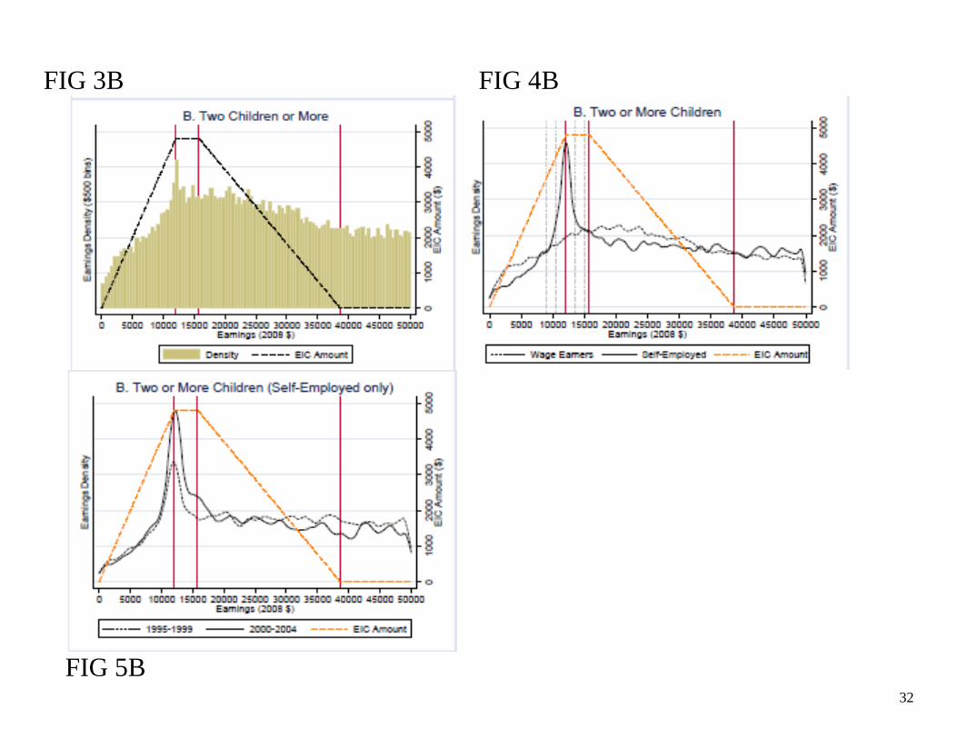
32
FIG 3B FIG 4B
FIG 5B

33
• Federal Income Tax: − More complicated to show since the schedule varies across family types
(marital status), number of children, and deductions. Normalize rel to 0. − Some evidence of bunching around 1st kink (MTR goes from 0 15%) − Figures 6/7 − More evidence for single and HH returns − First kink probably the most “visible” to taxpayer. But could the finding be
an artifact that those left of 1st kink do not have to file and may not be in data? − No evidence at 2nd or later kinks

34

35

36
Implication: -- Small elasticities for wage earners -- Simulations using extended model again shows no clustering. So these models are not right or elasticities are small or agents do not know where kinks are. -- Problematic for research using kinked budget constraint methods

37
WHY NOT MORE BUNCHING AT THE KINKS? 1) True intensive elasticity of response may be small (may partly be due to inability to adjust hours) 2) Randomness in income generation process: Saez, 2002 shows that year-to-year income variation too small to erase bunching if elasticity is large 3) Information and salience a) Liebman and Zeckhauser: “Schmeduling” (behavioral model where individuals confuse MTR with average tax rate) b) Chetty and Saez (2009): information significantly affects bunching in EITC field experiment 4) Adjustment costs and institutional constraints (Chetty et al 2009)

38
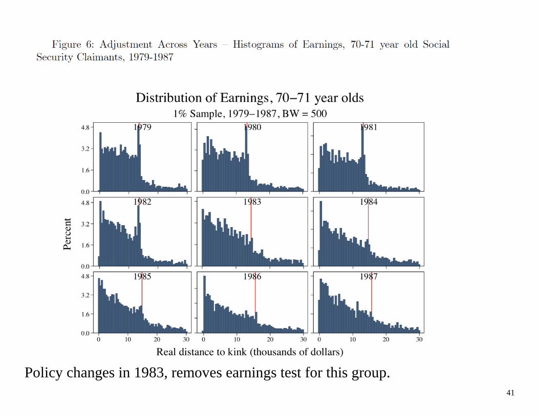
OTHER EVIDENCE ON BUNCHING 1) Social Security Earnings Test: “Barriers to Individual Earnings Adjustment to the Social Security Earnings Test” by Gelber, Jones, and Sacks What is it: once you claim social security, you can continue to have earnings. But depending on your age and your earnings amount, your SS benefit may be reduced as your earnings increase. The policy in 2012: Age 62-65, benefits reduced by 50 cents for every extra dollar earned above $14,640 Above age 65, there is no earnings test There is substantial variation in the policy over time; back in the 1990s the earnings test was applied to all workers regardless of age. They study bunching, implied elasticities AND time to adjustment. Data: 1% sample of SS earnings master file (panel data on earnings) LEHD, gives information on type of employer

39
Policy affects those age 62-69.

40
41
Policy changes in 1983, removes earnings test for this group.

42

43
Implied elasticities: 0.74 0.34 when they constrain adjustment costs to be zero.

44
Other settings where we might expect to see bunching: Medicaid Jobs First (Bitler, Gelbach and Hoynes AER 2006 looked but did not find any) Absence of bunching at nonconvex kink in TANF

45
Friedberg 2000: Social Security Earnings Test 1) Uses CPS data on labor supply of retirees receiving Social Security benefits 2) Studies bunching based on responses to Social Security earnings test
• Earnings test: phaseout of SS benefits with earnings above an exempt amount around $14K/year
• Today: Phaseout rate varies by age group: 50% (below 66), 33% (age 66), 0 (above 66)
3) Friedberg exploits a 1983 reform (change in SS earnings test) Estimates elasticities using Hausman method, finds relatively large compensated and uncompensated elasticities. Finds some evidence of bunching on kink (but data is not as good as Saez). May be that this is more salient.

46
CHETTY, FRIEDMAN, OLSEN, AND PISTAFERRI (2011) 1) If workers face adjustment costs, may not reoptimize in response to tax changes of small size and scope in short run a) Search costs, costs of acquiring information about taxes b) Institutional constraints imposed by firms (e.g. 40 hour week); that may emerge endogenously in equilibrium. 2) Could explain why “macro” studies find larger elasticities 3) Question: How much are elasticity estimates affected by frictions?

47
Chetty et al. 2011: Model 1) Firms post jobs at a set hours value (wage-hours offers , ( )j jh w h ). Firm can not change hours after matching with worker (hours constraint) 2) Workers draw from this distribution and must pay search cost to reoptimize (so they only search if potential gains exceed costs). Nest “standard” model by setting search costs to 0. 3) Therefore not all workers locate at optimal choice 4) Bunching at kink and observed responses to tax reforms attenuated 5) Individual bunching (individuals chose to locate at the kink via job search) vs aggregate bunching (aggregation of worker preferences by unions or firms; even individuals who don’t have the incentive to locate there do)

48
Chetty et al. 2011: Testable Predictions Model generates three predictions: 1) [Size] Larger tax changes generate larger observed elasticities Large tax changes are more likely to induce workers to search (potential gains more likely to exceed search costs) for a different job 2) [Scope] Tax changes that apply to a larger group of workers generate larger observed elasticities Firms tailor jobs to preferences of common workers Individual bunching (individual locate at kink through search) vs aggregate bunching (aggregation of worker’s preferences by unions or firms). 3) [Search Costs] Workers with lower search costs exhibit larger elasticities from individual bunching

49

50
Chetty et al. 2011: Data Matched employer-employee panel data with admin tax records for full population of Denmark 1994-2001 1) Income vars: wage earnings, capital and stock income, pension contributions 2) Employer vars: tenure, occupation, employer ID 3) Demographics: education, spouse ID, kids, municipality Sample restriction: Wage-earners aged 15-70, 1994-2001 Approximately 2.42 million people per year

51
Institutional Setting 1) heavily unionized labor force (most private sector workers covered by collective bargaining). Wages set at occupation/seniority level Renegotiated every 2-4 years 2) 3 bracket MTR system, 25% pay top MTR 3) tax variation: within tax-year (across brackets) and across year. Larger variation exists within tax-year. Brackets adjusted for real growth with lag.
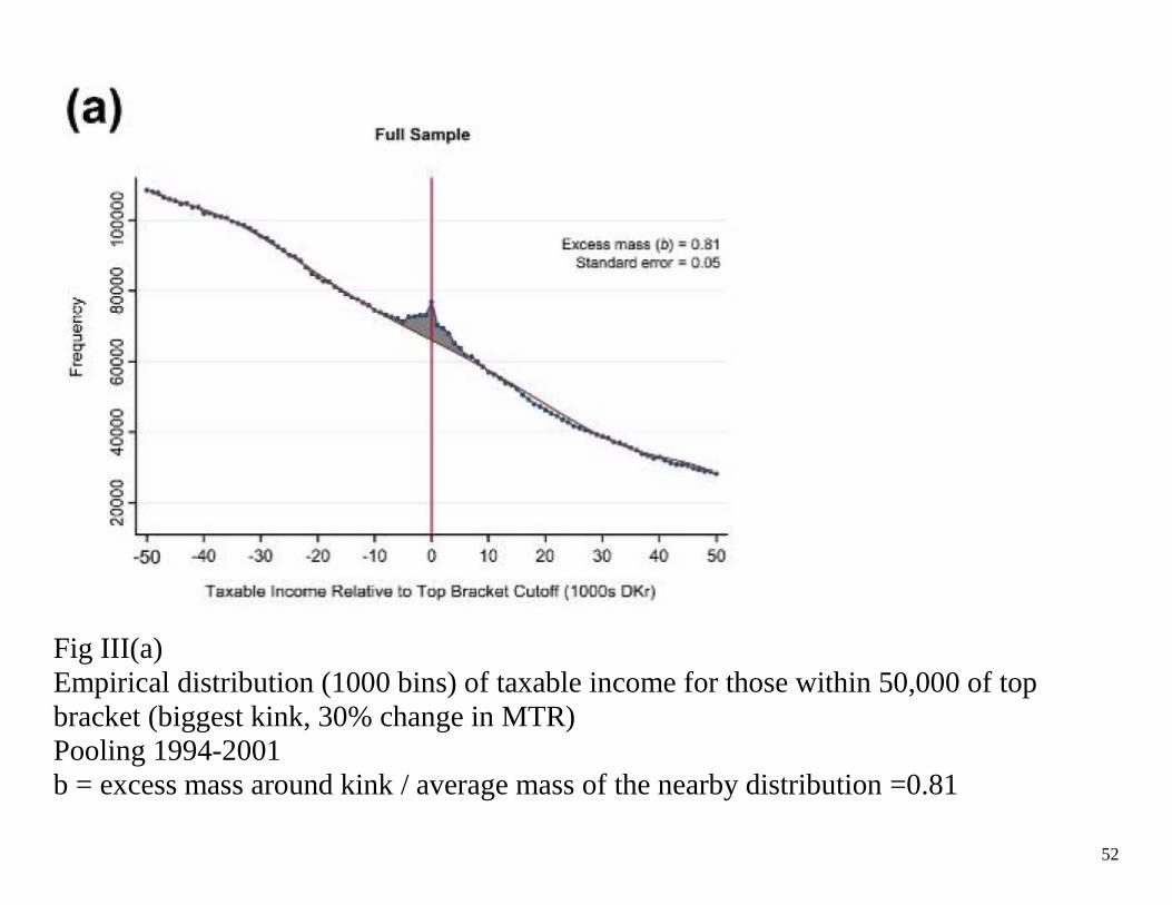
52
Fig III(a) Empirical distribution (1000 bins) of taxable income for those within 50,000 of top bracket (biggest kink, 30% change in MTR) Pooling 1994-2001 b = excess mass around kink / average mass of the nearby distribution =0.81

53
(b) larger clustering (=larger elasticities) for married women (c) larger clustering for teachers compared to military

54
Figure IV: shows that the excess mass moves as the kink increases (automatic indexing of brackets) Figure VI: Consistent with prediction that larger bunching with tax changes are larger (only present for top bracket)

55
Shows that bunching holds not only using own incentives (e.g. bottom graph) but group’s incentives. Their narrative: because of the increase in the MTR there is a discontinuous return to wages above the top kink. They instead would try to negotiate over other dimensions Bottom graph – these guys have deductions that mean that the statutory kink is not equal to their real kink. Yet there is still clustering (but less). Fig VIII – shows the “peaked” income bin by occupation and shows that they are disproportionately to the left of the kink.

56
Chetty et al. 2011: Results 1) Search costs attenuate observed behavioral responses substantially 2) Firm responses and coordination critical for understanding behavior: individual and group elasticities may differ significantly 3) Nonlinear budget set models may fit data better if these factors are incorporated 4) Standard method of estimating elasticities using “small tax reforms” on same data yields close-to-zero elasticity estimate [not sure why they do a diff-diff here rather than looking at how/if the bunching moves with reform] 5) Placebo test: Much more bunching (and at all kinks) for self employed (who presumably do not face hours constraints or adjustment costs). So the predictions should not hold for this group. 6) Illustrates aggregate bunching, that is the bunching for worker’s who do not have own incentives to locate at the kink.

57
Chetty et al 2010 Thoughts External validity:
1. Denmark less complex labor market, highly unionized. Easier to facilitiate supply-side optimizing.
2. Cross-sectional tax variation is not always larger than “small tax reforms” (see Eissa TRA86)
3. Is the tax schedule more “salient”, “observable” – 60% of wage earners have zero deductions.
How do we know that all of the adjustment is by the “agent” (e.g., union)? Does this have the same meaning as individual adjustment?

58
REDUCED FORM LABOR SUPPLY LITERATURE: RESULTS Literature exploits variation in taxes/transfers to estimate hours and participation elasticities 1) Return to simple model where we ignore non-linear budget set issues 2) Large literature in labor/public economics estimates effects of taxes and wages on hours worked and participation

59
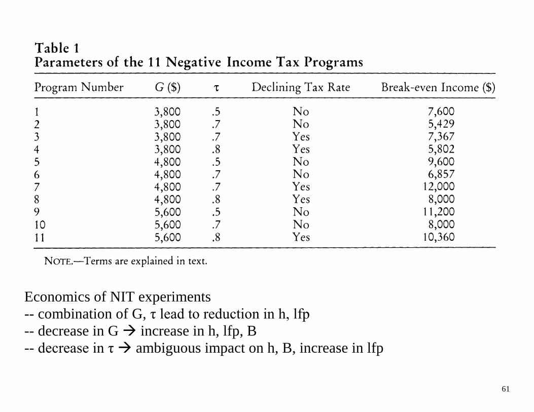
NEGATIVE INCOME TAX (NIT) EXPERIMENTS 1) Best way to resolve identification problems: exogenously increase the marginal tax rate with a randomized experiment 2) NIT experiment conducted in 1960s/70s in Denver, Seattle, and other cities 3) First major social experiment in U.S. designed to test proposed transfer policy reform 4) Provided lump-sum welfare grants G combined with a steep phaseout rate τ (50%-80%) [based on family earnings] 5) Analysis by Rees (1974), Munnell (1986) book, Ashenfelter and Plant JOLE'90, and others 6) Several groups (varying G, τ) with randomization within each; approx. N = 75 households in each group.

60
EXPERIMENTAL PRIMER Why we like them: Evaluate changes without model, functional form assumptions. Evaluate new policies (no “natural” variation) How we evaluate them: Difference in mean T – C Why no pre vs post? What do we need to check: 1) T is exogenous: balance in Xs and pre-RA y between T and C 2) no impact of T on sample over time (attrition)
61
Economics of NIT experiments -- combination of G, τ lead to reduction in h, lfp -- decrease in G increase in h, lfp, B -- decrease in τ ambiguous impact on h, B, increase in lfp
62
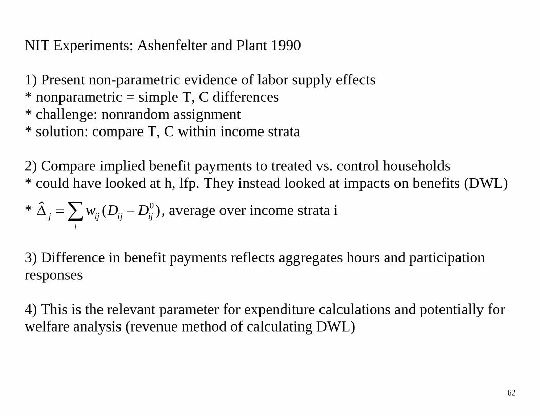
NIT Experiments: Ashenfelter and Plant 1990 1) Present non-parametric evidence of labor supply effects * nonparametric = simple T, C differences * challenge: nonrandom assignment * solution: compare T, C within income strata 2) Compare implied benefit payments to treated vs. control households * could have looked at h, lfp. They instead looked at impacts on benefits (DWL)
* 0ˆ ( )j ij ij iji
w D D∆ = −∑ , average over income strata i
3) Difference in benefit payments reflects aggregates hours and participation responses 4) This is the relevant parameter for expenditure calculations and potentially for welfare analysis (revenue method of calculating DWL)

63
5) Shortcoming: approach does not decompose estimates into income and substitution effects and intensive vs. extensive margin [they focused on “program evaluation”] 6) Hard to identify the key elasticity relevant for policy purposes and predict labor supply effect of other programs

64
Because so many T groups it is hard to see how changing G and t affect outcomes.

65
Attrition is a real problem here. Key is that they collected earnings data through survey and there is no incentive to stick with it if you expect no benefit (e.g. do not receive NIT)

66
NIT Experiments: Overall Findings 1) Significant labor supply response but small overall 2) Implied earnings elasticity for males around 0.1 3) Implied earnings elasticity for women around 0.5 4) Academic literature not careful to decompose response along intensive and extensive margin 5) Response of women is concentrated along the extensive margin (can only be seen in official govt. report) 6) Earnings of treated women who were working before the experiment did not change much
67
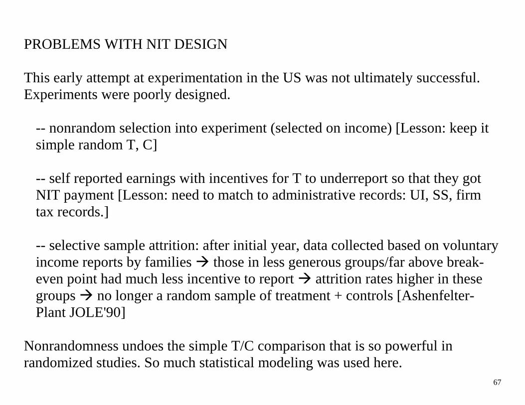
PROBLEMS WITH NIT DESIGN This early attempt at experimentation in the US was not ultimately successful. Experiments were poorly designed.
-- nonrandom selection into experiment (selected on income) [Lesson: keep it simple random T, C] -- self reported earnings with incentives for T to underreport so that they got NIT payment [Lesson: need to match to administrative records: UI, SS, firm tax records.] -- selective sample attrition: after initial year, data collected based on voluntary income reports by families those in less generous groups/far above break-even point had much less incentive to report attrition rates higher in these groups no longer a random sample of treatment + controls [Ashenfelter-Plant JOLE'90]
Nonrandomness undoes the simple T/C comparison that is so powerful in randomized studies. So much statistical modeling was used here.

68
NATURAL EXPERIMENTS True experiments are costly to implement and hence rare. However, real economic world (nature) provides variation that can be exploited to estimate behavioral responses “Natural Experiments'” Natural experiments sometimes come very close to true experiments:

69
Imbens, Rubin, Sacerdote AER '01 It is unusual to have experimentally manipulated income to identify income effects (on labor supply). This paper provides evidence from lottery winnings. -- Survey of lottery winners and nonwinners (=winners of small prize) matched to Social Security administrative data to estimate income effects. * matching to administrative data is a plus (pre trends) -- Lottery generates random assignment conditional on playing
* variation in prize amount is random
-- Find significant but relatively small income effects: lwy
δηδ
= = -0.05 to -0.10
-- Identification threat: differential response-rate among groups * 49% for nonwinners, 42% for winners

70
Mixes up evaluation of validity of design: Comparing Xs and Y pre-treatment [key is testing for differences between columns 3 & 4 in pre-period] with Unconditional treatment effects Problem: unbalanced T and C groups.

71
Good pre-trends Larger impact for larger prize winners

72
Same. Parametric model results (regress on continuous prize measure) yields estimate for income effect of -0.05 – 0.10

73
Threats and thoughts: External validity: lottery winners not random Attrition
74
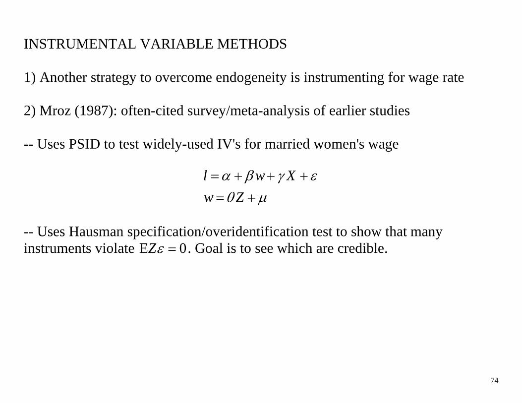
INSTRUMENTAL VARIABLE METHODS 1) Another strategy to overcome endogeneity is instrumenting for wage rate 2) Mroz (1987): often-cited survey/meta-analysis of earlier studies -- Uses PSID to test widely-used IV's for married women's wage
l w Xw Z
α β γ εθ µ
= + + += +
-- Uses Hausman specification/overidentification test to show that many instruments violate E 0Zε = . Goal is to see which are credible.

75
Hausman Test 1) Suppose you can divide instrument set into those that are credibly exogenous (Z) and those that are questionable ( *Z ) 2) Null hypothesis: both are exogenous 3) Alternative hypothesis: *Z is endogenous 4) Compute IV estimate of β with small and large instrument set and test for equality of the coefficients 5) Note that is often a very low power test (accept validity if instruments are weak)

76
MROZ RESULTS Background variables he maintains as credible [unemp rate, parent's ed, wife's age and ed] Tests show that the following variables fail the Hausman test: labor market experience, age hourly earnings, and previous reported wages Shows that earlier estimates in the literature are very nonrobust. This study contributed to emerging view that policy variation (taxes) was necessary to identify parameters.
Blundell et al, Econometrica, Use demographics, tax reform in IV setting

77
TAX REFORMS AND LABOR SUPPLY Modern studies use tax reforms as a “natural experiment” to evaluate the effect of taxes on labor supply (and other outcomes). Can get around problem of endogenous net of tax wages and wages more generally o Advantage of tax reform: policies can affect some groups and not others,
creating natural treatment and control groups. o We have seen lots of changes in tax laws to provide experiments to examine.
TRA86 Tax Reform Act of 1986 • Tons of papers on this. Why? (See Auerbach and Slemrod JEL) • Most significant policy change in postwar period • Goals of TRA86: Horiz Equity, Efficiency (eliminate tax preferences), Simplicity • Result: Broaden base + reduce rates MTR • 1986: 14 brackets, 11% - 50% • 1990: 5 brackets 0, 15, 28, 33, 28 • Increase standard deduction and personal exemptions • We will see later papers using this variation to look at impact of taxes on low
end (EITC) and high end

78
EISSA (1995): TRA86 AND MARRIED WOMEN’S LABOR SUPPLY Never published (not sure why), but great teaching paper and also very influential paper -- Established convincingly that married women are sensitive to taxes, have higher elasticity of labor supply -- Added to our knowledge that participation margin is more sensitive than hours margin -- Good example of early difference in difference methodology -- Eissa focuses on high income women because they had the highest reductions in MTR (see figure from paper)

79

80
Economics: Secondary Earner Labor supply model Most common approach is to model labor supply of husband and wife sequentially (1) Husband (or primary earner) maximizes utility ignoring wife (just like single agent model) Max(lh, Y) s.t. whhh + N = Y hh * (2) Wife (or secondary earner) maximizes utility conditioning on husband’s optimal labor supply decision
Therefore, she takes N + whhh* as given Max(lw, C) s.t. wwhw + (whhh* + N) = C
Graph this

81
Comparative statics of secondary earner model • Earnings of husband increase ↑ (through increase in h or w) nonlabor
income of wife ↑ income effect hours and employment of wife ↓. • Taxes? Decrease in taxes leads to: − ↑ net nonlabor income hours and employment of wife fall − ↑ ww hours (?), employment ↑ − KEY: with progressive taxes, she gets the change in MTR which is
exogenous to her own labor supply, but comes through her husband. Her first hour MTR is his last hour MTR.

82
Diff-in-Diff (DD) Methodology: Step 1: Simple Difference Outcome: LFP (labor force participation) Two groups: Treatment group (T) which faces a change [women married to high income husbands] and control group (C) which does not [women married to middle income husband] Simple Difference estimate: T CLFP LFP∆ = − captures treatment effect if absent the treatment, LFP equal across 2 groups Note: Rarely holds in nonexperimental setting (always holds when T and C status is randomly assigned) What to test for: Compare LFP before treatment happened (period 0)
0 0 0T CLFP LFP∆ = −

83
Step 2: Diff-in-Difference (DD) If 0 0∆ ≠ , we can estimate the DD: 1 1 0 0( ) ( )T C T CLFP LFP LFP LFP∆∆ = − − − (0 = after reform, 1 = before reform) DD is unbiased if parallel trend assumption holds: Absent the change, difference across T and C would have stayed the same before and after. Regression estimation of Unconditional DD:
0 1
1 1 0 0
*
ˆ ( ) ( )it
T C T C
LFP AFTER TREAT AFTER TREAT
LFP LFP LFP LFP
α β β γ ε
γ
= + + + +
= − − −

84
Diff-in-Diff (DD) Methodology DD most convincing when groups are very similar to start with [closer to randomized experiment] motivation for RD Can test DD using data from more periods and plot the two time series to check parallel trend assumption Use alternative control groups [not as convincing as potential control groups are many] In principle, can create a DDD as the difference between actual DD and placeboDD (DD between 2 control groups). However, DDD of limited interest in practice because (a) if 0placeboDD ≠ , DD test fails, hard to believe DDD removes bias (b) if 0placeboDD = , then DD=DDD but DDD has higher s.e.
85
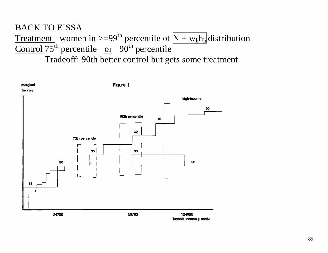
BACK TO EISSA Treatment women in >=99th percentile of N + whhh distribution Control 75th percentile or 90th percentile
Tradeoff: 90th better control but gets some treatment

86
Data CPS 1984 – 1986 before (83 – 85) 1990 – 1992 after (89 – 91) TRA86 phased in by 88 Predictions? -- Employment of women in 99th p will rise relative to women in 90th p Her MTR ↓ net wage ↑ LFP ↑ -- But we have to believe that her net of tax nonlabor income did not change much. Why? husband’s MTR ↓ ( ↑ earnings) (or no change if elas small)
But TRA86 broadened base overall effect on her after tax non-labor income is small * To the extent which his ↓ net earnings are not captured, then, this estimate is an underestimate of total effect.

87
Results Unconditional difference in difference Ave Y ∆MTR(Tab IIa) ∆LFP (Tab III) D in D 99th p > 90K -13.9 pp +9.0 pp 90th p 67K -6.9 pp +4.5 pp +4.5 pp. (2.8) 13% 75th p 47K -4.1 pp +5.3 pp +3.7 pp (2.8) 12% Ave Y ∆MTR(Tab IIa) ∆hours (Tab III D in D 99th p > 90K -13.9 pp +163 90th p 67K -6.9 pp +96 +67 (64.8) 6% 75th p 47K -4.1 pp +55 +108 (65.1) 9%

88
Conditional D-D 0 1 2 3 4Pr( ) 86 ( * 86)it i t i itWork Z high Post High Postα α α α α= + + + +
Zit = age, educ, # kids, young kids, race, CC, year & state fixed effects Expectations α2< 0 baseline inc. effect α3> 0 secular trend α4> 0 Main test of TRA86 Results -- Large response for participation, less for hours -- Consistent w/ lit showing greater responsiveness on participation margin than hours margin (Mroz, Hausman)

89

90
Caveats of Eissa Results • Does “common trends” assumption hold?
o Possible story: Assortative mating on unobservables. Trend toward "power couples." Used to be that prof men had nonworking spouses; now more common to have working prof spouse. Yet in middle class more stable situation with working middle class spouse.
o Demand or supply shock to 99th p (e.g. work in different sectors) different trends for T and C reflecting inequality literature
• LFP is very different between T and C (never a good thing) • Things to examine in DD model that were not known then:
o Placebo treatment (use data for pre periods, redo DD using placebo treatment, say comparing year 0 and year -1)
o Useful (necessary) to plot outcome variables in T and C year on year for whole period; examine whether the trends are similar in pre period. Look for change.
o Liebman and Saez (2006) plot full time-series CPS plot and show that Eissa's results are not robust using admin data (SSA matched to SIPP) [unfortunately, IRS public tax data does not break down earnings within couples] See next page.

91

92
Econometrics of Kinked Budget Constraints: Convex Budget Set (Hausman’s model)
Preferences: h* = h ( w , y , ε ) (functional form for labor supply equation) h = observed hours ε = taste shifter
h
h0 = 0
y3
y5
h6 h4
h2
-w5 -w3
-w1 y1
After tax and transfer income

93
Comments: -Virtual income y3, y5 are a function of observed non-labor income and tax system. -Need one preference assumption (either labor supply equation, IUF or DUF) -Assume gross wage is exogenous -Assume gross nonlabor income is exogenous Ex: Functional form Hausman used for labor supply equation was
εγβα +++= zyiwihi* which implied the following for the IUF:
]2^
)[exp(),(βγ
βα
βαβ zwiyiwiyiwiv +−+=

94
4 Steps in constructing the likelihood function:
1. What do you observe? 2. Identify possible states 3. Determine economic decision rule that justifies each choice 4. Derive probabilities associated with each choice
(Step 1) What do you observe? Hours (0, or continuous hours worked) Hourly wage rate, for workers Nonlabor income Covariates (Step 2) States of the World 0 h = 0 1 0 < h < h2 2 h = h2 3 h2 < h < h4 4 h = h4 5 h4 < h < h6 6 h= h6

95
Define the labor supply function for each segment: h(wi,yi,ε) linear labor supply curve for net wage wi, and net nonlabor income yi i=1,2,3 Ex: w1=w (no taxes) w3=w(1-t1) 1st marginal tax rate w5=w(1-t2) 2nd marginal tax rate y1=N observed nonlabor income y3 virtual income y3 y5 virtual income y5

96
(Step 3) Economic Decision Rules State 0 h = 0
h( w1 , y1 , ε ) ≤ 0 Desired hours given w1, y1 are <0
State 1 0 < h < h2 h = h( w1 , y1 , ε ) Desired hours given w1,y1 are between 0 and h2 State 2 h = h2
h( w1 , y1 , ε ) ≥ h2 AND h( w3 , y3 , ε ) ≤ h2 Note that being on kink has higher probability than any given point on segment.
State 3 h2 < h < h4 h = h( w3 , y3 , ε )
State 4 h = h4
h( w3 , y3 , ε ) ≥ h4 AND h( w5 , y5 , ε ) ≤ h4 State 5 h4 < h < h6
h = h( w5 , y5 , ε ) State 6 h = h6
h( w5 , y5 , ε ) ≥ h6

97
Then translate desired hours rule into rule about unobservable ( ε ) Derive probability that choice was made (Step 4) Create Likelihood Function L ( h ) = П [ Pr ( δi = 0 ) ] ^ ( δi ) П [ f ( h | wi , yi ) ] ^ ( δi ) where δi = 1 if state i is observed, and = 0 otherwise.
i = 0,2,4,6 i = 1,3,5


