Hillsborough County SWMM4.31B User’s Manual · The Storm Water Management Model (SWMM) was...

1

Hillsborough County SWMM4.31B

User’s Manual

Stormwater Management SectionPublic Works Department

Hillsborough County

Tampa, Forida

March, 2000

2

Content

List of Tables

List of Figures

1. Introduction ………………………………………………………………………….4

2. Runoff Calculation ………………………………………………………………… .6

2.1 SCS-CN Method2.2 SCS Dimensionless Hydrograph2.3 Model Implementation2.4 Discussion on Hydrograph Shape Factor, K2.5 Input Format

3. Modifications of Extran Block ……………………………………………………..26

3.1 Minor Losses3.2 Pipe Extension3.3 Pipe Shape3.4 Input Format

4. Modifications of Combine Block ………………………………………………….30

5. Input of EXTRAN and COMBINE Blocks ………………………………………..31

Appendix A Overland Flow Manning’s n

Appendix B Minor Loss Coefficient

3

List of Tables

Table 2.1a Runoff Curve Numbers for Urban Areas ……………………………….5

Table 2.1b Runoff Curve Numbers for Cultivated Agricultural Lands …………….7

Table 2.1c Runoff Curve Numbers for Other Agriculture Lands …………………9

Table 2.1d Runoff Curve Numbers for Arid and Semiarid Rangeland …………..11

Table 3.1 Pipe Type Classification ……………………………………………….24

Table 3.2 Changes of Input Format ………………………………………………25

Table 4.1 List of A1 Card Options ………………………………………………26

List of Figures

Figure 2.1 Definition of Unit Hydrograph …………………………………………… 13

4

1. Introduction

The Storm Water Management Model (SWMM) was developed for the Environmental

Protection Agency in 1969-1971 as a single-event model for simulation of quantity

processes in combined sewer systems (Metcalf and Eddy et al., 1971). It has since been

applied to virtually every aspect of urban drainage, from routine drainage design to

sophisticated hydraulic analysis to non-point source runoff quality studies, using both single

event and continuous simulation. Through subdividing large catchments and flow routing

down the drainage system, SWMM can be applied to catchments of almost any size, from

parking lots to subdivisions to cities.

The current version of SWMM4.31 is segmented into several computational “Blocks”:

• The Runoff block generates runoff from rainfall using a nonlinear reservoir

method and does simple flow routing by the same method. Subsurface flow routing of

water infiltrated through the soil surface is optional.

• The Thansport block performs flow routing using a kinematic wave technique.

• The Extran block performs flow routing by an explicit finite-difference solution of the

complete St. Venant equations.

• The Storage/Treatment block routes through storage units using the Puls (storage

indication) method.

• The Statistics block separates continuous simulation hydrographs and pollutographs

(concentration vs. time) into independent storm events, calculates statistical moments, and

performs elementary frequency analyses.

Water quality may also be simulated in all blocks except Extran, and the output from

continuous simulation may be analyzed by the statistics block.

5

Hillsborough County of Florida has been using SWMM model for many years. Mostly only

Runoff and Extran blocks were used. While using this model, the storm water modeling

group of Hillsborough County made many modifications based on the watershed conditions

of the county. All the modifications will be summarized in the following sections.

6

2. Runoff Calculation

In the Hillsborough County version of SWMM model, the SCS-CN method, rather than the

nonlinear reservoir method, was used to calculate the runoff discharge used in Extran

Block.

2.1 SCS-CN method

The Soil Conservation Service-curve number (SCS-CN) method is one of the most popular

methods for computing the volume of surface runoff for a given rainfall event from small

watersheds. Kent (1973) described and examined this method in detail. The SCS-CN

method is based on the water balance equation and two fundamental hypotheses. The first

hypothesis states that the ratio of the actual amount of direct runoff to the maximum

potential runoff is equal to the ratio of the amount of actual infiltration to the amount of the

potential maximum retention. The second hypothesis states that the amount of initial

abstraction is some fraction of the potential maximum retention. Expressed mathematically,

the water balance equation and the two hypotheses, respectively, are

Ea PFIP ++= (2-1)

SF

IP

P

a

E =−

(2-2)

SI a λ= (2-3)

where P = total precipitation, inch;

Ia = initial abstraction, inch;

7

F = cumulative infiltration excluding Ia, inch;

λ= non-dimensional parameter;

PE = direct runoff, inch; and

S = potential maximum retention or infiltration, inch

The current version of the SCS-CN method assumes λequal to 0.2 for usual practical

application. As the initial abstraction component accounts for surface storage, interception,

and infiltration before runoff begins, λ can take any value ranging from 0 to 1. Combining

(2-1) and (2-2), we can write an equation for PE as follows:

SIP

IPP

a

aE +−

−=

2)( (2-4)

If λ=0.2, then

SP

SPPE 8.0

)2.0( 2

+−= (2-5)

By studying the relationships of many different watersheds, the SCS further

introduced a dimensionless number, CN, called curve number. The curve number

and S are related by

101000 −=CN

S (2-6)

The curve number is a function of land use, cover, soil classification, hydrologic conditions,

and antecedent runoff conditions. The variation in infiltration rates of different soils is

incorporated in curve number selection through the classification of soils into four hydrologic

soil groups: A, B, C, and D. These groups, representing soils having high, moderate, low, and

very low infiltration rates, are as follows:

8

Group A: soils have low runoff potential and high infiltration rates even when thoroughly

wetted. They consist chiefly of deep, well to excessively drained sands or gravels and have a

high rate of water transmission (greater than 0.30 in/h).

Group B: soils have moderate infiltration rates when thoroughly wetted and consist chiefly

of moderately deep to deep, moderately well drained to well drained soils with moderately

fine to moderately coarse texurse. These soils have a moderate rate of water transmission

(0.15-0.30 in/h).

Group C: soils have low infiltration rates when thoroughly wetted and consist mainly of soils

with a layer that impedes downward movement of water and soils with moderately fine to

fine texture. These soils have a low rate of water transmission (0.05-0.15 in/h).

Group D: soils have high runoff potential. They have very low infiltration rates when

thoroughly wetted and consist chiefly of clay soils with a high swelling potential, soils with a

permanent high water shallow soils over nearly impervious material . These soils have a very

low rate of water transmission (0-0.05 in/h)

Runoff curve numbers for urban areas, cultivated and other agricultural lands, and arid and

semiarid rangelands are shown in Table 2.1

Table 2.1a Runoff Curve Numbers for Urban Areas*

9

Curve numbers for

hydrologic soil groupCover type and hydrologic condition

Average

percentage of

impervious

area**A B C D

Fully developed urban areas (vegetation established)

Open space (lawns, parks, golf courses, cemeteries,

etc.)***

Poor condition (grass cover < 50%) 68 79 86 89

Fair condition (grass cover 50% to 75%) 49 69 79 84

Good condition (grass cover > 75%) 39 61 74 80

Impervious areas:

Paved parking lots, roofs, driveways, etc. (excluding

Right-of-way)

98 98 98 98

Streets and roads:

Paved; curbs and storm sewers (excluding right-of-

way)

98 98 98 98

Paved; open ditches (including right-of-way) 83 89 92 93

Gravel (including right-of-way) 76 85 89 91

Dirt (including right-of-way) 72 82 87 89

Western desert urban areas:

Natural desert landscaping (pervious areas only) 63 77 85 88

Artificial desert landscaping (impervious weed barrier,

desert shrub with 1- to 2-inch sand or gravel mulch,

and basin borders

96 96 96 96

Urban districts:

Commercial and business 85 89 92 94 95

Industrial 72 81 88 91 93

Residential districts by average lot size:

1/8 acre or less (town house) 65 77 85 90 92

¼ acre 38 61 75 83 87

10

1/3 acre 30 57 72 81 86

½ acre 25 54 70 80 85

1 acre 20 51 68 79 84

2 acre 12 46 65 77 82

Developing urban areas:

Newly graded areas (pervious areas only, no

Vegetation)

77 86 91 94

Idle lands (CNs are determined through the use of

cover types similar to those for other agricultural

lands.)

* Average runoff condition, and Ia = 0.2S.

** The average percentage of impervious area shown was used to develop the composite CNs. Other assumptions are

as follows: Impervious areas are directly connected to the drainage system; impervious areas have a CN of 98; and

pervious areas are considered equivalent to open space in good hydrologic condition.

*** CNs shown are equivalent to those of pasture. Composite CNs may be computed for other combinations of open

space cover type.

Table 2.1b Runoff Curve Numbers for Cultivated Agricultural Lands *

11

Curve numbers for

hydrologic soil groupCover type Treatment** Hydrologic

Condition***

A B C D

Bare soil 77 86 91 94

Poor 76 85 90 93FallowCrop residue cover (CR)

Good 74 83 88 90

Poor 72 81 88 91Straight row (SR)

Good 67 78 85 89

Poor 71 80 87 90SR+CR

Good 64 75 82 85

Poor 70 79 84 88Contoured (C)

Good 64 74 81 85

Poor 69 78 83 87C+CR

Good 64 74 81 85

Poor 66 74 80 82Contoured and terraced

(C&T) Good 62 71 78 81

Poor 65 73 79 81

Row crops

C&T+CRGood 61 70 77 80

Poor 65 76 84 88SR

Good 63 75 83 87

Poor 64 75 83 86SR+CR

Good 60 72 80 84

Poor 63 74 82 85C

Good 61 73 81 84

Poor 62 73 81 84C+CR

Good 60 72 80 83

Poor 61 72 79 82C&T

Good 59 70 78 81

Small grain

C&T+CR Poor 60 71 78 81

Good 58 69 77 80

12

Poor 66 77 85 89SR

Good 58 72 81 85

Poor 64 75 83 85C

Good 55 69 78 83

Poor 63 73 80 83

Close-seeded

or broadcast

legumes or

rotation

meadow C&TGood 51 67 76 80

* Average runoff condition, and Ia = 0.2S.

** Crop residue cover applies only if residue is on at least 5% of the surface throughout

the year.

*** Hydrologic condition is based on a combination of factors that affect infiltration and

runoff, including (a) density and canopy of vegetative areas, (b) amount of year-round

cover, (c) amount of grass or close-seeded legumes in rotations, (d) percentage of residue

cover on the land surface (good > 20%), and (e) degree of surface roughness.

Poor: Factors impair infiltration and tend to increase runoff.

Good: Factors encourage average and better-than-average infiltration and tend to

decrease runoff.

13

Table 2.1c Runoff Curve Numbers for Other Agriculture Lands 1

Curve numbers for

hydrologic soil groupCover typeHydrologic

conditionA B C D

Poor 68 79 86 89

Fair 49 69 79 84

Pasture, grassland, or range-continuous forage

for grazing2

Good 39 61 74 80

Meadow-continuous grass, protected from

grazing and generally mowed for hay30 58 71 78

Poor 48 67 77 83

Fair 35 56 70 77Brush—brush-weed-grass mixture with brush the

major element3

Good 304 48 65 73

Poor 57 73 82 86

Fair 43 65 76 82Woods—grass combination (orchard or tree

farm)5

Good 32 58 72 79

Poor 45 66 77 83

Fair 36 60 73 79Woods6

Good 304 55 70 77

Farmsteads—buildings, lanes, driveways, and

surrounding lots59 74 82 86

14

1 Average runoff condition, and Ia = 0.2S.2 Poor: <50% ground cover or heavily grazed with no mulch.

Fair: 50% to 75% ground cover and not heavily grazed.

Good: >75% ground cover and lightly or only occasionally grazed.3 Poor: <50% ground cover.

Fair: 50% to 75% ground cover.

Good: > 75% ground cover.4 Actual curve number is less than 30; use CN=30 for runoff computations.5CNs shown were computed for areas with 50% woods and 50% grass(pasture) cover.

Other combinations of conditions may be computed from the CNs for woods and pasture.6Poor: Forest litter, small trees, and brush are destroyed by heavy grazing or regular

burning.

Fair: Woods are grazed but not burned, and some forest litter covers the soil.

Good: Woods are protected from grazing, and litter and brush adequately cover the soil.

15

Table 2.1d Runoff Curve Numbers for Arid and Semiarid Rangeland*

Curve numbers for

hydrologic soil groupCover TypeHydrologic

condition**

A*** B C D

Poor 80 87 93

Fair 71 81 89

Herbaceous—mixture of grass, weeds, and low-

growing brush, with brush the minor element

Good 62 74 85

Poor 66 74 79

Fair 48 57 63

Oak-aspen—mountain brush mixture of oak

brush, aspen, mountain mahogany, bitter brush,

maple, and other brush. Good 30 41 48

Poor 75 85 89

Fair 58 73 80

Pinyon-juniper—pinyon, juniper, or both; grass

understory.

Good 41 61 71

Poor 67 80 85

Fair 51 63 70

Sagebrush with grass understory.

Good 35 47 55

Poor 63 77 85 88

Fair 55 72 81 86

Desert shrub—major plants include saltbush,

greasewood, creosote bush, blackbrush, bursage,

paloverde, mesquite, and cactus. Good 49 68 79 84*Average runoff condition, and Ia = 0.2S. For range in humid regions, use the table for

other agriculture lands.** Poor: <30% ground cover (litter, grass, and brush overstory.

Fair: 30% to 70% ground cover.

Good: > 70% ground cover.*** Curve numbers for group A have been developed for desert shrub only.

16

2.2 SCS Dimensionless Hydrograph

The SCS dimensionless hydrograph is a synthetic unit hydrograph in which the discharge is

expressed by the ratio of discharge Q to peak discharge Qp and the time by the ratio of time

t to the time of rise of the unit hydrograph, Tp. The unit peak discharge is calculated by

pp T

KAU = (2-7)

where Up = unit peak discharge, cfs/inch;

A = drainage are, mile2 ;

K = hydrograph shape factor, ranging from 300 for flat swampy areas to 600

in steep terrain. SCS standard K value = 484.

Tp = time to peak, in hours.

pr

p tt

T +=2

(2-8)

where tr = storm duration, hours;

tp = drainage area lag, hours.

cp Tt 6.0= (2-9)

where Tc = time of concentration, hours.

17

Figure 2.1 shows the definition of Up, Tp, for a triangular unit hydrograph used in

Hillsborough County version of SWMM model.

Figure 2.1 Definition of Unit Hydrograph

The peak discharge for a given rainfall is calculated by

Epp PUQ = (2-10)

where Q p= peak discharge, cfs. PE is calculated with Eq. (2-5).

2.3 Model implementation

The convolution method is used to yield the direct runoff hydrograph. The convolution

equation is

D i r e c t R u n o f f

E x c e s s R a in fa l l

t r

2t p

Up

t rTp Tp1 . 6 7

18

∑≤

=+−=

Mn

mmnEmn UPQ

11 (2-11)

where PEm = excess rainfall of mth pulse, inch;

Un-m+1 = unit direct runoff at time n∆t of mth rainfall pulse, interpolated from

Fig. 2.1, cfs/inch;

∆t = time step, minutes;

Qn = total runoff at time n∆t, cfs;

M = total pulses of excess rainfall.

Following are detail procedures to calculate the direct runoff at each time step: One thing

needs to be pointed out is that, compared with original SWMM model, a new input file was

introduced. The extension of this file is .WPX. This file contains all the information of

rainfall and each sub-basin’s area, CN number, Tc , Ia , and K. The detail of this file will be

discussed in Appendix B.

1) Read rainfall information from file *.WPX ;

2) Read sub-basin information, i.e. base ID, area (in acres), Tc (in minutes.), CN number,

Ia , and K, from file *.WPX ;

3) convert Tc into hour, i.e., Tc = Tc /60 (the model input is in minutes for convenience);

4) Determine time step ∆t = 0.24Tc; If ∆t>0.5, ∆t = 0.11Tc;

5) Determine excess rainfall based on Eq. (2-5), and interpolated to ∆t time series ;

6) Calculate the direct runoffs Q(t) at each time step based on Eq. (2-11);

7) Double check model accuracy with

ESCS

ESCS

PA

dttQP |

)(|

100

∫−•=ε (2-12)

where

SP

SPP

total

totalESCS 8.0

)2.0( 2

+−

= (2-13)

8) Interpolate Q(t) to SWMM model time step Qyn(t) ;

19

9) Write out Qyn(t) to a interface file (if required).

2.4 Discussion on hydrograph shape factor, K

Theoretically speaking, the hydrograph shape factor, K, only affects the peak runoff, and

should not affect the total runoff volume. In other words, no matter what the shape factor

we use, the total runoff volume should be the same – mass conservative. However, based on

the conventional way, this mass conservative can not guarantee. Refer to Fig. 2.1, the

conventional way is,

p

Ep T

KAPQ = (2-13),

and

pppb TTTT 67.267.1 =+= (2-14)

where Tb = base time;

QP = peak runoff due to excess rainfall PE.

The direct runoff at each time step can be calculated by

≤<−

≤=

bp

p

pp

p

P

p

TtTT

tTQ

TttT

Q

tQ

67.1

67.2)( (2-15)

The total direct runoff volume is

E

T

t KAPdttQVb

335.1)(0

== ∫ (2-16)

20

That means Vt is changed with K, mass are not conservative.

To avoid this, a parameter, R, was introduced.

0.167.2 0 −=K

KR (2-17)

where K0 = standard shape factor. Here use SCS standard value of 483.4.

Redefine Tb as

pb TRT )1( += (2-18)

Then the direct runoff is

≤<−−

≤=

bp

pb

bp

pP

p

TtTTT

tTQ

TttT

Q

tQ )( (2-19)

The total volume of direct runoff is

E

E

bp

T

t

AP

APK

TQdttQVb

14.646

2/67.2

2/)(

0

0

==

== ∫ (2-20)

That means the total direct runoff volume has nothing to do with the shape factor. The shape

factor only affects the peak runoff. Mass is conservative. If K=K0, Eq. (2-16) is identical to

Eq. (2-20).

21

2.5 Input Format

The input format is identical to that of EXTRAN. That is, the first two columns are groupidentifier, and 3 to 232 columns are data line (See SWMM User’s Manual and EXTRANUser’s Manual).

Variable Description Default

ID Group Identifier None

ALPHA Description of computer run (2 lines maximum of 80 Blank

Columns per line).

IT Group Identifier None

NMIN Increment for runoff hydrograph storage 0.0 minutes

DATE Rainfall date Blank

ITIME Rainfall start time Blank

NQ Number of sub-basins Blank

(note, DATE, ITIME, and NQ are not used in the model yet, and can be blank.)

IO Group Identifier None

IPRT Print controller (see description below) 0

IPLT Plot controller (see description below) 0

22

IPRT =

0,1,2 All 3 Input Data and Intermediate and Master Summaries 4 Input Data and Master Summary 5 Job specification and Master Summary Only

IPLT =

0,1 No Printer Plots--Can be overriden on KO record2 Plot All

(note, the IPRT and IPLT functions are not implemented yet.)

JR Group Identifier None

PRCARD Card Name PREC

PTOTAL Total Rainfall (inch) 0.0

(note, PRCARD is not used in the model yet.)

PG Group Identifier None

GAGEN Rainfall Gage name Blank

PRAIN Total Rainfall at this gage (inch) 0.0

(note, 1. PRAIN is not used in the model; 2. Total gages should be less than 11.)

IN Group Identifier None

DTRAINX Time step of rainfall at this gage, minutes. 0.0

RDATE Rainfall date None

DUMMY Dummy parameter 0

(note, DUMMY is not used in the model.)

PC Group Identifier None

23

RAIN(i,1) The first rainfall distribution value None

RAIN(i,2) The second rainfall distribution value None...(Input the unit hydrograph for this gage. 10 numbers each line. Every new line should beginwith PC identifier. See the following example.)

PR Group Identifier NoneGAGEN Gage name to be used in this run. None

(note, GAGEN should be identical to one of the names in PG cards.)

WP Group Identifier None

IBASIN Sub-basin ID, integer None

JCTID Junction ID in the sub-basin None

TCMIN Time of concentration, minutes 0.0

ACRES Areas of the sub-basin, acres 0.0

CN CN curve number of the sub-basin 0

CIA Initial abstraction of the sub-basin 0.2

(note, this value has been fixed in the model. Don’t try to change it.)

K Shape factor of the sub-basin 0.0

IWPPRT Print control parameter 0

(note, IWPPRT is not used in model.)

Following is a example.

24

* ============================================================================* EAST LAKE AREA* Rainfall Distributions* JULY 13-19 1990 STORM EVENT* ============================================================================*THE FOLLOWING WPX HAS BEEN UPDATED WITH NEW CN's 3/19/99 - JG*===============================================================================ID East Lake AreaID Hillsborough County BOCC--Dept of Public Works*** This is a standard HEC-1 file. RDHEC copies the ID, *, IT, IO, JR,* PG, IN, PC, and PR records from this file. It ignores other records.**FREE*DIAGRAM* NMIN DATE ITIME NQIT 10 21JAN98 0 601**NOLIST* IPRT IPLT* 0,1,2 All* 3 Input Data and Intermediate and Master Summaries* 4 Input Data and Master Summary* 5 Job specification and Master Summary Only** 0,1 No Printer Plots--Can be overriden on KO record* 2 Plot All*IO 3 0** MULTIRATION ANALYSIS--DO NOT USE* Use Only one ratio per run for SWMM.* #####################################################* TIA RF JULY 13-19 1990 STORM EVENTJR PREC 8.0* #####################################################* #####################################################* SCS 24-HR, TYPE II FLORIDA MODIFIED DISTRIBUTION (30 MIN INCREMENTS)PGFLMOD 1.0* SCS 24-HR, TYPE II FLORIDA MODIFIED DISTRIBUTION (30 MIN INCREMENTS)IN 30 14JAN98 0PC .000 .006 .012 .019 .025 .032 .039 .047 .054 .062PC .071 .080 .089 .099 .110 .122 .134 .148 .164 .181PC .201 .226 .258 .308 .607 .719 .757 .785 .807 .826PC .842 .857 .870 .882 .893 .904 .913 .923 .931 .940PC .948 .955 .962 .969 .976 .983 .989 .995 1.00 1.00*PGEL790IN 60 13JUL90 0*This is Accumulative Rain fall for July 13-19 1990 Storm event (60min Increment)PC 0.000 0.000 0.000 0.000 0.000 0.000 0.000 0.000 0.000 0.000

25

PC 0.002 0.002 0.048 0.053 0.053 0.053 0.053 0.053 0.053 0.053PC 0.053 0.053 0.053 0.053 0.096 0.096 0.096 0.096 0.096 0.096PC 0.096 0.248 0.254 0.257 0.257 0.265 0.520 0.649 0.664 0.684PC 0.693 0.693 0.693 0.693 0.693 0.693 0.693 0.693 0.693 0.693PC 0.693 0.693 0.693 0.693 0.693 0.693 0.693 0.693 0.693 0.693PC 0.693 0.695 0.708 0.713 0.713 0.713 0.713 0.713 0.713 0.713PC 0.713 0.713 0.713 0.713 0.713 0.713 0.713 0.713 0.713 0.713PC 0.713 0.713 0.713 0.713 0.713 0.713 0.713 0.713 0.713 0.713PC 0.713 0.713 0.713 0.713 0.713 0.713 0.713 0.713 0.713 0.713PC 0.713 0.713 0.713 0.713 0.713 0.713 0.713 0.713 0.713 0.713PC 0.713 0.713 0.811 0.822 0.822 0.822 0.822 0.822 0.822 0.822PC 0.822 0.822 0.822 0.822 0.822 0.822 0.822 0.822 0.822 0.822PC 0.822 0.822 0.822 0.822 0.822 0.993 0.998 1.000 1.000 1.000* ===========================================================================* THE FOLLOWING RECORD (PR) DETERMINES WHICH OF THE ABOVE DISTRIBUTIONS* WILL BE USED FOR THE CURRENT RUN.*PREL790* ===========================================================================ZZ* NODE# BASIN OLD* NUMBER 25AREA CN Ia FC KIWP 100999 100999 62 17.8 73 0.2 256 0WP 104007 104007 24 11.7 64 0.2 256 0WP 104020 104020 22 25.2 74 0.2 256 0WP 104023 104023 15 17.6 76 0.2 256 0WP 104025 104025 15 4 76 0.2 256 0WP 104030 104030 15 3 76 0.2 256 0WP 104045 104045 15 29 78 0.2 256 0WP 104050 104050 15 9.6 77 0.2 256 0WP 104060 104060 15 6.9 82 0.2 256 0WP 104063 104063 15 2.1 65 0.2 256 0WP 104075 104075 30 34 64 0.2 256 0WP 104080 104080 15 11.8 87 0.2 256 0WP 104085 104085 24 15.6 90 0.2 256 0WP 104090 104090 15 10.6 81 0.2 256 0WP 104095 104095 15 3.4 91 0.2 256 0WP 104100 104100 15 9.5 85 0.2 256 0WP 104130 104130 34 17.5 74 0.2 256 0WP 104145 104145 21 14.9 71 0.2 256 0WP 104165 104165 33 12.4 73 0.2 256 0WP 104205 104205 19 15.4 83 0.2 256 0WP 104208 104208 15 4.9 83 0.2 256 0WP 104215 104215 15 3.1 85 0.2 256 0WP 104400 104400 15 12.9 73 0.2 256 0WP 104407 104407 38 9 65 0.2 256 0WP 104416 104416 34 8.1 70 0.2 256 0WP 104424 104424 15 4.1 93 0.2 256 0WP 104428 104428 22 11.8 78 0.2 256 0WP 104432 104432 15 10.3 91 0.2 256 0

26

3. Modifications of Extran Block

Several minor modifications have been carried out in Extran Block. These minor modifications

are: minor losses, pipe extension, pipe shape, and input format.

3.1 Minor Losses

Minor head losses have been included in the model (subroutine HEADLOSS). In B0 card,

another input flag, KMFLAG, was added (the third one). If KMFLAG = 1, the minor losses

will automatically taken into account. In this case, three minor loss coefficients, Kentrance, Kextent,

and Kothers, for each pipe are required (C1 card). If KMFLAG=0, minor losses are not

calculated.

Assume the minor losses are uniformly distributed along the pipe, based on Chezy’s Law, the

minor losses can be converted into an equivalent Manning’s coefficient, which is

gLRC

Knn t 2

3/42201 += (3-1)

where n0 = the natural Manning’s of the pipe;

Kt = Kentrance+ Kextent, + Kothers, total minor loss coefficient;

R = hydraulic radius;

g = gravity;

L = pipe length;

C = Unit conversion factor, = 1 for metric system, and = 1.486 for US custom system;

n1 = equivalent Manning’s coefficient including minor losses.

27

3.2 Pipe extension (subroutine STRETCH)

In order to avoid the stability problem, an equivalent longer pipe can be developed for an

extremely short pipe. Assuming that the equivalent pipe will have the same discharge, same

area, and same hydraulic radius, based on Checy’s Law, an equivalent Manning’s

coefficient for the longer pipe can be derived as

ee L

Lnn 0

0= (3-2)

where n0 = natural Manning’s coefficient of the pipe;

L0 = initial pipe length;

Le = extended pipe length;

ne = equivalent Manning’s coefficient.

The KMFLAG was also applied to pipe extension. That is, if KMFLAG =1, pipe extension

will automatically considered in the model. In this case, a parameter, SFACTOR, is required

in the C1 card. SFACTOR = Le/L0.

3.3 Pipe shape

In this version, the pipe types are classified as

28

Table 3.1 Pipe Type Classification

Type Pipe Shape Comments

1 Circle

2 Rectangle

3 Elliptical Horizontal. The lookup

tables for hydraulic radius

and cross-section area are

derived analytically.

4 Arch

5 Basket Handler

6 Trapezoidal

7 Parabolic

8 Natural Channel

9

3.4 Input format

All the original input formats for vertical distances, for example, ZP(1) (distance of conduit

invert above junction invert at NJUNC(1)) and ZP(2) (distance of conduit invert above

junction invert at NJUNC(2)), have been changed to real elevation. Table 3.2 lists all these

changes.

29

Table 3.2 Changes of input format

Variable Card Original Change to Comments

ZP(1) C1

Distance of conduit

invert above junction

invert at NJUNC(1)

Conduit invert at

upstream

ZP(2) C1

Distance of conduit


invert at NJUNC(2)

Conduit invert at

downstream

QCURVE E2Depth above junction at

point 1

Elevation at

point 1

ZP F1

Distance of orifice


floor

Orifice invert

YCREST G1Height of weir crest

above invert

Elevation of weir

crest

YTOP G1

Height of top of weir

opening above invert

(surcharge level)

Elevation of top

of weir opening

(surcharge level)

30

4. Modifications of Combine Block

Because of the modifications of runoff calculation, the COMBINE block was also

modified accordingly. The A1 card in COMBINE block now has 10 options as listed in

Table 4.1.

Table 4.1 List of A1 Card Options

ICOMB Option Comments0 Collate Option1 Combine Option2 Extract (and optionally

renumber) nodes from asingle input file.

3 Read file header.4 Create ASCII file from

binary interface file5 Calculate the simple

statistics of an interface file.6 Calculate the simple

statistics of a rain blockinterface file.

7 Calculate the simplestatistics of a TEMP block

interface file.

Not implemented yet.

10 Read a hec-1 Tape21 file tointerface file.

New

11 Generate SCS hydrographto interface file.

New

31

5. Input of EXTRAN and COMBINE BLOCK

EXTRAN INPUT GUIDELINES

There have been many changes made to the input format of EXTRAN. Following is ashort list of the major changes along with explanations and guidelines.

1. Free format input. Input is no longer restricted to fixed columns. Free format has therequirement, however, that at least one space separate each data field. Free format input alsohas the following strictures on real, integer, and character data.

a. No decimal points are allowed in integer fields. A variable is integer if it has a 0 in the default column. A variable is real if it has a 0.0 in the default column.

b. Character data must be enclosed by single quotation marks, including both of the two title lines. Use a double single-quote (") to represent an apostrophe within a character field, e.g., USER"S MANUAL.

2. Data group identifiers are a requirement and must be entered in columns 1 and 2. Theprogram uses these for line and input error identification, and they are an aid to the EXTRANuser. 99999 lines no longer are required to signal the end of sets of data group lines; the datagroup identifiers are used to distinguish one data group from another.3. The data lines may be up to 230 columns long.

4. Input lines can wrap around. For example, a line that requires 10 numbersmay have 6 on the first line and 4 on the second line. The FORTRAN READstatement will continue reading until it finds 10 numbers, e.g.,

Zl 1 2 3 4 5 6 7 8 9 10

Notice that the line identifier is not used on the second line.

32

5. In most cases an entry must be made for every parameter in a data group, even if-it isnot used or zero and even if it is the last required field on a line. Trailing blanks are notassumed to be zero. Rather, the program will continue to search on subsequent lines for the"last" required parameter. Zeros can be used to enter and "mark" unused parameters on a line.This requirement also applies to character data. A set of quotes must be found for eachcharacter entry field. E.g., if the two run title lines (data group Al) are to consist of one linefollowed by a blank line, the entry would be:

Al ‘This is line 1.’Al ‘ ‘

6. See Section 2 of the SWMM User's Manual for use of comment lines (indicated by anasterisk in column 1) and additional information.

VARIABLE DESCRIPTION DEFAULT

Executive Block Input Data

I/O File Assignments (Unit Numbers)

SW Group identifier None

NBLOCK Number of blocks to be run (max of 25). 1

JIN(1) Input file (logical unit number) for the first block. 0

JOUT(1) Output file for the first block. 0

.

.

.

JIN(NBLOCK) Input file for the last block. 0

JOUT(NBLOCK) Output file for the last block. 0

Scratch File Assignments (Unit Numbers)

MM Group identifier None

NITCH Number of scratch files to be opened (max of 6). 0EXTRAN requires at least one scratch file.

33

NSCRAT(1) First scratch file assignment. 0 . . .

NSCRAT(NITCH) Last scratch file assignment. 0


Control Data Indicating Files To Be Opened and/or Permanently Saved.Note that different from EPA SWMM, the runoff block input file has to be openedhere.

REPEAT THE @ LINE FOR EACH FILE TO BE SAVED.

@ Group identifier None

FILENUM Unit number of the JIN, JOUT, or NSCRAT file to Nonebe permanently saved (or used) by the SWMM program.

FILENAM Name for permanently saved file. Enclose Nonein single quotes, e.g. 'SAVE.OUT'.

Enter $ANUM in columns 1-5 in order to use alphanumeric conduit/junction names in this (andall following) block(s).

34

Enter $COMBINE in columns 1-7 to call the COMBINE block

COMBINE Block Controller

A1 Group Identifier None

ICOMB COMBINE block switch 0

= 0, COLLATE OPTION = 1, COMBINE OPTION = 2, EXTRACT (AND OPTIONALLY RENUMBER) NODES FROM A SINGLE INPUT FILE. = 3, READ FILE HEADER = 4, CREATE ASCII FILE FROM BINARY INTERFACE FILE = 5, CALCULATE THE SIMPLE STATISTICS (SUMS) OF AN INTERFACE FILE = 6, CALCULATE THE SIMPLE STATISTICS (SUMS) OF A RAIN BLOCK INTERFACE FILE = 7, CALCULATE THE SIMPLE STATISTICS OF


A TEMP BLOCK INTERFACE FILE (Not implemented) = 10, READ A HEC-1 TAPE21 FILE TO INTERFACE FILE = 11, GENERATE SCS HYD TO INTERFACE FILE

B1 Comment line (2 lines). maximum of Blank80 columns per line). Both lines must be enclosed

in quotes.

Enter $EXTRAN in columns 1-7 to call the EXTRAN Block.

Run Title

35

Al Group identifier None

ALPHA Description of computer run (2 lines, maximum of Blank80 columns per line). Both lines must be enclosedin quotes. Will be printed on output (2 lines).

Optional Routing Solution Control ParametersThis data group is not a requirement and may be omitted.

B0 Group identifier None

ISOL Solution technique parameter (see Appendix C). 0= 0, Explicit solution of Section 5 (default),= 1, Enhanced explicit solution,= 2, Iterative explicit solution using variable

time-steps < DELT (group Bl). Iterationlimit is ITMAX and convergence criterion isSURTOL (group B2).

KSUPER = 0, Use minimum of normal flow and dynamic flow 0 when water surface slope < conduit slope (default),

= 1, Normal flow always used when flow is supercritical.


KMFLAG = 0, No minor loss and pipe extension 0 = 1, With minor loss and pipe extension.

Input and Run Control Parameters (optional)

BB Group identifier None

JELEV Conduit inverts input option 0 = 0, input upstream(ZD) and downstream(ZU) inverts as offsets of

junction inverts; = 1, input upstream(ZD) and downstream(ZU) inverts

as elevation (suggested)

JDOWN Outfall water depth option 0 = 0, HD = minimum(normal depth, critical depth);

36

= 1, HD = critical depth; = 2, HD = normal depth.

Where HD = down steam water depth of free outfall conduit.

First Group of Run Control Parameters

Bl Group identifier None

NTCYC Number of time-steps desired. 1

DELT Length of time-step, seconds. 1.0

TZERO Start time of simulation, decimal hours. Time zero 0.00 is midnight (beginning) of first simulation day.

NSTART First time-step to begin print cycle. 1

INTER Interval between intermediate print cycles during 1simulation. Number of cycles printed is(NTCYC - NSTART)/INTER.


JNTER Interval between time-history summary print 1cycles at end of simulation. Number of cyclesprinted is NTCYC/JNTER.

JREDO Hot-start file manipulation parameter. 0= 0, No hot-start file is created or used,= 1, Read NSCRAT(2) for initial flows, heads, areas, and velocities,= 2, Create a new hot-start file on NSCRAT(2),= 3, Create a new hot-start file but use the old file as the initial

conditions. The old file is subsequently erased and a new filecreated.

IDATZ Initial date (optional) 0

37

Second Group of Run Control Parameters


METRIC U.S. customary or metric units for input/output. 0= 0, U.S. customary units,= 1, Metric units.

NEQUAL Modify short pipe lengths using an equivalent pipe 0to ease time step limitations.= 0, Do not modify, Please always use 0,= 1, Modify short pipe lengths.

AMEN Default surface area for all manholes ft2 (m2) 12.566Used for surcharge calculations in Extran.Manhole default diameter is 4 ft (1.22 m).

ITMAX Maximum number of iterations to be used in None surcharge and iterative calculations (30 recommended).

SURTOL Fraction of average flow in surcharged areas None to be used as convergence criterion for surcharge iterations (0.05 recommended). Also, convergence

___________________________________________________________________________


criterion during flow iterations, ISOL - 2.

Third Group of Run Control Parameters


NHPRT Number of junctions for detailed printing 0of head output (30 nodes max.).

NQPRT Number of conduits for detailed printing 0of discharge output (30 conduits max.).

NPLT Number of junction heads to be plotted (30 max.). 0

38

LPLT Number of conduits for flows to be plotted (30 max.). 0

NB8 Number of conduits for flows to be both printed and plotted 0Not implemented yet. Just input 0.

NB9 Number of junctions for water levels to be both printed and plotted 0 Not implemented yet. Just input 0.

NJSW Number of input junctions (data group K2), if 0

user input hydrographs are used (65 max ).

__________________________________________________________________________Note: For groups B4 - B8, enter each name in single quotes

if alphanumeric option is being used.

Printed Heads

Enter 10 junction numbers per line. Data group B4 is required only if NHPRT > 0 on data group B3.



JPRT(1) First junction number/name for detailed printing. 0

JPRT(2) Second junction number/name, etc., up to number of 0nodes defined by NHPRT.

Printed Flows

Enter 10 conduit numbers per line. Data group B5 is required only if NQPRT > 0 on data group B3.


CPRT(1) First conduit number/name for detailed printing. 0

39

CPRT(2) Second conduit number/name, etc., up to number of 0nodes defined by NQPRT.

Plotted Heads

Enter 10 junction numbers per line. Data group B6 is required only if NPLT > 0 on data group B3.


JPLT(1) First junction number/name for plotting. 0

JPLT(2) Second junction number/name, etc., up to number of 0nodes defined by NPLT.

____________________________________________________________________________Plotted Flows


Enter 10 conduit numbers per line. Data group B7 is

required only if LPT > 0 on data group B3.


KPLT(1) First conduit number/name for plotting. 0

KPLT(2) Second conduit number/name for plotting, etc., up to 0the number of nodes defined by LPLT. This

option is for the conduit flow rate.___________________________________________________________________________

Upstream/Downstream Heads Plotted on Same Graph for Conduits

Enter 30 conduit numbers per line. Data group B8 is optional and may be omitted.


40

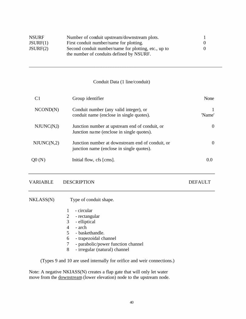
NSURF Number of conduit upstream/downstream plots. 1JSURF(1) First conduit number/name for plotting. 0JSURF(2) Second conduit number/name for plotting, etc., up to 0

the number of conduits defined by NSURF.

________________________________________________________________________________

Conduit Data (1 line/conduit)

C1 Group identifier None

NCOND(N) Conduit number (any valid integer), or 1conduit name (enclose in single quotes). 'Name'

NJUNC(N,l) Junction number at upstream end of conduit, or 0Junction name (enclose in single quotes).

NJUNC(N,2) Junction number at downstream end of conduit, or 0junction name (enclose in single quotes).

Q0 (N) Initial flow, cfs [cms]. 0.0


NKLASS(N) Type of conduit shape.

1 - circular2 - rectangular3 - elliptical4 - arch5 - baskethandle.6 - trapezoidal channel7 - parabolic/power function channel8 - irregular (natural) channel

(Types 9 and 10 are used internally for orifice and weir connections.)

Note: A negative NKIASS(N) creates a flap gate that will only let watermove from the downstream (lower elevation) node to the upstream node.

41

AFULL(N) Cross sectional area of conduit, ft2 [m2] 0.0enter only for types 4 and 5. (Geometricproperties for types 4 and 5 may be found in Section6 of the main SWMM User's Manual.)

DEEP(N) Vertical depth (diameter for type 1) 0.0of conduit, ft [m]. Not required for type 8.

WIDE(N) Maximum width of conduit, ft [m] 0.0Bottom width for trapezoid, ft [m]Top width for parabolic, ft [m]Not required (N.R.) for types 1 and 8.

LEN(N) Length of conduit, ft [m] 0.0 for type 8, enter it here for reference and also enter in data group C3.

Note: A negative LEN(N) creates a flap gate that will only let water move from the upstream (higher elevation) node to the downstream node.

ZP (N, 1) Invert of conduit at NJUNC(N,1), ft [m] 0.0


ZP(N, 2) Invert of conduit at NJUNC(N,2), ft [m] 0.0

ROUGH(N) Manning coefficient (not includes entrance, exit, 0.014expansion, and contraction losses).

N.R. for type 8. Uses XNCH in data group C2.

STHETA(N) Slope of one side of trapezoid. Required only for 0.0type - 6, (horizontal/vertical; 0 - vertical walls).For type 7, the channel exponent( 2.0, 3.0, etc.).For type 8, the cross-section identification number(SECNO, group C3) of the cross section used forthis EXTRAN channel. Unlike HEC-2, EXTRAN uses onlya single cross section to represent a naturalchannel reach for type 8 channels. A negative

STHETA(N) will eliminate the printing of the dimension-less curves associated with each natural channel or

42

power-function channel.

SPHI(N) Slope of other side of trapezoid. Required only for 0.0type - 6, (horizontal/vertical; 0 - vertical walls).The average channel slope for type 8. This slopeis used only for developing a rating curve forthe channel. Routing calculations use invertelevation differences divided by length.

(Following three fields only needed when KMLAG = 1 in B0 card.)

ENTRANCE Entrance loss coefficient 0.0

EXIT Exit loss coefficient 0.0

OTHER Other minor loss coefficient 0.0

SFACTOR Pipe extension factor 1.0

____________________________________________________________________________

The C2 (NC) or NH, C3 (Xl), and C4 (GR) data lines for any type 8 conduits follow as a groupafter all Cl lines have been entered. The sequence for channels must be in the same order as theearlier sequence of type-8 Cl-lines.


Data groups C2, C3 and C4 correspond to HEC-2 lines NC, Xl'and GR. HEC-2 input may beused directly if desired. Lines may be identified either by EXTRAN identifiers (C2, C3, C4) orHEC-2 identifiers (NC, Xl, GR). NH line is for multi-Manning’s n option. When more thanthree Manning’s n are required for a given cross-section, NH line, rather than C2 line, shouldbe prepared.

Channel Roughness

This is an optional data line that permanently modifies the Manning's roughness coefficients (n)for the remaining natural channels. This data group may repeated for later channels. It must beincluded for the first natural channel-modeled.

C2 or NC Group identifier None

XNL n for the left overbank. 0.0= 0.0, No change,

43

> 0.0, New Manning's n.

XNR n for the right overbank. 0.0= 0.0, No change,> 0.0, New Manning's n.

XNCH n for the channel. 0.0= 0.0, No change,> 0.0, New Manning's n.

Note, XNCH is used to develop normalized flow routing curves.

Or

NH Group identifier for more than three Manning’s n channel none

NXNL left bank number of Manning’s n 1

NXNR right bank number of Manning’s n 1

XNL1(1) the first Manning’s n on left bank 0.0

XNL1(2) the second Manning’s n on left bank 0.0

.

.

XNL1(NXNL) the NXNL Manning’s n on left bank 0.0

XNR1(1) the first Manning’s n on right bank 0.0

XNR1(2) the second Manning’s n on right bank 0.0

.

.

.

44

XNR1(NXNR) the NXNR Manning’s n on right bank 0.0

XNCH Main channel Manning’s n 0.0

Cross Section Data

Required for each type 8 conduit in earlier Cl data lines.Enter pairs of C3 and C4 lines in same sequence as appearanceof corresponding type 8 conduit in earlier Cl lines.

C3 or Xl Group identifier None

SECNO Cross section identification number. 1

NUMST Total number of stations on the following 0C4 (GR) data group lines. NUMST must be < 99.


STCHL The station of the left bank of the channel, 0.0ft [m]. Must be equal to one of the STA(N)on the C4 (GR) data lines.

(enter NXNL coordinates sequentially here if NH line prepared)

STCHR The station of the right bank of the channel, 0.0ft [m]. Must be equal to one of the STA(N)on the C4 (GR) data lines.

(enter NXNR coordinates sequentially here if NH line prepared)

XLOBL Not required for EXTRAN (enter 0.0). 0.0

XLOBR Not required for EXTRAN (enter 0.0). 0.0

LEN(N) Length of channel reach represented 0.0 by this cross section, ft [m].

45

PXSECR Factor to modify the horizontal dimensions 0.0for a cross section. The distances between adjacent C4 (GR) stations

(STA) are multiplied by this factor to expand or narrow a cross section. The STA of the first C4 (GR) point remains the same. The factor can apply to a repeated cross section or a current one. A factor of 1.1 will increase the horizontal distance between the C4 (GR) stations by 10 percent. Enter 0.0 for no modification.

PSXECE Constant to be added (+ or -) to C4 (GR) 0.0elevation data on next C4 (GR) line. Enter0.0 to use C4 (GR) values as entered.

Cross-Section Profile

Required for type 8 conduits in data group Cl.Enter C3 and C4 lines in pairs.

C4 or GR Group identifier None

EL(l) Elevation of cross section at STA(l). May be 0.0positive or negative, ft [m].

STA(1) Station of cross section 1, ft [m]. 0.0

EL(2) Elevation of cross section at STA(2), ft [m]. 0.0

STA(2) Station of cross section 2, ft [m]. 0.0

Enter NUMST elevations and stations to describe the cross section. Enter 5 pairs of elevationsand stations per data line. (Include group identifier, C4 or GR, on each line.) Stations should bein increasing order progressing from left to right across the section. Cross section data aretraditionally oriented looking downstream (HEC, 1982).

Junction Data (1 line/junction.)


Dl Group identifier None

46

JUN(J) Junction number (any valid integer), or 0junction name (enclose in single quotes).

GRELEV(J) Ground elevation, ft [m]. 0.0

Z(J) Invert elevation, ft [m]. 0.0

QINST(J) Net constant flow into junction, cfs [m3 /s] 0.0Positive indicates inflow.Negative indicates withdrawl or loss.

Y0(J) Initial water elevation, ft [m] Z(J)

Storage Junctions

Note: Each storage junction must also have beenentered in the junction data (Group DI).

El Group identifier None

JSTORE(I) Junction number containing storage facility, or 0junction name (enter in single quotes).

ZTOP(I) Junction crown elevation (must be higher than 0.0____________________________________________________________________________________


crown of highest pipe connected to thestorage junction), ft [m].

ASTORE(J) . Storage volume per foot (or meter) of d I pth 0.0(i.e., constant surface area) ft3/ft [m3 /m].

Set ASTORE(J) < 0 to indicate a variable-area storage junction.

NUMST required only if ASTORE < 0.

NUMST Total number of stage/storage area points 0 on following E2 data lines. NUMST < 99. Enter a value of -2 for NUMST to generate area vs. stage using a power function, A = a depthb.

47

____________________________________________________________________________

Follow El line with E2 line(s) only if ASTORE < 0,or NUMST equals -2 on line El.

Variable-Area Storage Junction, Stage vs. Surface Area Points

E2 Group identifier None

QCURVE(N,1,1) Surface area of storage junction at depth point 0.01, acres [hectares]. If NUMST equals -2 this isthe coefficient of the power function.

QCURVE(N,2,1) Elevation at point 1, ft [m]. 0.0If NUMST equals -2 this is the exponent of thepower function. This is the last value enteredif NUMST equals -2.

QCURVE(N,1,2) Surface area of storage junction at depth point 0.02, acres [hectares].

QCURVE(N,2,2) Elevation at point 2, ft [m]. 0.0 .

.

.

.


Continue entering total of NUMST (data group El) area-stage points.Use only one E2 group identifier for the E2 data group. If more than one line is required leave thefirst two columns blank.

Orifice Data (60 Max.)

Fl Group identifier None

NJUNC(N,l) Junction number containing orifice, or Nonejunction name (enter in single quotes).

NJUNC(N,2) Junction number to which orifice discharges, or Nonejunction name (enter in single quotes).

48

NKIASS(N) Type of orifice. 11 - side outlet,2 - bottom outlet,

-1 - time-history side outlet orifice,with data entered on data group F2.

-2 - time-history bottom outlet orifice,with data entered on data group F2.

AORIF(I) Orifice area, ft2 [m 2 ]. 0.0

CORIF(I) Orifice discharge coefficient. 1.0

ZP(I) Orifice invert 0.0(define only for side outletorifices), ft [m].

Time-History Orifice Data

Each F2 line follows the appropriate Fl line.

F2 Group identifier None

NTIME Number of data points to describe the time 1____________________________________________________________________________________


history of the orifice (50 max.).

VORIF(I,1,1) First time, hours, that the orifice discharge 0.0coefficient and area change values from intialsettings of group Fl above. Time zero refers tobeginning (midnight) of beginning day of simulation.E.g., VORIF(I,1,1) = 22.0 means first change inorifice setting occurs at 10:00 p.m. on first day ofsimulation. Increase hours past 24 (e.g., 25, 26)for multi-day simulations.

VORIF(I,1,2) First new value of orifice discharge coefficient. 0.0

49

VORIF(I,1,3) First new value of orifice area. 0.0...

Enter NTIME values of time/coefficient/area. Only one F2 group identifier isrequired, on the first data line. Subsequent lines (if required) should not include F2identifier.

Weir Data (1 line/weir, 60 Max.)

Gl Group identifier None

NJUNC(N,1) Junction number at which weir is located, or 0Junction name (enter in single quotes).

NJUNC(N,2) Junction number to which weir discharges, or 0Junction name (enter in single quotes).

Note: To designate outfall weir, set NJUNC(N,2)equal to zero or (one space between quotes).

KWEIR(I) Type of weir. 1

1 = transverse


2 = transverse with tide gate, 3 = side flow, 4 = side flow with tide gate.

YCREST(I) Elevation of weir crest, ft [m]. 0.0

YTOP(I) Elevation of top of weir opening(surcharge level) ft [m].

WLEN(I) Weir length, ft [m]. 0.0

COEF(I) Coefficient of discharge for weir. 1.0

50

Pump Data (1 line/pump, 20 Max.)

Note: ONLY ONE PIPE CAN BE CONNECTED TO A TYPE 1 PUMP NODE.

Hl Group identifier None

IPTYP(I) Type of pump. 11 = off-line pump with wet well (program will

set pump junction invert to -100),2 = in-line lift pump,3 = three-point head-discharge pump curve.

NJUNC(N,l) Junction number being pumped, or 0Junction name (enter in single quotes).

NJUNC(N,2) Pump discharge goes to this junction number, or 0junction name (enter in single quotes).

PRATE(I,l) Lower pumping rate, ft 3 /s [m 3 /s]. 0.0


PRATE(I,2) Mid-pumping rate, ft3 /s [m 3 /s]. 0.0

PRATE(I,3) High pumping rate, ft 3 /s [m3/s]. 0.0

VRATE (I, 1) If IPTYP = 1 enter the wet well volume for 0.0 mid-rate pumps to start, ft3 [m3 ]. If IPTYP = 2 enter the junction depth for mid-rate pumps to start, ft [m]. If IPTYP = 3 enter the head difference (head at junction downstream of pump minus and head at junction upstream of pump) associated with the lowest pumping rate, ft [m]. (This will be the highest head difference.)

51

VRATE (I, 2) If IPTYP = 1 enter the wet well volume for 0.0 high-rate pumps to start, ft3 [m3] . If IPTYP = 2 enter the junction depth for high-rate pumps to start, ft [m] . If IPTYP = 3 enter the head difference associated with the mid-pumping rate, ft [m]

Non-zero VRATE(I,3) and VWELL(I) required only if IPTYP = 1 or 3.

VRATE(I,3) If IPTYP = 1 enter total wet well capacity, ft3 [m3 ] 0.0 If IPTYP = 3 then enter the head difference associated with highest pumping rate, ft [m]. (This will be the lowest head difference.)

VWELL(I) If IPTYP = 1 then enter initial wet well volume, ft3 [m3 ] 0.0 If IPTYP = 3 then enter the intial depth in pump inflow Junction, ft [m]

Enter PON(I) and POFF(I) if IPTYP = 3

PON(I) Depth in pump inflow junction to turn pump on, 0.0ft [m].


POFF(I) Depth in pump inflow junction to turn pump 0.0off, ft [m].

Note: for groups Il and I2, enter junction name in single quotes ifalphanumeric option is being used.

Outfalls Without Tide Gates (1 line/outfall, 25 Max.)

Note: ONLY ONE CONNECTING CONDUIT IS PERMITTED TO AN OUTFALLNODE.

52

I1 Group identifier None

JFREE(I) Number/name of outfall junction without tide gate 0(no back-flow restriction).

NBCF(I) Type of boundary condition, from sequence of 1data group J1 - J4.

Outfalls with Tide Gates (1 line/outfall, 25 max.)

Note: ONLY ONE CONNECTING CONDUIT IS PERMITTED TOAN OUTFALL NODE.

I2 Group identifier None

JGATE(I) Number/name of outfall junction with tide gate 0(back-flow not allowed).

NBCG(I) Type of boundary condition, from sequence of 1data groups Jl - J4.


Boundary Condition Information

Note: Repeat sequence of data groups Jl-J4 for up to 20 different boundary conditions.Appearance in sequence (e.g., first, second... fifth...) determines value for NBCF and NBCG indata groups Il and I2.

J1 Group identifier None

NTIDE(I) Boundary condition index. 11 = No water surface at outfalls (elevated discharge),2 = Controlling water surface at outfall

at constant elevation Al (group J2), ft [m],

53

Types 3, 4 and possibly 5 are used for tidal variations at outfall.

3 = Tide coefficients (Group J2) provided by user,4 = Program will compute tide coefficients,

5 = Stage-history of water surface elevations input by user. Program uses linear interpolation between data points.

Stage and/or Tidal Coefficients

Note: NOT REQUIRED (OMIT) IF NTIDE(I) = 1 OR 5 ON DATA GROUP Jl.


Al(I) First tide coefficient, ft [m]. 0.0

W(I) Tidal period, hours. 0.0Required only if NTIDE(I) = 3 or 4.

Note: NEXT SIX FIELDS NOT REQUIRED UNLESS NTIDE(I) = 3


A2(I) Second tide coefficient, ft [m]. 0.0

A3(I) Third tide coefficient, ft [m]. 0.0

A4(I) Fourth tide coefficient, ft [m]. 0.0

A5(I) Fifth tide coefficient, ft [m]. 0.0

A6(I) Sixth tide coefficient, ft [m]. 0.0

A7(I) Seventh tide coefficient, ft [m]. 0.0

Tidal/Stage Information

54

REQUIRED ONLY IF NTIDE = 4 OR 5


K0 Type of tidal input.= 0, Input is in the form of a time series 0

of NI tidal heights. This parameter is notused if NTIDE equals 5.

=1, Input is in the form of the high and lowwater values found in the tide tables, (HHW,LLW, LHW, and HLW). NI must be 4.

NI Number of information points. 4

NCHTID Tide information print control. 1= 0, Do not print information,= 1, Print information on tide coefficients

or stage history.

DELTA Convergence criterion for fitting of tidal 0.005function, ft [m]. Not required for NTIDE = 5.


Time and stage information

REQUIRED IF NTIDE = 4 OR 5


TT(l) - Time of day, first information point, hours. 0.0(Increase hours past 24 if necessary.)

YY(I) Tide/stage at time above, ft [m]. 0.0

TT(2) Time of day, second information points, hours. 0.0

YY(2) Tide/stage, at time above, up to number 0.0

55

of points as defined by NI, ft [m].

Note: Enter 5 pairs of time and stage information per data line.(Repeat group identifier on each line.)

___________________________________________________________________________

User Input Hydrographs

IF NJSW = 0 (GROUP B3), SKIP DATA GROUPS Kl, K2 AND K3

Kl Group identifier None

NINC Number of input nodes and flows per line 1in group K3.

56


Hydrograph Nodes

K2 Group identifier None

JSW(1) First input node number for line hydrograph, or 0node name (enter in single quotes).

JSW(2) Second input node number for line hydrograph, or 0 node name (enter in single quotes).

Enter NINC nodes per line until NJSW nodes are entered.(Repeat group identifier on each line.)

User Input Hydrographs

K3 Group identifier None

TEO Time of day, decimal hours. 0.0

QCARD(l,l) F13w ratq for first input node, JSW(l), 0.0ft3 [m3 ].

QCARD(2,1) Flsw rat I for second input node, JSW(2), 0.0ft3 [m3 ].

Enter TEO plus NINC flows per line until NJSW flows are entered. Enter TEOonly on first of multiple ("wrapped around") lines and do not include group identifier K3on lines that are "wrapped around.' Repeat the sequence for each TEO time. Times donot have to be evenly spaced; linear interpolation is used to interpolate between entries.The last K3 line will signal the end of the user hydrograph input. The last TEO valueshould be > length of simulation. Increase TEO past 24 for multi-day simulations.

END OF EXTRAN DATA INPUT

Control now returns to the Executive Block of SWMM.

If no more SWMM blocks are to be called, end input with $ENDPROGRAMin columns 1-11.

57

Example:

* ==========================================================================* EXAMPLE OF SWMM INPUT** ===========================================================================* NBLOCKS INBLK1 OUTBLK1 INBLK2 OUTBLK2SW 2 8 12 12 0MM 6 10 11 13 14 15 16@ 8 'EXAMPL.WPX'@ 11 'EXAMPL.HOT'@ 12 'EXAMPL.INT'@ 15 'EXAMPL.SMX'@ 16 'EXAMPL.PLT'$COMBINEA1 11B1 ' A1=11 GENERATE HYDROGRAPH FROM WPX FILE 'B1 ' MAKE SWMM INTERFACE FILE '*$EXTRAN* ALPHAA1 ' EXISTING CONDITION 'A1 ' DESIGN STORM EVENT'* ISOL KSUPERB0 2 0 1BB 1 0B1 86400 1.00 0.0 1 3600 3600 0B2 0 0 12.6 30 0.05* H-prnt Q-prnt H-plot Q-plotB3 3 2 3 2 0 0 1B4 101005 100022 101007B5 1101005 1101015B6 101005 100022 101007B7 1101005 1101015**=============================================** 1. ORIENT PARK SYSTEMK_ent K_exit K_orther Stretch*=============================================** TWC1 1101005 0101005 0100022 0.0 1 0.0 5.00 0.00 80.0 4.95 4.85 0.024 0.0 0.0 0.5 1.0 0.0 1.0C1 2101005 0101005 0100022 0.0 1 0.0 5.00 0.00 80.0 4.95 4.85 0.024 0.0 0.0 0.5 1.0 0.0 1.0* WEIR 0101007 0101005C1 9101010 0101010 0101007 0.0 8 0.0 0.00 0.00 400.0 8.95 6.95 0.0 –9101010 0.0030 0.00.0 0.0 1.0*----BROADWAYC1 1101015 0101015 0101010 0.0 1 0.0 7.50 0.00 150.0 9.05 8.95 0.009600.0000 0.0000 0.5 1.0 0.0 1.0* UPGRADEC1 1101025 0101025 0101015 0.0 1 0.0 7.00 0.00 450.0 9.15 9.05 0.012000.0000 0.0000 0.5 1.0 0.0 1.0* UPGRADEC1 1101030 0101030 0101025 0.0 1 0.0 6.50 0.00 50.0 9.20 9.15 0.012000.0000 0.0000 0.5 1.0 0.0 1.0C1 9101035 0101035 0101030 0.0 8 0.0 0.00 0.00 400.0 14.80 9.20 0.00000 -9101035 0.0110 0.0 0.0 0.0 1.0*----76TH ST. PICTURE ERCP*C1 1101040 0101040 0101035 0.0 2 0.0 4.00 8.00 40.0 15.30 14.80 0.012000.0000 0.0000 0.5 1.0 0.0 1.0C1 9101045 0101045 0101040 0.0 8 0.0 0.00 0.00 200.0 16.36 15.30 0.00000 -9101045 0.0080 0.0 0.0 0.0 1.0*----75TH ST.C1 1101050 0101050 0101045 0.0 2 0.0 4.00 8.00 40.0 16.57 16.36 0.012000.0000 0.0000 0.5 1.0 0.0 1.0C1 9101055 0101055 0101050 0.0 8 0.0 0.00 0.00 190.0 17.73 16.57 0.00000 -9101055 0.0010 0.0 0.0 0.0 1.0*----MISSOURI ST. L=? 115 OR 40C1 1101060 0101060 0101055 0.0 2 0.0 4.00 8.00 40.0 18.23 17.73 0.012000.0000 0.0000 0.5 1.0 0.0 1.0

58

C1 9101065 0101065 0101060 0.0 8 0.0 0.00 0.00 160.0 19.70 18.23 0.00000 -9101065 0.0030 0.0 0.0 0.0 1.0*----ORIENT RD.C1 1101070 0101070 0101065 0.0 2 0.0 4.00 8.00 50.0 19.75 19.70 0.012000.0000 0.0000 0.5 1.0 0.0 1.0C1 9101075 0101075 0101070 0.0 8 0.0 0.00 0.00 150.0 20.25 19.75 0.00000 -9101075 0.0050 0.0 0.0 0.0 1.0*----FIRST ASSEMBLY OF GODC1 1101080 0101080 0101075 0.0 1 0.0 3.00 0.00 37.0 20.43 20.25 0.012000.0000 0.0000 0.5 1.0 0.0 1.0C1 1101090 0101090 0101080 0.0 1 0.0 3.00 0.00 62.0 20.51 19.89 0.012000.0000 0.0000 0.5 1.0 0.0 1.0C1 1101095 0101095 0101090 0.0 3 0.0 4.00 2.50 112.0 20.90 20.43 0.012000.0000 0.0000 0.5 1.0 0.0 1.0C1 1101105 0101105 0101095 0.0 1 0.0 3.00 0.00 285.0 23.69 20.94 0.018000.0000 0.0000 0.5 1.0 0.0 1.0*----21ST ST. NEW SURVEYC1 1101115 0101115 0101105 0.0 3 0.0 2.50 4.42 64.5 25.09 25.00 0.034000.0000 0.0000 0.5 1.0 0.0 10.0C1 2101115 0101115 0101105 0.0 3 0.0 2.67 4.33 64.5 25.60 25.48 0.034000.0000 0.0000 0.5 1.0 0.0 10.0C1 9101120 0101120 0101115 0.0 6 0.0 13.90 6.20 1000.0 24.89 24.50 0.040001.1300 1.1300 0.0 0.0 0.0 1.0* PROPOSED DETENTION PONDS* WEIR 120 117* WEIR 117 115*----RHODE ISLAND 48"CMP L=230'C1 1101127 0101127 0101120 0.0 1 0.0 4.00 0.00 230.0 26.12 24.89 0.024000.0000 0.0000 0.5 1.0 0.0 10.0*----VERMONT DRIVEC1 1101140 0101140 0101127 0.0 1 0.0 2.50 0.00 36.7 27.12 27.11 0.012000.0000 0.0000 0.5 1.0 0.0 2.0C1 9101145 0101145 0101140 0.0 6 0.0 13.10 3.00 500.0 28.30 27.12 0.040002.3300 2.3300 0.0 0.0 0.0 1.0C1 9101150 0101150 0101145 0.0 8 0.0 0.00 0.00 550.0 29.63 28.30 0.00000 -9101150 0.0270 0.0 0.0 0.0 1.0*----CORPOREX PARK DRIVEC1 1101160 0101160 0101150 0.0 3 0.0 4.00 6.33 100.0 29.93 29.63 0.012000.0000 0.0000 0.5 1.0 0.0 1.0C1 2101160 0101160 0101150 0.0 3 0.0 4.00 6.33 100.0 29.93 29.63 0.012000.0000 0.0000 0.5 1.0 0.0 1.0*----CITICORP BLVDC1 1101170 0101170 0101160 0.0 1 0.0 4.00 0.00 120.0 30.10 30.00 0.012000.0000 0.0000 0.5 1.0 0.0 1.0*----BRANCHC1 1101146 0101146 0101150 0.0 1 0.0 2.50 0.00 45.0 30.90 30.64 0.012000.0000 0.0000 0.5 1.0 0.0 1.0C1 1101148 0101148 0101150 0.0 3 0.0 1.58 2.50 36.0 30.90 30.68 0.012000.0000 0.0000 0.5 1.0 0.0 1.0C1 1101161 0101161 0101160 0.0 1 0.0 2.00 0.00 24.0 31.50 31.40 0.012000.0000 0.0000 0.5 1.0 0.0 1.0C1 1101163 0101163 0101160 0.0 1 0.0 1.50 0.00 24.0 31.50 31.40 0.012000.0000 0.0000 0.5 1.0 0.0 1.0C1 1101171 0101171 0101160 0.0 1 0.0 2.50 0.00 24.0 30.70 30.60 0.012000.0000 0.0000 0.5 1.0 0.0 10.0*----BRANCH (Tributary O2)C1 1101210 0101210 0101120 0.0 1 0.0 2.00 0.00 72.0 28.84 28.15 0.012000.0000 0.0000 0.5 1.0 0.0 1.0C1 1101220 0101220 0101210 0.0 1 0.0 1.25 0.00 70.0 29.36 28.84 0.012000.0000 0.0000 0.5 1.0 0.0 1.0C1 2101220 0101220 0101210 0.0 1 0.0 1.25 0.00 66.0 29.74 29.64 0.012000.0000 0.0000 0.5 1.0 0.0 1.0C1 1101235 0101235 0101220 0.0 1 0.0 1.25 0.00 140.0 30.08 29.49 0.024000.0000 0.0000 0.5 1.0 0.0 1.0C1 1101245 0101245 0101235 0.0 1 0.0 2.00 0.00 130.0 31.85 31.21 0.012000.0000 0.0000 0.5 1.0 0.0 1.0*----BRANCHC1 9101430 0101430 0101425 0.0 6 0.0 12.00 1.50 687.0 29.93 29.63 0.040001.4000 1.4000 0.0 0.0 0.0 1.0C1 9101435 0101435 0101430 0.0 6 0.0 13.00 6.00 250.0 30.55 29.33 0.040001.2000 1.2000 0.0 0.0 0.0 1.0

59

C1 1101445 0101445 0101435 0.0 1 0.0 1.50 0.00 38.0 30.99 30.22 0.024000.0000 0.0000 0.5 1.0 0.0 1.0C1 1101450 0101450 0101445 0.0 1 0.0 1.50 0.00 38.0 30.86 30.75 0.012000.0000 0.0000 0.5 1.0 0.0 1.0*----BRANCH-BETWEEN ORIENT PARK & JUDSON CREEK* TWC1 1101505 0101505 0100025 0.0 1 0.0 4.00 0.00 50.0 22.86 22.76 0.012000.0000 0.0000 0.5 1.0 0.0 1.0C1 1101520 0101520 0101505 0.0 1 0.0 5.00 0.00 120.0 21.08 21.21 0.024000.0000 0.0000 0.5 1.0 0.0 1.0*- WEIR 0101535 0101520*** CHANNEL IMPROVEMENTS UP TP 1070* --- Natural Channel Da 1005C2 0.040 0.040 0.035C3 9101010 6 100.00 130.00 0.00 0.00 400.00 0.00 0.00C4 21.500 99.900 15.500 100.000 10.300 110.000 10.300 120.000 15.500 130.000C4 21.500 130.100* ---- Natural Channel Da 1030C2 0.040 0.040 0.035C3 9101035 7 100.00 130.10 0.00 0.00 400.00 0.00 0.00C4 29.500 99.900 19.500 100.000 14.400 107.600 13.900 112.600 14.600 117.100C4 19.200 130.100 29.200 130.200* ---- Natural Channel Da 1040C2 0.040 0.040 0.035C3 9101045 7 100.00 128.00 0.00 0.00 200.00 0.00 0.00C4 31.400 99.900 21.400 100.000 17.300 105.000 17.100 113.000 18.200 121.000C4 22.500 128.000 32.500 128.100* --*-- Natural Channel Da 1050C2 0.040 0.040 0.035C3 9101055 7 100.00 120.00 0.00 0.00 190.00 0.00 0.00C4 31.700 99.900 21.700 100.000 18.500 108.600 18.200 112.300 18.500 116.000C4 22.000 120.000 32.000 120.100* ----Natural Channel Da 1060C2 0.040 0.040 0.035C3 9101065 7 100.00 123.80 0.00 0.00 160.00 0.00 0.00C4 32.100 99.900 22.100 100.000 18.900 105.700 18.600 113.050 18.900 120.400C4 21.900 123.800 31.900 123.900* CHANNEL IMPROVEMENTS UP TO D/S OF ORIENT ROAD* ---- Natural Channel Da 1070C2 0.040 0.040 0.040C3 9101075 7 100.00 122.00 0.00 0.00 150.00 0.00 0.00C4 33.500 99.900 23.500 100.000 20.000 103.000 19.700 110.000

60

19.700 117.000C4 23.600 122.000 33.600 122.100* ---- Natural Channel Da 1145C2 0.040 0.040 0.040C3 9101150 7 100.00 115.50 0.00 0.00 550.00 0.00 0.00C4 40.600 99.900 30.600 100.000 28.800 103.700 28.200 107.900 28.700 112.100C4 30.500 115.500 40.500 115.600*=================================================**D1 0100025 99 22.76 0 27.00D1 0100026 99 24.45 0 28.00D1 0100027 99 24.45 0 28.00*------------------------------------------** SOUTH SYSTEM* Orient Park Outfall*------------------------------------------*D1 0101005 99 4.95 0 9.70D1 0101007 99 6.95 0 9.70D1 0101010 99 8.95 0 9.70D1 0101015 99 9.05 0 9.70*D 0101020 99 9.15 0 9.70D1 0101025 99 9.15 0 9.70D1 0101030 99 9.20 0 9.70D1 0101035 99 14.80 0 14.80D1 0101040 99 15.30 0 15.40D1 0101045 99 16.36 0 16.46D1 0101050 99 16.57 0 16.57D1 0101055 99 17.73 0 17.73D1 0101060 99 18.23 0 18.39D1 0101065 99 19.70 0 19.70D1 0101070 99 19.75 0 19.85D1 0101075 99 20.25 0 20.25D1 0101080 99 20.43 0 20.53D1 0101090 99 20.43 0 20.53D1 0101095 99 20.90 0 21.00D1 0101105 99 23.69 0 23.79D1 0101115 99 24.50 0 24.50** PROPOSED POND LOCATIOND1 0101117 99 24.50 0 24.50*D1 0101120 99 24.89 0 24.99D1 0101127 99 26.12 0 26.12D1 0101140 99 27.12 0 27.12D1 0101145 99 28.30 0 28.40D1 0101146 99 30.90 0 32.30D1 0101147 99 31.99 0 32.30D1 0101148 99 30.90 0 32.30D1 0101149 99 31.54 0 32.30D1 0101150 99 29.63 0 32.30D1 0101151 99 32.40 0 32.50D1 0101160 99 29.93 0 32.30D1 0101161 99 31.50 0 32.30D1 0101162 99 31.50 0 32.30D1 0101163 99 31.50 0 32.30D1 0101164 99 31.50 0 32.30*D 0101165 99 27.90 0 32.30D1 0101170 99 30.10 0 32.30D1 0101171 99 30.70 0 32.30D1 0101172 99 32.76 0 32.86* Trib. O2D1 0101210 99 28.84 0 28.94D1 0101215 99 29.36 0 29.46D1 0101220 99 29.36 0 29.34D1 0101235 99 30.08 0 30.18

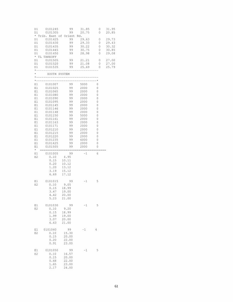
61

D1 0101245 99 31.85 0 31.95D1 0101305 99 20.75 0 20.85* Trib. East of Orient Rd.D1 0101425 99 29.63 0 29.73D1 0101430 99 29.33 0 29.43D1 0101435 99 30.22 0 30.32D1 0101445 99 30.75 0 30.85D1 0101450 99 28.98 0 29.08* TL TAKEOFFD1 0101505 99 21.21 0 27.00D1 0101520 99 21.08 0 27.00D1 0101535 99 25.69 0 25.79*----------------------------------* SOUTH SYSTEM*----------------------------------*---------------------------------*E1 0101007 99 5000 0E1 0101025 99 2000 0E1 0101065 99 2000 0E1 0101080 99 2000 0E1 0101090 99 2000 0E1 0101095 99 2000 0E1 0101145 99 2000 0E1 0101146 99 2000 0E1 0101148 99 2000 0E1 0101150 99 5000 0E1 0101161 99 2000 0E1 0101163 99 2000 0E1 0101171 99 2000 0E1 0101210 99 2000 0E1 0101215 99 2000 0E1 0101220 99 2000 0E1 0101235 99 6000 0E1 0101425 99 2000 0E1 0101505 99 2000 0* ====================================E1 0101005 99 -1 6E2 0.10 4.95 0.15 10.11 0.20 10.12 1.20 13.12 3.19 15.12 6.69 17.12

E1 0101015 99 -1 5E2 0.10 9.05 0.15 18.99 3.47 19.00 4.42 20.00 5.23 21.00

E1 0101030 99 -1 5E2 0.10 9.20 0.15 18.99 1.99 19.00 3.07 20.00 6.63 21.00

E1 0101040 99 -1 4E2 0.10 15.30 0.15 20.00 0.20 22.00 0.91 23.00

E1 0101050 99 -1 5E2 0.10 16.57 0.15 20.00 0.68 22.00 1.65 23.00 2.17 24.00

62

E1 0101060 99 -1 5E2 0.10 18.23 0.15 20.00 0.35 22.00 1.24 23.00 2.02 24.00

E1 0101075 99 -1 7E2 0.10 20.25 0.15 21.99 0.20 22.00 0.90 23.00 4.88 24.00 8.86 25.00 11.44 26.00*E1 0101105 99 -1 6E2 0.10 23.69 0.20 25.99 1.00 26.00 1.50 28.00 2.00 30.00 2.50 32.00* REVISED FOR PROPOSED DETENTION PONDE1 0101115 99 -1 6E2 0.10 24.50 0.15 28.99 0.29 29.00 0.93 30.00 1.67 31.00 1.72 32.00* PROPOSED DETENTION POND BETWEEN RHODE ISLAND & 21ST AVE.E1 0101117 99 -1 6E2 3.70 24.50 4.00 26.50 4.30 28.50 5.93 30.00 8.67 31.00 11.72 32.00

E1 0101120 99 -1 6E2 0.10 24.89 0.15 28.99 0.16 29.00 0.83 30.00 1.73 31.00 2.46 32.00

E1 0101127 99 -1 5E2 0.10 26.12 0.15 29.99 0.20 30.00 0.91 31.00 1.95 32.00

E1 0101140 99 -1 4E2 0.10 27.12 0.15 30.99 0.30 31.00 1.37 32.00

E1 0101147 99 -1 4E2 0.51 31.99 0.81 33.00 0.91 36.00 0.91 38.00

E1 0101149 99 -1 4E2 1.05 31.54 1.05 33.00 1.10 34.23

63

1.32 35.00

E1 0101151 99 -1 4E2 0.10 32.40 3.22 33.00 6.04 34.00 8.74 35.00

E1 0101160 99 -1 4E2 0.10 29.93 25.22 31.00 36.95 33.00 50.22 35.00

E1 0101162 99 -1 5E2 1.30 31.5 1.59 33.00 2.67 34.00 3.37 35.00 3.50 36.00

E1 0101164 99 -1 4E2 1.00 31.50 1.34 33.00 1.88 34.00 2.00 36.00

E1 0101170 99 -1 4E2 0.10 30.10 0.51 32.00 2.19 34.00 9.81 35.00

E1 0101172 99 -1 3E2 0.50 32.76 0.98 34.00 1.00 37.00

E1 0101245 99 -1 5E2 0.10 31.85 0.15 32.50 0.63 34.00 2.11 35.00 4.16 36.00

E1 0101305 99 -1 4E2 0.10 20.75 0.17 24.00 1.43 25.00 3.87 26.00

E1 0101450 99 -1 4E2 0.10 28.98 0.49 30.00 0.82 31.00 3.85 32.00

E1 0101520 99 -1 7E2 0.10 21.08 0.15 24.90 0.20 25.00 0.52 26.00 2.50 27.00 4.81 28.00 11.25 29.00

E1 0101535 99 -1 4E2 0.10 25.69 0.15 28.00 0.22 29.00

64

0.30 30.00*-------------------------------------------** South system Orifice*-------------------------------------------**F1 0101147 0101147 0101146 1 2.40 0.6 0.00F1 0101149 0101149 0101148 1 1.69 0.6 0.00*-------------------------------------------** ORIENT PARK*-------------------------------------------*G1 8101007 0101007 0101005 1 9.20 99 14 3.1 1G1 7101015 0101015 0101010 1 19.00 99 18 2.6 1G1 7101025 0101025 0101015 1 19.00 99 24 2.6 1G1 7101030 0101030 0101025 1 19.00 99 22 2.6 1G1 7101040 0101040 0101035 1 21.99 99 28 2.6 1G1 7101050 0101050 0101045 1 22.42 99 24 2.6 1G1 7101060 0101060 0101055 1 22.35 99 24 2.6 1G1 7101070 0101070 0101065 1 24.20 99 24 2.6 1*-----------------------------------** CHURCH SITE ROAD OVERTOPPING WEIR* BASED ON SITE OBSERVATION RULE*3*-----------------------------------*G1 7101080 0101080 0101075 1 24.23 99 36 2.6 1G1 7101090 0101090 0101080 1 24.80 99 36 2.6 1G1 7101095 0101095 0101090 1 25.40 99 48 2.6 1G1 7101105 0101105 0101095 1 28.52 99 36 2.6 1G1 7101115 0101115 0101105 1 31.44 99 35 2.6 1* PROPOSED DETENTION & CONTROL STRUCTUREG1 8101120 0101120 0101117 1 26.00 99 20 3.1 1G1 8101117 0101117 0101115 1 28.00 99 20 3.1 1*G1 7101127 0101127 0101120 1 30.08 99 16 2.6 1G1 7101140 0101140 0101127 1 31.10 99 10 2.6 1G1 7101160 0101160 0101150 1 37.26 99 51 2.6 1G1 7101170 0101170 0101160 1 36.35 99 16 2.6 1*G1 6101147 0101147 0101150 1 36.00 99 50 2.6 1G1 6101149 0101149 0101150 1 34.23 99 50 2.6 1G1 7101151 0101151 0101145 1 32.50 99 50 2.6 1G1 7101162 0101162 0101160 1 35.00 99 50 2.6 1G1 7101164 0101164 0101160 1 35.00 99 50 2.6 1G1 7101172 0101172 0101160 1 36.45 99 50 2.6 1G1 7101235 0101235 0101120 1 34.00 99 50 2.6 1G1 6101245 0101245 0101151 1 35.30 99 50 2.6 1G1 8101305 0101305 0101075 1 20.75 22.75 1.4 3.31 1G1 7101305 0101305 0101075 1 24.29 99 50 2.6 1G1 7101127 0101127 0101425 1 31.00 99 50 2.6 1G1 8101127 0101127 0101425 1 29.74 99 0.8 3.1 2G1 6101535 0101535 0101520 1 29.50 99 50 2.6 1*- -------------------------*I1 0100024 1I1 0100025 2I1 0100026 3I1 0100027 4* J-CARD GROUP 1J1 5J3 0 3 1J4 0 2.5 15 2.5 240 2.5* J-CARD GROUP 2J1 5J3 0 3 1J4 0 27.0 15 27.0 240 27.0* J-CARD GROUP 3J1 5J3 0 3 1J4 0 27.0 15 27.0 240 27.0* J-CARD GROUP 4J1 5J3 0 3 1J4 0 28.0 15 28.0 240 28.0$ENDPROGRAM

65

APPENDIX A, OVERLAND FLOWMANNING'S N VALUES

Basin Type Recommended value Range of valuesConcrete 0.011 0.01 - 0.013Asphalt 0.012 0.01 - 0.015Bare Sand 0.010 0.010 -- 0.016Graveled Surface 0.012 0.012 - 0.030Bare Clay-loam (eroded) 0.012 0.012 - 0.033Fallow (no residue) 0.05 0.006 - 0.16Chisel Plow (<1/4 tons/acre residue) 0.07 0.006 - 0.17Chisel Plow (1/4 - 1 tons/acre residue) 0.18 0.07 -- 0.34Chisel Plow (1 - 3 tons/acre residue) 0.30 0.19 -- 0.47Chisel Plow (>3 tons/acre residue ) 0.40 0.34 -- 0.46Disk/Harrow (<1/4 tons/acre residue) 0.08 0.008 - 0.41Disk/Harrow (1/4 -1 tons/acre residue) 0.16 0.10 -- 0.25Disk/Harrow (1 - 3 tons/acre residue ) 0.25 0.14 -- 0.53Disk/Harrow (>3 tons/acre residue) 0.30 N/ANo Till (<1/4 tons/acre residue) 0.04 0.03 -- 0.07No Till (1/4 - 1 tons/acre residue) 0.07 0.01 -- 0.13No Till (1 - 3 tons/acre residue ) 0.30 0.16 -- 0.47Plow (fall) 0.06 0.02 -- 0.10Coulter 0.10 0.05 -- 0.13Range (natural) 0.13 0.01 -- 0.32Range (clipped) 0.08 0.02 -- 0.24Grass (bluegrass sod) 0.45 0.39 -- 0.63Short grass praire 0.15 0.10 -- 0.20Dense grass 0.24 0.17 -- 0.30Bermudagrass 0.41 0.30 -- 0.48Woods 0.45 N/A

66

APPENDIX B

CULVERT ENTRANCE LOSS COEFFICIENTSOUTLET CONTROL, FULL OR PARTIALLY FULL

Type of Structure and Design of Entrance Coefficient ke

Pipe, Concrete

Projecting from fill, socket end (groove-end) 0.2Projecting from fill, square cut end 0.5Straight headwall

Socket end of pipe (groove-end) 0.2Square-edge 0.5Rounded (radius = 1/12D) (Indexes 250, 251, 252, 253, 255) 0.2

Mitered to conform to fill slope (Indexes 272, 273, 274) 0.7End section conforming to fill slope' 0.5Beveled edges, 33.7o or 45o bevels 0.2Side- or slope-tapered inlet 0.2Straight sand-cement (Index 258) 0.3U-type with grate (Index 260) 0.7U-type (Index 261) 0.5Winged concrete (Index 266) 0.3U-type sand-cement (Index 268) 0.5Flared end concrete (Index 270) 0.5Side drain, mitered with grate (Index 273) 1.0

Pipe or Pipe-Arch, Corrugated Metal

Straight endwall--rounded (Radius=1/12 D) (Index 250) 0.2Projecting from fill (no headwall) 0.9Headwall or headwall and wingwalls, square-edge 0.5Mitered to conform to fill slope (Indexes 272, 273, 271) 0.7End section conforming to fill slope, paved or unpaved* 0.5Beveled edges, 33.7o or 45o bevels 0.2Side- or slope-tapered inlet 0.2

Box, Reinforced Concrete

Headwall parallel to embankment (no wingwalls) Square-edged on three edges 0.5

Rounded on three edges to radius of 1/12 barrel dimension, or beveled edges on three sides (Index 290) 0.2

67

APPENDIX B (continue)

CULVERT ENTRANCE LOSS COEFFICIENTSOUTLET CONTROL, FULL OR PARTIALLY FULL

Type of Structure and Design of Entrance Coefficient ke

Wingwalls at 30o to 75o to barrel Square-edged at crown 0.4 Crown edge rounded to radius of 1/12 barrel dimension, or

beveled top edge 0.2 Wingwalls at 10o to 25o to barrel, square-edged at crown 0.5 Wingwalls parallel (extension of sides)

Square edged at crown 0.7 Side- or slope-tapered inlet 0.2

_______________________________________

*End sections conforming to fill slope, made of either metal or concrete, are the sectionscommonly available from manufacturers. From limited hydraulic tests, they are equivalent inoperation to a headwall in both inlet and outlet control. Some end sections incorporating a closedtaper in their design have a superior hydraulic performance.

Note: Entrance head loss, g

VKH ee 2

2

=

Reference : USDOT, FHWA, HEC-5 (1965).

Date post:	14-Jun-2018
Category:	Documents
Upload:	hathien
View:	225 times
Download:	0 times

Hillsborough County SWMM4.31B User’s Manual · The Storm Water Management Model (SWMM) was...

Documents