Page 1

HSR Airframe Technical Review

Los Angeles, CaliforniaFebruary 9 - February 13, 1998

Robert M. KulfanBoeing Commercial Airplane Group

Historic Background on Flat Plate Turbulent Flow Skin Friction and Boundary Layer Growth

1

Page 2

Topics• Early Skin Friction Compressibility Prediction Attempts

• Skin Friction Prediction Validation Studies

• Prediction of Flat Plate Turbulent Layer Growth

• Summary / Conclusions

Recent CFD validation studies have shown significant variations in viscous drag predictions betweenthe various methods used by the NASA and industry HSCT organizations. The methods includeNavier Stokes CFD codes in which the viscous forces are part of the solutions, and predictionsobtained from the different fully turbulent flow flat plate skin friction drag equations used by thevarious organizations. The initial objective of this study was to provide an experimental database of fully turbulent flow skinfriction measurements on flat plate adiabatic surfaces at subsonic through supersonic Machnumbers and for a wide range of Reynolds numbers. The database could then be used as the initialstep in resolving the differences in the viscous predictions. This database,(Ref 1), was originally assembled in 1960 from selected experiments conducted priorto that time period. The criteria used to select the appropriate test data are described in thereference. Data were also found on turbulent boundary layer velocity profiles and it was thereforepossible to analyze other boundary layer properties such as shape factor, displacement thicknessand boundary layer thickness. The data presented in this note was scanned from the figures in the report and then digitized using ahighly accurate PC screen digitizer. The digitized data will be released in a report early in 1998. In the process of extracting the data, statistical analyses were made between the test data and thecorresponding predictions of various fully turbulent flat plate skin friction prediction methods. Animproved method of predicting compressible turbulent skin friction drag was developed. Boundary layer profile data measurements are also included along with a new method for predictingboundary layer growth characteristics. These include approximate velocity profile representation,boundary displacement thickness, and boundary layer thickness.

2

Page 3

Why the Interest in Flat Plate Turbulent Boundary layers ?• First Step in Evaluating Navier Stokes Prediction Methods

• Help Sort Out Appropriate Turbulence Models

• Good Estimate of Viscous Drag of HSCT Type Configurations( Easy, Quick , Robust and Accurate)

• PD Drag Prediction Methods

• Extrapolation of Wind Tunnel Data to Flight Conditions

• δ Predictions Used to Size Diverter Height

• δ* plus CF Predictions Used to Calculate Spillage and InternalDrag of Flow-Through Nacelles

• Quick Estimate of Surface Temperature

• Provides Physical Insight into Viscous Flow Characteristics

It is felt that the first step in validating the viscous drag predictions of any Navier Stokes code isto make sure that predictions of the local and average skin friction drag and boundary layer mustmatch the “simple” flat plate measured test data over the range of Mach numbers and Reynoldsfor which the codes will be used. This process will help to evaluate the applicability of of thevarious turbulence models. Because HSCT configurations have rather thin wings, slender bodies and low cruise liftcoefficients, experience has shown that flat plate skin friction calculations provide goodestimates of the viscous drag of HSCT type configurations. The predictions are easy, quick,robust and quite accurate. The current PD viscous drag prediction methods are based on flat plate skin friction dragcalculations. Currently wind tunnel data is extrapolated to flight conditions using flat plate frictiondrag predictions. Flat plate estimates of the boundary layer thickness are used as the preliminary criteria forspecifying the boundary layer diverter height for the HSCT nacelle installations. Boundary layerdisplacement thickness predictions together with CF calculations are used to calculate thespillage and internal drag of wind tunnel flow though nacelles. Local skin friction calculations corrected for local dynamic pressure effects can be used toestimate local surface temperatures. The boundary layer thickness information presented in this note also provides some physicalinsight in to the fundamental features of turbulent flat plate flow.

3

Page 4

Early Predictions of Compressibility Effects on Skin Friction

Predictions of Cf Ratio At Mach = 2.5

Varied From 0.56 to 0.98

The initial objective of the study in Reference 1, was to determine the most appropriate semi -empirical method for accounting for compressibility effects on flat plate skin friction drag. Chapman and Kester in Reference 5, after a study of approximately 20 theoretical methods beingproposed at that time, found at Mach 2.5, calculated values of the ratio of compressible skinfriction drag to incompressible skin friction drag, (Cf/Cfi), varied from 0.98 to 0.56 depending uponwhich method was used. Where as measured values for this ratio varied from about 0.67 to 0.65over a Reynolds range of 5.5 x 106 to 8.5 x 107. The different predictions are shown in theabove figure from Reference 2. In order to establish the validity of the skin friction coefficient relation; an extensive survey wasmade in Reference 1, to gather reliable experimental data from many independent sources. Arigid set of criteria was adopted as a means of selecting data for a systematic study. This wasdone to insure that the test conditions closely approximate the theoretical model, and that both themeasurement and reduction techniques were such as to yield accurate information. The most significant of these requirements were:

1. Use only of data obtained by direct force measurements. Reference 9, 16, 25 and 26discuss the relative merits of various skin friction measurement techniques. The generalconclusion is that the most accurate data are obtained by direct force measurements.

2. The flow over the experimental model was to be properly tripped to satisfy the condition offully turbulent flow.

3. Measurements were to be made at stations far enough downstream of the trips to allow theflow to reach a "naturally" turbulent character.

4. Experimental results were to be presented in terms of the properly determined effectiveturbulent length.

4

Page 5

• Assuming the Static Pressure is Constant Across the Boundary Layer:

• The Compressible Skin Friction Equation becomes:

Reference Temperature Approach

• Incompressible Skin Frictions Equations Can be Used to Calculate Compressible Skin Friction if an “Appropriate” Reference Temperature is Used To Calculate ρ and µ in the equations:

eg: ---- Modified Schultz-Grunow Eqn( )[ ]Cfi x=−

0 2952 45

. log Re.

CfTT

xTT

=

∞ ∞ ∞

−

0 2952 45

. log Re* * *

.µµ

C f C fi=∞

ρρ

**

ρ

ρ

*

*∞

∞=

T

T

Re Re**

*x x=∞

∞ρρ

µµ

It is perhaps worth emphasizing the empirical nature of what is called "theory" in this report and thenecessity, therefore, that this theory should be compared with data from more than one source.The basis of the theory selection was; first, it had to agree, of course, with test data within thescatter of that data, and secondly, it had to be based on good physical reasoning. All of thetheoretical flat plate formulations involve disposable constants that have been determinedempirically. Thus, as is the rule for all empirical formulae, the theory should be, strictly speaking,only be applied where it has been justified by experiment; however, because there is a physicalbasis to this theory, it is believed that some extrapolation should be permissible. This is equallytrue for current Navier Stokes CFD codes where viscous flow effects are determined using variousturbulence models which approximate the flow phenomena. Statistical analyses of the differences between the flat plate theory and the test data will be used toestablish both the consistency of the test data, and the adequacy of the theoretical predictions.This will allow more effective use of the data for use in CDF viscous drag prediction validationstudies. All of the skin friction theories shown in the previous figure were developed by assuming thatcompressible turbulent skin friction drag could be obtained using well known incompressible skinfriction equations by evaluating all of the fluid properties that appear in the incompressibleequations at some appropriate reference temperature, T*. This assumption parallels the analyticaltransformation methods that had been used in laminar boundary compressible flow analyses. The assumption of an effective reference temperature in essence implies that the turbulentboundary shape and height are not strongly affected by Mach number. This will be furtherexamined in this paper.

5

Page 6

Methods Used To Determine a Reference Temperature

• Similar to Laminar Flow Transformation

• For Adiabatic Wall Conditions The Reference Temperature Equation is of the Form:

• “Constant” Kr Determined By:- Wall Temperature ( Correction Too Large )- Determined Experimentally -- Sommer / Short- Correlation of Experimental Cf data -- Kulfan; Spaulding / Chi; White- Velocity Averaged Enthalpy Across the Boundary Layer -- Monaghan- Semi-Analytic -- Van Driest

( )TT

K r r M*

∞∞= + ⋅ −1 1 2σ

Numerous ideas were for an appropriate reference were proposed by the various researchers. Thisaccounts for the widely differing predictions of compressibility effects on skin friction drag as shown inFigure 4. Some of the early concepts used to define the reference temperature equation coefficientsare shown in the figure. These include:

- Use of the surface temperature ----this provided too large a compressibility correction - Determined experimentally by specially designed experiments, --- Sommer / Short (Ref 12) - Determine by correlation of Cf predictions with test data. --- Spaulding / Chi (Ref 2), White

(Ref 2), Kulfan ( shown later in this report). - Velocity averaged enthalpy across a boundary layer ---- Monoghan (Ref 27) - Semi-analytic formulations -- Van Driest (Ref 2)

6

Page 7

Current Approach

• Use Existing Local Skin Friction Data to Validate Incompressible Equation

• Selected “Quality” Data from Many Sources

• Statistical Analysis to Assess Scatter of Data and Consistency of Predictions

• Use Selected Reference Temperature Equation(s) to Transform Experimental Values of “Rex” and “Cf” to Equivalent Incompressible Values.

• Statistical Analysis to Assess Scatter of the Experimental Data and the ability of the Reference Temperature to Convert the Measured Friction Data to Equivalent Incompressible Values.

• Apply to Selected Reference Temperature equation(s) to Existing CF Data as Additional Verification

Cf ---------- Local Skin Friction CoefficientCF --------- Average Skin Friction Coefficient

In the current study the reference temperatures selected for evaluation included: the Monaghammean enthalpy equation, and the Sommer / Short equation. Previous studies have shown both toprovide accurate assessments of compressible skin friction. The Sommer / Short method is thecurrent method used in Boeing Seattle PD methods. Experimentally, it is much easier to obtain force measurements of local skin friction drag then ofaverage skin friction drag. Consequently, the initial step in the current evaluation process was tocompare incompressible local skin friction data with the most generally accepted incompressibleskin friction equations. Data from many different sources were used. The selected reference temperature were then used to transform measured compressible localskin friction data to equivalent incompressible Cf and Reynolds numbers. Statistical analyses ofthe transformed compressible friction data were compared with the incompressible predictions, toassess the adequacy of the selected reference temperatures to account for the compressibility effects. Subsequently, the same process was then applied to available average skin friction data.

7

Page 8

Comparison of Incompressible Local Skin Friction Predictions

Cfi Log x= −0 295 2 45. * ( (Re )) .

14 15 1 7

Cfix Cfi= +. * log(Re * ) .

Theory: Modified Schultz / Grunow Theory: Karmen - Schoenerr

106 107 108 109Reynolds Number, Rex

Inco

mpr

essi

ble

Loca

l Ski

n Fr

ictio

n ,C

fi

0.0050

0.0040

0.0030

0.0020

0.0010

0.0000

The most widely accepted in compressible local skin friction equation is the Karmen / Schoenherrequation: This is compared in this figure with the less sophisticated modified Shultz / Grunow equation. The modification was simply replacing the standard constant “0.288” by “0.295”. The “mean” difference between the Cf values calculated by the Karmen-Schoenherr equationand by the modified Shultz-Grunow equation was -0.0000031 over the complete Reynoldsnumber range. The standard deviation was calculated to be 0.00000452. Consequently, thesimpler Shultz / Grunow equation was used in the current study.

7.1)log(Re15.41 +⋅⋅= CfixCfi

45.2))(Re(295.0 −⋅= xLogCfi

8

Page 9

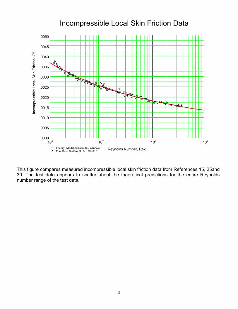
Incompressible Local Skin Friction Data

Theory: Modified Schultz / Grunow Test Data: Kulfan, R. M., D6-7161 Reynolds Number, Rex

Inco

mpr

essi

ble

Loca

l Ski

n Fr

ictio

n ,C

fi

106 107 108 109

.0050

.0045

.0040

.0035

.0030

.0025

.0020

.0015

.0010

.0005

.0000

This figure compares measured incompressible local skin friction data from References 15, 25and39. The test data appears to scatter about the theoretical predictions for the entire Reynoldsnumber range of the test data.

9

Page 10

106 107 108 109

Incompressible Local Skin Friction Data

[ ∆Cf = Cftest - Cftheory ] x 104

4

3

2

1

0

-1

-2

-3

-4

+1σMean-1σ

106 107 108 109Rex

+1σ

Mean

6543210-1-2-3-4-5-6

[ ∆Cf / Cftheory ] x 102

Rex

-1σ

Cf

106 107 108 109Rex

Theory: Modified Schultz / Grunow Test Data: Kulfan, R. M., D6-7161

.0050

.0045

.0040

.0035

.0030

.0025

.0020

.0015.

.0010

.0005

.0000

2.52.01.51.00.50.0

-0.5-1.0-1.5-2.0-2.5

[ ∆Cf = Cftest - Cftheory ] x 104

3.02.52.01.51.00.50.0

-0.5-1.0-1.5-2.0-2.5-3.0

[ ∆Cf / Cftheory ] x 102

Rmserror

meanabs.error

Mean Mean

+1σ

+1σ

-1σ

-1σ

meanabs.error

Rmserror

Statistical analysis of the differences between the test data and corresponding Cf predictionsshows that the mean of the differences is ∆Cf = -.000000671 which corresponds to an averagedifference of 0.13% .The standard deviation of data about the mean is approximately 0.7counts of drag ( ∆Cf = 0.000067) which corresponds to 2.8% of the corresponding predictedvalue. The constant 0.288 in the original Shultz / Grunow equation would result in a mean differencebetween the test and theory of - 2.6% The modified Shultz / Grunow equation therefore appears to provide an accurate estimate ofincompressible local skin friction coefficient over the entire range of Reynolds Numberscovered by the test data.

10

Page 11

Prediction of Compressibility Effects on Skin Friction• Monaghan Mean Enthalpy Method

Cf/C

fi

CF/

CFi

0 1 2 3 4 5 6 7 8 9 100

0.05

0.1

0.15

0.2

0.25

0.3

0.35

0.4

0.45

0.5

0.55

0.6

0.65

0.7

0.75

0.8

0.85

0.9

0.95

1

Theory: Rex = 106

Theory: Rex = 107

Test Data: Kulfan, R. M. , D6-7161Test Data: White, F. M., "Viscous Fluid Flow"

This figure includes comparisons of the predicted effects of Mach number on the ratio ofcompressible skin friction to incompressible skin friction at the same Reynolds. The experimentaldata are from thirteen independent experiments. The sources of the test data are given inReferences 1 and 2. The test data correspond to Reynolds number between 106 and 107. Thetheoretical predictions shown in the figure were obtained using the Monaghan T* equation. Thepredictions appear to match the Mach number trends quite well.

11

Page 12

Compressibility Component Effects

• Monaghan Mean Enthalpy Method

Kinematic Viscosity Effect

Dynamic Pressure Effect

0 1 2 3 4 5 6 7 8 9 10

2.5

2.0

1.5

1.0

0.5

0.0

Loca

l Ski

n Fr

ictio

n R

atio

Cf/

Cfi

Mach NumberKinematic Viscosity + "q" EffectKinematic Viscosity EffectTest Data: Kulfan, R. M., D6-7161Test Data: White, F. M., "Viscous Fluid Flow"Reference

This figure shows the elements of the compressibility corrections. The referencetemperature reduces the kinematic viscosity and therefore decreases the effectiveReynolds number. This increases the effective skin friction coefficient. The dynamicpressure effect associated with reduction in effective density overpowers the kinematicviscosity and results in the reduced skin friction coefficient when corrected back to freestream reference conditions.

12

Page 13

Comparison of Compressibility Effects Predictions

0 1 2 3 4 5 6 7 8 9 10

1.00

0.90

0.80

0.70

0.60

0.50

0.40

0.30

0.20

0.10

0.00

Mach Number

Skin Friction Ratio Cf / Cfi CF/CFiSk

in F

rictio

n R

atio

Cf/

Cfi

C

F/C

Fi

Theory: Monaghan Rex = 5x106

Theory: Sommer / Short Rex = 5x106

Test Data: Kulfan, R. M. D6-7161Test Data: White, F. M. , "Viscous Fluid Flow"

This compares the compressible skin friction predictions obtained using the Monaghan T* equationwith the predictions obtained using the Sommer-Short T* equation. The Sommer-Short T* equation results in compressible skin friction values consistently higher thanpredicted using the Monaghan method. It was for this reason that the Boeing US SST programswitched from the Monaghan method to the Sommer-Short method. The full scale SST performance predictions were obtained from wind tunnel data corrected to full scaleconditions. Wind tunnel skin friction drag is higher than the full scale conditions. Using higher skinfriction values calculated by the Sommer -Short method resulted larger skin friction corrections. Thisresulted in higher L/D assessments for the SST.

13

Page 14

Monagham Sommer and Short

[ ] [ ]∆ CfCfi

CfCfi

CfCfiTHEORY TEST

= − [ ] [ ]∆ CfCfi

CfCfi

CfCfiTHEORY TEST

= − [ ] [ ]∆ CfCfi

CfCfi

CfCfiTHEORY TEST

= −

∆ CfCfi

CfCfi

∗102

.04

.03

.02

.01

.00-.01-.02-.03-.04

.04

.03

.02

.01

.00-.01-.02-.03-.04

.04

.03

.02

.01

.00-.01-.02-.03-.04

6.0

4.0

2.0

0.0

-2.0

-4.0

-6.0

% %%6.0

4.0

2.0

0.0

-2.0

-4.0

-6.0

6.0

4.0

2.0

0.0

-2.0

-4.0

-6.0

Kulfan

T*/T1 =1 + 0.1246 M12 T*/T1 =1 + 0.1151 M1

2 T*/T1 =1 + 0.1198 M12

Evaluation of Reference Temperature Equations

Mean

+1σ

-1σ

meanabs.error

Rmserror

Mean

Mean

Mean

MeanMean

meanabs.error

meanabs.error

meanabs.error

meanabs.error

meanabs.error

Rmserror

Rmserror

Rmserror

Rmserror

Rmserror

+1σ

+1s

+1σ

+1σ

+1σ

-1σ

-1σ

-1σ

-1σ

-1σ

∆ CfCfi

CfCfi

∗102

∆ CfCfi

CfCfi

∗102

Statistical analyses of the differences between Cf predictions and the corresponding test data areshown in this figure. The theoretical predictions were obtained using three different T* equations. The “scatter” in the test - theory increments are essentially equal. The mean of the differencesbetween the test and theory, however differs between the predictions obtained using the different T*equations. The “mean” of the theory - test differences obtained using the Monaghan T* equation is approximately1% low. The “mean” of the theory - test differences obtained using the Sommer-Short T* equation isapproximately 1% high. The constant for the Kulfan T* equation was therefor chosen to be theaverage of the Sommer-Short and the Monaghan constants. This essentially resulted in a mean error between the test data and the theoretical predictions of zero. The test data scatter about the mean has a standard deviation of about 4.5%. This large scatter is inpart due to the variations of Reynolds number of the test data. The Reynolds number for the test data106 to 107

14

Page 15

.0050

.0045

.0040

.0035

.0030

.0025

.0020

.0015

.0010

.0005

.0000106 107 108Rex

Reynolds Number

Cf

Mach = 0.0

Mach = 2.0Mach = 2.95

Conversion of Compressible Cf Data to Equivalent Incompressible (Cfi)eq Data

Theory

X

Mach 0.20 Matting, F. W., et alMach 2.00 Shutts, W. H., et alMach 2.95 Matting, F. W., et al

• Kulfan T* Equation• Modified Schultz-Grunow Cf Equation

This figure contains comparisons of theoretical predictions of Cf with test data for three Machnumbers from 0.0 to approximately 3.0. The theory in this figure used the Kulfan T* equation.

15

Page 16

.0050

.0045

.0040

.0035

.0030

.0025

.0020

.0015

.0010

.0005

.0000106 107 108

Reynolds Number, Rex

Cf

• (Cfi)eq = (T*/T1) x Cf

• (Rex)eq = (Rex) x (T1/T* µ1/µ*)Mach = 0.0

Mach = 2.0Mach = 2.95

Conversion of Compressible Cf Data to Equivalent Incompressible (Cfi)eq Data

Theory

X

Mach 0.20 Matting, F. W., et alMach 2.00 Shutts, W. H., et alMach 2.95 Matting, F. W., et al

• Kulfan T* Method• Modified Schultz-Grunow Cf Equation

CfTT

xTT

= • • •

−

0 295 1 1

2 45

. log Re* * *

.µµ

Mach = 0.0

Mach = 2.95

.0050

.0045

.0040

.0035

.0030

.0025

.0020

.0015

.0010

.0005

.0000

Cf

106 107 108

Reynolds Number, Rex

νeffect

qeffect

In order to assess the accuracy of the Cf predictions to account for compressibility or Mach numbereffects, the test data were converted to equivalent incompressible values of Cfi and Reynoldsnumber. An example of this transformation is shown in the Figure. The Equivalent incompressible Reynolds number is less than the actual test Reynolds number. Theequivalent incompressible skin friction coefficient is higher than the actual measured skin frictioncoefficient. The Reynolds number correction has been calculated using the Sutherland viscosity equation. Theresulting equation is:

TT T

T

TT

1 1

1

2 51

1 198 7198 7* * * .

*..

µµ

=

++

The temperature in the above equation is in degrees Rankine. For the current study the local statictemperature was assumed to be 70 deg F. This corresponds to 529.6 deg R.

=

+=

1

*

1*

1 706.459

TTTT

T

16

Page 17

.0050

.0045

.0040

.0035

.0030

.0025

.0020

.0015

.0010

.0005

.0000

.0050

.0045

.0040

.0035

.0030

.0025

.0020

.0015

.0010

.0005

.0000106 107 108 106 107 108Rex

Reynolds Number(Rex)eq

Equivalent Incompressible Reynolds Number

Cf (Cfi)eq

• (Cfi)eq = (T*/T) x Cf

• (Rex)eq = (Rex) x (T/T* µ/µ*)

Mach = 0.0

Mach = 2.0

Mach = 2.95

Conversion of Compressible Cf Data to Equivalent Incompressible (Cfi)eq Data

Theory

X

Mach 0.20 Matting, F. W., et alMach 2.00 Shutts, W. H., et alMach 2.95 Matting, F. W., et al

• Kulfan T* Method• Modified Schultz-Grunow Cf Equation

This transformation procedure, as shown in the Figure, “collapses” all of the test data about theincompressible skin friction curve. This approach can provide a convenient means to assessthe accuracy of the theoretical methods to account for compressibility effects simultaneouslyover a range of Mach numbers and Reynolds numbers.

17

Page 18

Conversion of Compressible Cf Data to Equivalent Incompressible (Cfi)eq Data

.0050

.0045

.0040

.0035

.0030

.0025

.0020

.0015

.0010

.0005

.0000106 107 108

(Rex)eqEquivalent Incompressible Reynolds Number

(Cfi)eq

• (Cfi)eq = (T*/T) x Cf

• (Rex)eq = (Rex) x (T/T* µ/µ*)

• Kulfan T* Method• Modified Shultz-Grunow Cf Equation

Mach 1.70 Matting, F. W., et alMach 2.00 Shutts, W. H., et alMach 2.15 Shutts, W.H., et alMach 2.25 Shutts, W.H., et alMach 2.50 Shutts, W.H.; Coles, D.Mach 2.95 Matting, F. W., et al

+X

X

Cfi

Mean

+σ

-σ

Mean

+1σ

-1σmeanabs.error

Rmserror

[ ∆Cf / Cftheory ] x 102

+1σ

-1σ

Mean

meanabs.error

Rmserror

5.04.03.02.01.00.0

-1.0-2.0-3.0-4.0-5.0

2.52.01.51.00.50.0-0.5-1.0-1.5-2.0-2.5

Rmserror

meanabs.error

Mean+1σ

[ ∆Cf = Cftest - Cftheory ] x 104

-1σ

[ ∆Cf / Cftheory ] x 102

This shows transformed experimental data for six different sets of test data obtained at Mach numbersfrom 1.7 to 2.95. The incompressible Mach number data form the previous plot has not been includedin the above figure since it is desired to assess the ability of the different T* equations to account forMach number effects on skin friction. The figure includes the statistically determined differences between the transformed equivalentincompressible skin friction and the modified Shultz-Grunow theoretical Cf predictions. The Kulfan T*equation was used for the transformation process. The “mean” of the differences between thetransformed skin friction data and the incompressible Cf predictions is essentially. The “ scatter” of the test has a standard deviation of about 1 drag count ( ∆Cf ~ 0.0001). Thiscorresponds to about a 3.8% scatter of the test data about the theoretical Cf predictions over theentire Reynolds number range and Mach number conditions represented by the test data. The table below shows the results obtained different T* equations. On the average, the Monaghanpredictions tend to underestimate the test data by about 0.3 counts or 1.2 % and the Sommer-Shortpredictions are about 0.3 counts high corresponding to about 1.0%. The Kulfan T* method providesthe best estimate of the compressibility effects. The “scatter” in the compressible theoretical - experimental transformed skin friction increments areonly slightly higher than the scatter in the incompressible data shown in figure 10. ( 0.7 counts versus1 count). This is most likely because the transformation to equivalent Cfi amplifies the magnitude ofthe Cf values and hence the absolute differences.

Monaghan T* Eqn. Sommer-Short T* Eqn Kulfan T* Eqn.

∆Cf (counts)

∆Cf /Cf ( % )

∆Cf (counts)

∆Cf /Cf ( % )

∆Cf (counts)

∆Cf /Cf ( % )

Mean -.301 -1.2 .308 1.00 .00071 .085

σ 1.022 3.8 .985 3.0 1.066 4.0

18

Page 19

0 2 4 2.lo g (R e * )

C F ix C F i=

[ ]CFi x=−0 463 2 6. * log(Re ) .

Comparison of Incompressible Average Skin Friction Methods

Karmen - Schoenherr EquationModified Prandtl - Schlichting Equation

106 107 108 109

Reynolds Number, Rex

0.0050

0.0050

0.0030

0.0020

0.0010

0.0000

CFi

The most widely accepted in compressible local skin friction equation is the Karmen / Schoenherrequation: This is compared in this figure with the less sophisticated modified Prandtl / Schlichting equation. The modification was simply replacing the standard constant “0.460” by “0.463”. The meandifference between the CF values calculated by the Prandtl-Schlichting equation and by theKarmen-Schoenherr equation was -0.0000013 over the complete Reynolds number range. Thestandard deviation was calculated to be 0.00000678. Consequently, the simpler modified Prandtl-Schlichting equation was used in the current study. It is interesting that though out their technical careers. Prandtl and Von Karmen often tackled thesame fluid dynamic problem. Their results almost always differed in the analytical formulationsand the form of the equations describing the flow phenomena. Computed results were alwayswithin a few percent of each other.

)log(Re242.0 CFixCFi

⋅=

6.2))(Re(463.0 −⋅= xLogCfi

19

Page 20

Average Skin Friction Coefficient: Test vs Theory

Test Data: Kulfan, R. M., D6-7161

Mach = 2.5

Mach = 2.0

Mach = 0.0Mach = 1.61

.0050

.0045

.0040

.0035

.0030

.0025

.0020

.0015

.0010

.0005

.0000106 107 108

Reynolds Number, Rex

CF

• Kulfan T* Method• Modified Prandtl-Schlichting CF Equation

Comparisons between theoretical and experimental average skin friction data are shown in thefigure. The lack of additional test data is attributed to the difficulty in obtaining average skin frictiondata by direct force measurements. Most often, average skin friction data are obtained byapplication of the momentum integral equation to boundary layer velocity profile measurements.The uncertainties of the interference between the pitot probes used for the measurements and thesurface introduces errors that are difficult to correct. The data shown in the Figure for Mach 2.0 and Mach 2.5, were obtained from force measurementson the cylindrical portion of a cone-cylindrical body of revolution. The Mach 1.61 data wereobtained with an ogive - cylinder body of revolution. Three dimensional effects are considered tobe small on the cylindrical sections. However determining the “effective origin” for the flow over thecylindrical can certainly introduce substantial errors. The theoretical predictions match the Mach 2.0 and Mach 2.5 data quite well. Theory underestimated the friction drag at Mach 1.6. This is believed to be due to a bias in the test data. The results of the data correlations shown in this paper indicate that comparisons with local skinfriction data is the best approach to evaluate any methods for prediction of flat plate skin frictiondrag.

20

Page 21

Turbulent Boundary Layer

The Edge of a Turbulent Boundary Layer is Sharp But Very Irregular

In the current HSCT studies estimates of the boundary layer height are used to specify the height of theboundary layer diverter to keep the inlet from ingesting portions of the boundary layer. During the course of the investigation described in Reference 1, experimental measurements ofvelocity profiles were found. It was also then possible to study the growth characteristics of a turbulentboundary layer over a flat plate. A method was developed to predict the growth of a turbulent boundarylayer on a flat plate. This method has been revised in the current study. The edge of a turbulent boundary layer bounded by a free stream of negligible turbulence has a sharpbut very irregular outer limit as shown above. The velocity tends to approach the free stream velocityasymptotically. Hence the definition of the thickness of a turbulent boundary layer is subject to manyvariations. A common definition of the edge of the boundary layer, δ, is the height at which the velocityis equal to some percentage of the free stream value. Typically a value of 0.995 is used.

21

Page 22

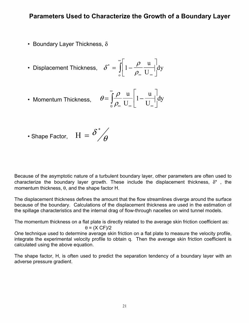
Parameters Used to Characterize the Growth of a Boundary Layer

• Boundary Layer Thickness, δ

• Momentum Thickness,

• Displacement Thickness,

• Shape Factor,

δρ

ρ* = −

∞ ∞

∞

∫ 1u

Udy

o

θρ

ρ= −

∞

∞

∞ ∞∫0

1u

Uu

Udy

H = δθ

*

Because of the asymptotic nature of a turbulent boundary layer, other parameters are often used tocharacterize the boundary layer growth. These include the displacement thickness, δ* , themomentum thickness, θ, and the shape factor H. The displacement thickness defines the amount that the flow streamlines diverge around the surfacebecause of the boundary. Calculations of the displacement thickness are used in the estimation ofthe spillage characteristics and the internal drag of flow-through nacelles on wind tunnel models. The momentum thickness on a flat plate is directly related to the average skin friction coefficient as: θ = (X CF)/2 One technique used to determine average skin friction on a flat plate to measure the velocity profile,integrate the experimental velocity profile to obtain q. Then the average skin friction coefficient iscalculated using the above equation. The shape factor, H, is often used to predict the separation tendency of a boundary layer with anadverse pressure gradient.

22

Page 23

Calculation Of Boundary Layer Characteristics

1. Approximate Velocity Profile as:

2. Determine “N” Experimentally

3. Calculate δ* From :

4. Calculate δ From : and

uU

y N

∞=

δ

1

δ θ

θ

* = ∗ ∗

=•

HHH

X CF

ii

2

δδ

ρρ δ δ

*

= −

∞∫ 1

1

0

1 yd

yN δδδδ

=

*

*

Often in boundary layer studies, it is convenient to represent the velocity profile by a power lawrelation of the form: This approximate form of the turbulent boundary velocity profile has been used to develop a four stepprocess for predicting the boundary layer thickness. The boundary layer thickness is defined as theheight at which the velocity is essentially equal to the free stream velocity. The elements incorporated in the process for calculating the boundary layer thickness aresummarized above, and will be discussed in greater detail in subsequent figures.

NyUu

1

=

∞ δ

23

Page 24

.01 .02 .03 .04 .05 .06 .08 .1 .2 .3 .4 .5 .6 .7 .8 1.0.50

1.0

.90

.80

.70

.60

Height Above Surface, Y Inches

Velo

city

Rat

io,

u/ U

o

Experimental and Approximate Velocity Profile

Lower Guide

Approximate “1/N” Profile: N=6.75

Upper Guide

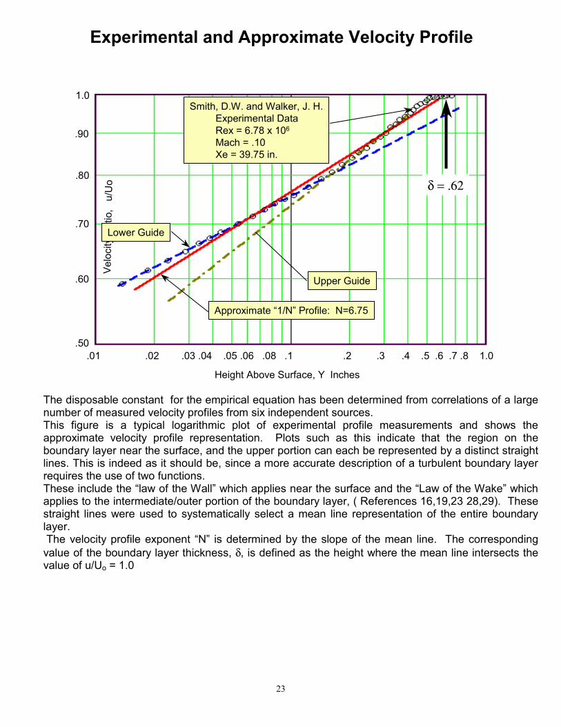
Smith, D.W. and Walker, J. H.Experimental DataRex = 6.78 x 106

Mach = .10Xe = 39.75 in.

δ = .62

The disposable constant for the empirical equation has been determined from correlations of a largenumber of measured velocity profiles from six independent sources. This figure is a typical logarithmic plot of experimental profile measurements and shows theapproximate velocity profile representation. Plots such as this indicate that the region on theboundary layer near the surface, and the upper portion can each be represented by a distinct straightlines. This is indeed as it should be, since a more accurate description of a turbulent boundary layerrequires the use of two functions. These include the “law of the Wall” which applies near the surface and the “Law of the Wake” whichapplies to the intermediate/outer portion of the boundary layer, ( References 16,19,23 28,29). Thesestraight lines were used to systematically select a mean line representation of the entire boundarylayer. The velocity profile exponent “N” is determined by the slope of the mean line. The corresponding

value of the boundary layer thickness, δ, is defined as the height where the mean line intersects thevalue of u/Uo = 1.0

24

Page 25

0.4 0.45 0.5 0.55 0.6 0.65 0.7 0.75 0.8 0.85 0.9 0.95 10

0.05

0.1

0.15

0.2

0.25

0.3

0.35

0.4

0.45

0.5

0.55

0.6

0.65

0.7

Lower GuideUpper Guide" 1/N" ProfileTest Data

Velocity Ratio, u/Uo

Hei

ght A

bove

Sur

face

, Y

in

ches

Experimental and Approximate Velocity Profiles

δδδδ = 0.62

uU o

y N=

δ

1

Lower Guide

Upper Guide

This is a conventional plot of the velocity profile data shown in the previous chart. The various boundary layer growth characteristics were calculated from the measured velocity profiledata and also using the approximate “power law” velocity profile. The results are summarized in thetable below. The approximate velocity profile “matched” to fit the experimental velocity profile by the processdescribed on the previous page, does provides a good approximation to the turbulent boundary layergrowth characteristics.

Measured Profile

Approximate Profile

“Error” %

δ* 0.0803 0.0801 -0.25

θ 0.0592 0.0613 3.5

H 1.357 1.307 -3.7

25

Page 26

1 106 1 107 1 1080

1

2

3

4

5

6

7

8

9

10

Analytic RepresentationSigalla, A.Kleebanoff, P. S., Diehl, Z. W.Smith, D. W., Walker, J.H.

Reynolds Number, Rex

Vel

ocity

Pro

file

"N"

Fact

or

Incompressible Velocity Profile “N” Factoru/Uo = (y/δδδδ)1/N

( )N

CfiCfi

=− ∗

max

. ( ),

.

.

0 1035 26

0 75

0 75

Incompressible velocity profile data from a number of independent sources were used to determine“appropriate” values of N to represent a turbulent boundary layer. The results as shown in thisfigure, indicate that the value of “N” is strongly dependent on Reynolds number. The equation shown in the figure was developed in the current study to represent the effect ofReynolds number on “N” as determined from the experimental data.

26

Page 27

1 106 1 107 1 1080

1

2

3

4

5

6

7

8

9

10

Analytic RepresentationShutts, W.H., et al : Mach = 1.5 to 2.5Matting, F.W., et al : Mach = 2.95 to 4.2

Reynolds Number, Rex

Vel

ocity

Pro

file

"N"

Fact

or

Supersonic Velocity Profile “N” Factoru/Uo = (y/δδδδ)1/N

( )N

CfiCfi

=− ∗

max

. ( ),

.

.

0 1035 26

0 75

0 75

The data in this figure are values of “N” determined from compressible boundary layer measurements for a number of Mach numbers from 1.5 to 4.2. The compressible values of “N” appear to scatter about the empirical equation that was developed from the incompressible velocity profile data. Thus is appears that the shape of a turbulent depends on Reynolds number but is independent of Mach number. This result should not be surprising for it is implied by the concept of the reference temperature approach to calculate supersonic skin friction drag. Skin friction depends on the shape of the boundary layer as well as the density and viscosity in the boundary. The reference temperature method as defined earlier in this note assumes that compressibility only changes the effective values if density and viscosity. Hence, Mach number doesn’t change the velocity profile shape. Developing an analytic expression for “N” was the second step in the process for developing a method to predict the boundary layer thickness.

27

Page 28

Theory

Ashkenas, H., and Ridell, F. R.Sigalla, A.Klebanoff, P. S.Smith, D. W., and Walker, J. H.

Reynolds Number, Rex

Inco

mpr

essi

ble

Shap

e Fa

ctor

, H

i

Incompressible Shape Factor Data

H iC fi

=−

11 4 7 5. *

105 106 107 108

2.0

1.8

1.6

1.4

1.2

1.0

0.8

0.6

0.4

0.2

0.0

Coles analytic results

In incompressible flow the boundary layer displacement thickness and momentum thicknessequations are: In incompressible flow, the value of H for a flat plate turbulent flow is a unique function of the“shape” of the boundary layer. In principal, the variation of H with Reynolds number could be determined from the approximatevelocity profile shape and the empirical equation for “N”. As previously shown, the approximatevelocity profile shape provides a very good estimate for δ* . The values for both θ and Hcalculated using the approximate velocity profile are not as accurate. Consequently, it wasdecided to use an equation for H developed by Clauser (presented in Ref 28) based on a moresophisticated representation of the boundary layer based on the “velocity defect” concept.Experimental values of the incompressible shape factor, Hi, are compared with a modified versionof Clauser’s equation in which the constant 4.75 replaced Clauser’s original value of 4.31. Also shown in the figure are analytic values for Hi calculated by Coles (presented in Ref 35) using“log” wall relations for the boundary layer.

dyUu

o∫∞

∞

−= 1*δ

dyUu

Uu

−=

∞

∞

∞∫ 10

θ

θδ *

=H

28

Page 29

Mach Number Effect on Boundary Layer Shape FactorReynolds Number = 4x106 to 30x106

Rubesin, M. W., et al

TheoryShutts, W. H., et al

Mach Number

Shap

e Fa

ctor

Rat

io,

H/H

i

H/Hi = 1+r(γ-1)Mo2

0.0 0.2 0.4 0.6 0.8 1.0 1.2 1.4 1.6 1.8 2.0 2.2 2.4 2.6 2.8 3.0

5.04.84.64.44.24.03.83.63.43.23.02.82.62.22.01.81.61.41.21.00.80.60.40.20.0

Following Monaghan (Ref 27), the shape factor for the turbulent boundary layer on a flat plate can be related to theincompressible value Hi, the free stream temperature T∞, the wall temperature Tw, and the recovery temperature Tr, bythe equation: For an insulated surface this equation becomes: Experimental data shown in the figure appears to validate this equation. Hence, the shape factor for fully turbulent flatplate flow can be can be calculated as the product of two factor. One factor depends only on Reynolds number and thesecond factor depends only on Mach number. The equation implies that boundary layer displacement effects become much larger than the momentum thickness asMach number increases.

−+

−+=

∞∞

111TT

TT

HiH rw

( ) 211 ∞−+= MrHiH γ

29

Page 30

1 106 1 107 1 1080

0.10.20.30.40.50.60.70.80.9

11.11.21.31.41.51.61.71.81.9

22.12.2

Theory : Kulfan, R. M.Smith, D.W., and Walker, J.H. : Mach = 0.0 to 0.32

INCOMPRESSIBLE BOUNDARY LAYER THICKNESS

Reynolds Number, Rex

Bou

ndar

y La

yer T

hick

ness

, d/x

(%

)

We now have developed all the ingredients to calculate the boundary layer thickness for fully turbulentflat plate flow using the process shown in figure 23. Calculations of the variation of incompressible flat plate boundary layer thickness are compared withtest data from reference 1. The theoretical predictions obtained using this process closely matches thetest data.

30

Page 31

Incompressible Boundary Layer Displacement Thickness

0.4

0.3

0.2

0.1

0.0

δ*/x %

106 107 108Reynolds Number, Rex

Theory

Test

Smith, D. W., and Walker, J.H.: Mach = 0.0 to 0.32Theory: Kulfan, R. M.

The boundary layer displacement thickness can be calculated by the shape factor equations and theaverage flat plate skin friction coefficient as: Predictions of incompressible displacement thickness are compared with test data in the figure. Theagreement between the theory and the test data is quite good.

CFHiHHi

X 2

*

=δ

31

Page 32

106 107

108

Reynolds Number

106 107 108

Reynolds Number

Boundary Layer Thicknessδδδδ / X x100

Boundary Layer Displacement Thicknessδδδδ* / X x100

Mach = 0.0Mach = 1.0Mach = 2.0Mach = 3.0

2.2

2.0

1.8

1.6

1.4

1.2

1.0

0.8

0.6

0.4

0.2

0.0

1.0

0.9

0.8

0.7

0.6

0.5

0.4

0.3

0.2

0.1

0.0

Compressibility Effects on Boundary Layer Thickness

Theory: Kulfan, R.M.

Increasing Mach No.

Increasing Mach No.

Boundary layer thickness and displacement thickness have been calculated for a range of Reynoldsnumbers and Mach numbers from 0 to 3 using the methods presented in this paper. The overall boundary layer thickness is seen to be relatively insensitive to Mach number. Theboundary layer displacement thickness, however, grows rapidly as Mach number increases.

32

Page 33

TheoryMach = 1.7

TestM = 1.6 to 1.8

TheoryMach = 3.0 Theory

Mach = 0.0

TheoryMach = 2.0

TestM = 1.6 to 3.0

TestM = 0.0 to .32Test

M = 2.95

TestM = 2.0 to 2.2

TheoryMach = 3.0

Compressibility Effects on Boundary Layer Thickness2.42.22.01.81.61.41.21.00.80.60.40.20.0

2.42.22.01.81.61.41.21.00.80.60.40.20.0

δ/x %

δ/x %

δ/x %

δ/x %2.42.22.01.81.61.41.21.00.80.60.40.20.0

2.42.22.01.81.61.41.21.00.80.60.40.20.0

106 107 108Rex 106 107 108Rex

106 107 108Rex 106 107 108Rex

Shutts, W. H. et al

Matting, F. W. et al

Shutts, W. H. et al

Compressible boundary layer thickness predictions are compared with test data in this Figure forMach numbers of 1.7, 2.0 and 3.0. Although there is quite a bit of data scatter, the data appears tovalidate the boundary layer thickness predictions. The fourth figure contains the incompressible data from the previous figure and the three sets ofcompressible data. This appears to substantiate the conclusion that the thickness of a turbulentboundary layer is indeed relatively insensitive to Mach number.

33

Page 34

Conclusions• Modified Incompressible Equations and Improved T*/T Method Predict “Mean” of Available Flat Plate Skin Friction Drag Measurements

• New Methods Presented That Appear to Provide Good Estimates of Boundary layer Thickness and Displacement Thickness

• Compressibility Effects Have Very Little Effect on The Shape or Heightof the Turbulent Flat Plate Velocity Profile.

• Boundary Layer Displacement Thickness Increases Rapidly With Mach Number

• Comparisons of Navier Stokes CFD Predictions of Flat Plate Turbulent Skin Friction Drag and Boundary Layer Growth, With the Test Data and / or Theory Presented in This paper, is considered to be a Necessary and Vital Step to Validating the Codes For HSCT Viscous Drag Predictions .

• Need Additional / Quality Experimental CF Data:- Locate Available Existing Data - Symmetric Model Tests - Segmented Axisymmetry Body of Revolution - Utilize TU-144 Flight Test Data- ???

The modified incompressible CF equations and the improved T* equation presented in the paperappear to consistently match the test better than the other flat plate CF methods currently in use onthe HSCT program. It is recommended that the methods presented here, be adapted as the officialHSCT flat plate calculation methods. The boundary layer thickness, and displacement thickness calculations methods presented in thispaper seem to be validated by the existing data. Compressibility effects have little effect on either the shape or height of a turbulent boundary layer.The displacement thickness however varies rapidly with increasing Mach number. Comparisons of Navier-Stokes predictions, of the skin friction drag and boundary layer growthcharacteristics for fully turbulent flat plate flow, with the theory and/or test data presented in thispaper is considered to be a necessary and vital step in validation of the CFD codes for HSCTviscous drag predictions. This is just the first step in the total validation process that may alsoinclude comparisons with data from tests of a symmetric HSCT type configuration, or data fromtests of a long segmented cone/cylinder body, and utilization of the newly acquired TU-144 flighttest data

34

REFERENCES Each reference listed below contains one or more of the following criteria (as denoted by the letter inthe brackets): A. Extensive experimental measurement and data reduction techniques. B. Presentation or discussion of analytical techniques. C. Experimental data. D. Extensive bibliography. 1. Kulfan, Robert M., "Turbulent Boundary Layer Flow Past a Smooth Adiabatic Flat Plate",

Boeing Document D6-7161, May 1961 [B,C,D] 2. White, Frank M. VISCOUS FLUID FLOW, Mc Graw - Hill Book Company, 1974, [ B,C,D] 3. Wegener, Winkler, Sibulkin. "A Measurement of Turbulent Boundary Layer Profiles and Heat

Transfer Coefficients at Mach 7.0", Journal of Aero-nautical Sciences, Vol.20, No.3, 1953.[A,C]

4. Chapman and Kester. "Measurement of Turbulent Skin Friction on Cylinders in Axial Flow at

Subsonic and Supersonic Velocities," Journal of Aeronautical Sciences, Vol.20, No.7, 1953.[A,B,C,D]

5. Chapman and Kester. 11Turbulent Boundary Layer and Skin Friction Measurements in Axial

Flow along Cylinders at Mach Numbers between 0.5 and 3.6." NACA TN 3097. [A,B,C,D] 6. Naleid, J. F. "Experimental Investigation of the Impact Probe Method of Measuring Local Skin

Friction at Supersonic Speeds in the Presence of an Adverse Pressure Gradient." DefenseResearch Laboratory Report. D.R.L. - 432, CF - 273. [A,C]

7. Sibulkin, M. "Boundary Layer Measurements at Supersonic Nozzle Throats." Journal of

Aeronautical Sciences, April, 1957. [A,C] 8. Winkler, E. M., Cha, M. H. "Experimental Investigations of the Effect of Heat Transfer on

Hypersonic Turbulent Boundary Layer Skin Friction." Journal of Aero/Space Sciences,February, 1959. [A,C]

9. Shutts, W. H., Hartwig, W. H., and Weiler, J. E. "Final Report on Turbulent Boundary Layer

and Skin Friction Measurements on a Smooth, Thermally Insulated Flat Plate at SupersonicSpeeds." Defense Research Laboratory Report. D.R.L. - 364, C.M. - 823. [A,C,D]

10. Coles, Donald. "Measurements of Turbulent Friction on a Smooth Flat Plate in Supersonic

Flow." Journal of Aeronautical Sciences, Vol.21, No.7, July, 1954. [A,C] 11. Korkegi, Robert H. "Transition Studies and Skin Friction Measurements on an Insulated Flat

Plate at a Mach Number of 5.8." Journal of Aeronautical Sciences, Vol.25, No.2, February,1956. [A,C]

35

REFERENCES (Continued) 12. Sommer, Simon C., and Short, Barbara J. "Free Flight Measurements of Skin Friction of

Turbulent Boundary Layer Skin Friction in the Presence of Severe Aerodynamic Heating atMach Numbers from 2.8 to 7.0." NACA TN 3391, March, 1955. [A,B,C]

13. Sommer, Simon C., Short, Barbara J. "Free Flight Measurements of Skin Friction of Turbulent

Boundary Layers with High Rates of Heat Transfer at Supersonic Speeds." Journal ofAeronautical Sciences, June, 1956. [A,B,C]

14. Rubesin, M. W., Maydew, R. C., and Varga, S. A. "An Analytical and Experimental Investigation

of Skin Friction of the Turbulent Boundary Layer on a Flat Plate at Supersonic Speeds." NACATN 2305, February, 1951. [A,B,C]

15. Matting, F. We, Chapman, D. R., Nyholm, J. R., Thomas, A. G. "Turbulent Skin Friction at High

Mach Numbers and Reynolds Numbers." PROCEEDINGS OF THE 1959 HEAT TRANSFERAND FLUID MECHANICS INSTITUTE. Stanford University Press, 1959. [A,B,C,D]

16. Dhawan, Satish. "Direct Measurements of Skin Friction." NACA Report 1121, 1953. [A,B,C,D] 17. Czarnecki, K. R., Sevier, J. R., and Carmel, N. M. "Effects of Fabrication 'type Roughness on

Turbulent Skin Friction at Supersonic Speeds." NACA TN 4299. [A,C] 18. Fenter, F. W., and Stalmach, C. J., Jr. "The Measurement of Local Turbulent Skin Friction at

Supersonic Speeds by Means of Surface Impact Pressure Probes." Defense ResearchLaboratory Report. D.R.L. - 392, CM - 878, October, 1957. [A,B,C,D]

19. Kuethe, A.M., and Schetzer,J. D. , FOUNDATIONS OF AERODYNAMICS John Wiley and

Sons, Incorporated, . New York, 1959. [B] 20. Nielsen, J. N. MISSILE AERODYNAMICS. New York, McGraw-Hill Book Company Inc., 1960.

[B,C] 21. Liepmann H. W., and Roshko, A., ELEMENTS OF GASDYNAMICS, John Wiley and Sons, Inc.,

New York 1957. [B,D] 22. Shapiro, A. H. THE DYNAMICS AND THERMODYNAMICS OF COMPRESSIBLE Flow. Vol.11,

New York, The Ronald Press Company, 1954. [B,C] 23. Schlichting, H. BOUNDARY LAYER THEORY. New York, Pergamon Press, 1955. [B,D] 24. Hilsenrathb J. et al. TABLES OF THERMAL PROPERTIES OF GASES. National Bureau of

Standards Circular 564, November, 1955. 25. Smith, D. W., and Walker, J. H. "Skin Friction Measurements in Incompressible Flow." NACA

TN 4231, 1958. [A,C]

36

REFERENCES (Continued) 26. Matting, F. W., Chapman, D. R., Nyholm, J. R., Thomas, A. G. "Turbulent Skin Friction at High

Mach Numbers and Reynolds Numbers in Air and Helium." NASA R-82. [A,B,C,D] 27. Monaghan, R. J. "On the Behavior of Boundary Layers at Supersonic Speeds." I.A.S. - R A. S

Proceedings, 1955. [B,D] 28. Lin, C. C. TURBULENT FLOWS AND HEAT TRANSFER. Vol.5, Princeton Series on High Speed

Aerodynamics and Jet Propulsion. Princeton University press, 1959. [B,D] 29. Thwaites, B. "Incompressible Aerodynamics." Oxford at the Claredon Press, 1960. [B,D] 30. KIebanoff, P.S., and Diehl, Z. E. "Some Features of Artificially Thickened Fully Developed

Boundary Layers with Zero Pressure Gradient." NACA Report 1110, 1952. [A,C,D] 31. Simon, P. C. and Kowalski, K. L. "Charts of Boundary Layer Mass Flow and Momentum for Inlet

Performance Analysis Mach Number Range, 0.2 to 5.0." NACA TN 3583, November, 1955. [B] 32. Ashkenas, H., and Riddell, F. R. "Investigation of the Turbulent Boundary Layer on a Yawed Flat

Plate." NACA TN 3383, 1955. [A,B,C] 33. KIebanoff, P.S. "Characteristics of Turbulence in a Boundary Layer with Zero Pressure Gradient."

NACA Report 1247, 1955. [A,B,C) 34. Sigalla, A. "Experiments with Pitot Tubes for Skin Friction Measurements." British ..Iron and Steel

Research Association Report P/2/58, List 92, 1958. [A,C] 35. Duncan, W. J., Thom, A. S.,Young, A. D., MECHANICS OF FLUIDS, American Elsevier

Publishing Co. New York, 1970. [A,B,C,D] 36. 36. Erickson, W. D. "Real-Gas Correction Factors for Hypersonic Flow Parameters in Helium."

NASA TN D-462, September, 1960. 37. Eckert, E. R. G. et al: "Prandtl Number, Thermal Conductivity, and Viscosity of Air-Helium

Mixtures." NASA TN D-533, September, 1960. 38. 38. Czarnecki, K. R. et al: "Investigation of Distributed Surface Roughness on a Body of

Revolutions at a Mach Number of 1.61." NACA TN 3230, June, 1954. [A,C] 39. 39. Smith, D. W., and Walker, J. H. "Skin Friction Measurements in Incompressible Flow." NACA

TR R-26, 1959. [A,C,D] 40. Eckert, Z. R. G. "Simplified treatment of the Turbulent Boundary Layer along a Cylinder in

Compressible Flow." Journal of Aeronautical Sciences, January, 1952. [B]