History-Dependent Risk Attitude * David Dillenberger † University of Pennsylvania Kareen Rozen ‡ Yale University June 2014 Abstract We propose a model of history-dependent risk attitude, allowing a decision maker’s risk attitude to be affected by his history of disappointments and elations. The decision maker re- cursively evaluates compound risks, classifying realizations as disappointing or elating using a threshold rule. We establish equivalence between the model and two cognitive biases: risk attitudes are reinforced by experiences (one is more risk averse after disappointment than after elation) and there is a primacy effect (early outcomes have the greatest impact on risk attitude). In a dynamic asset pricing problem, the model yields volatile, path-dependent prices. Keywords: history-dependent risk attitude, reinforcement effect, primacy effect, dynamic ref- erence dependence JEL Codes: D03, D81, D91 * This paper generalizes a previous version that circulated under the title “Disappointment Cycles.” We benefitted from comments and suggestions by Simone Cerreia-Vioglio, Wolfgang Pesendorfer, Ben Polak, Andrew Postlewaite, Larry Samuelson, and several seminar audiences. We thank Xiaosheng Mu for excellent research assistance. † Department of Economics, 160 McNeil Building, 3718 Locust Walk, Philadelphia, Pennsylvania 19104-6297. E-mail: [email protected]‡ Department of Economics and the Cowles Foundation for Research in Economics, 30 Hillhouse Avenue, New Haven, Connecticut 06511. E-mail: [email protected]. I thank the NSF for generous financial support through grant SES-0919955, and the economics departments of Columbia and NYU for their hospitality.
Transcript
History-Dependent Risk Attitude∗
David Dillenberger†
University of Pennsylvania
Kareen Rozen‡
Yale University
June 2014
Abstract
We propose a model of history-dependent risk attitude, allowing a decision maker’s riskattitude to be affected by his history of disappointments and elations. The decision maker re-cursively evaluates compound risks, classifying realizations as disappointing or elating usinga threshold rule. We establish equivalence between the model and two cognitive biases: riskattitudes are reinforced by experiences (one is more risk averse after disappointment than afterelation) and there is a primacy effect (early outcomes have the greatest impact on risk attitude).In a dynamic asset pricing problem, the model yields volatile, path-dependent prices.
∗This paper generalizes a previous version that circulated under the title “Disappointment Cycles.” We benefittedfrom comments and suggestions by Simone Cerreia-Vioglio, Wolfgang Pesendorfer, Ben Polak, Andrew Postlewaite,Larry Samuelson, and several seminar audiences. We thank Xiaosheng Mu for excellent research assistance.
‡Department of Economics and the Cowles Foundation for Research in Economics, 30 Hillhouse Avenue, NewHaven, Connecticut 06511. E-mail: [email protected]. I thank the NSF for generous financial support throughgrant SES-0919955, and the economics departments of Columbia and NYU for their hospitality.
Once bitten, twice shy. — Proverb
1 Introduction
Theories of decision making under risk typically assume that risk preferences are stable. Evidencesuggests, however, that risk preferences may vary with personal experiences. It has been shownthat emotions, which may be caused by exogenous factors or by the outcomes of past choices, playa large role in the decision to bear risk. Moreover, individuals are affected by unrealized outcomes,a phenomenon known in the psychological literature as counterfactual thinking.1
Empirical work has found evidence of history-dependent risk aversion in a variety of fields.Pointing to adverse consequences for investment and the possibility of poverty traps, developmenteconomists have observed a long-lasting increase in risk aversion after natural disasters (Cameronand Shah, 2010) and, studying the dynamics of farming decisions in an experimental setting, in-creases of risk aversion after failures (Yesuf and Bluffstone, 2009). Malmendier and Nagel (2011)study how personal experiences of macroeconomic shocks affect financial risk-taking. Controllingfor wealth, income, age, and year effects, they find that for up to three decades later, “householdswith higher experienced stock market returns express a higher willingness to take financial risk,participate more in the stock market, and conditional on participating, invest more of their liquidassets in stocks.” Applied work also demonstrates that changing risk aversion helps explain sev-eral economic phenomena. Barberis, Huang and Santos (2001) allow risk aversion to decreasewith prior stock market gains (and increase with losses), and show that their model is consistentwith the well-documented equity premium and excess volatility puzzles. Gordon and St-Amour(2000) study bull and bear markets, allowing risk attitudes to vary stochastically by introducing astate-dependent CRRA parameter in a discounted utility model. They show that countercyclicalrisk aversion best explains the cyclical nature of equity prices, suggesting that “future work shouldaddress the issue of determining the factors that underline the movements in risk preferences”which they identified.
In this work, we propose a model under which such shifts in risk preferences may arise. Ourmodel of history-dependent risk attitude (HDRA) allows the way that risk unfolds over time to af-fect attitude towards further risk. We derive predictions for the comparative statics of risk aversion.In particular, our model predicts that one becomes more risk averse after a negative experiencethan after a positive one, and that sequencing matters: the earlier one is disappointed, the more riskaverse one becomes.
1On the effect of emotions, see Knutson and Greer (2008) and Kuhnen and Knutson (2011), as well as Section 1.1.Roese and Olson (1995) offers a comprehensive overview of the counterfactual thinking literature.
1
To ease exposition, we begin by describing our HDRA model in the simple setting of T -stage,compound lotteries (the model is later extended to stochastic decision problems, in which the DMmay take intermediate actions). A realization of a compound lottery is another compound lottery,which is one stage shorter. The DM categorizes each realization of a compound lottery as anelating or disappointing outcome. At each stage, his history is the preceding sequence of elationsand disappointments. Each history h corresponds to a preference relation over one-stage lotteries.We consider one-stage preferences that are rankable in terms of their risk aversion. For example,an admissible collection could be a class of expected utility preferences with the Bernoulli functionu(x) = x1−ρh
1−ρh, where the coefficient of relative risk aversion ρh is history dependent.
The HDRA model comprises two key structural features: (1) compound lotteries are evaluatedrecursively, and (2) the DM’s history assignment is internally consistent. More formally, startingat the final stage of the compound lottery and proceeding backwards, each one-stage lottery is re-placed with its appropriate, history-dependent certainty equivalent. At each step of this recursiveprocess, the DM is evaluating only one-stage lotteries, the outcomes of which are certainty equiv-alents of continuation lotteries. Recursive evaluation is a common feature of models, but by itselfhas no bite on how risk aversion changes. To determine which outcomes are elating and disap-pointing, the DM uses a threshold rule that assigns a number (a threshold level) to each one-stagelottery encountered in the recursive process. Internal consistency requires that if a sublottery isconsidered an elating (disappointing) outcome of its parent sublottery, then its certainty equivalentshould exceed (or fall below) the threshold level corresponding to its parent sublottery. Internalconsistency is thus a way to give intuitive meaning to the terms elation and disappointment. Com-bined with recursive evaluation, it imposes a fixed-point requirement on the assignment of historiesin a multi-stage setting.
Besides imposing internal consistency, we do not place any restriction on how risk aversionshould depend on the history. Nonetheless, we show that the HDRA model predicts two well-documented cognitive biases; and that these biases are sufficient conditions for an HDRA repre-sentation to exist. First, the DM’s risk attitudes are reinforced by prior experiences: he becomesless risk averse after positive experiences and more risk averse after negative ones. Second, the DMdisplays a primacy effect: his risk attitudes are disproportionately affected by early realizations. Inparticular, the earlier the DM is disappointed, the more risk averse he becomes. We discuss evi-dence for these predictions in Section 1.1 below. Our main result thus provides a link between thetwo structural assumptions of recursive evaluation and internal consistency, and the evolution ofrisk attitude as a function of (personal) experiences.
Our model and its main result are general, allowing a wide class of preferences to be used for
2
recursively evaluating lotteries, as well as a variety of threshold rules. The one-stage preferencesmay come from the betweenness class (Dekel, 1986; Chew, 1989), which includes expected util-ity. The DM’s threshold rule may be either endogenous (preference-based) or exogenous. In thepreference-based case, the DM’s threshold moves endogenously with his preference; he comparesthe certainty equivalent of a sublottery to the certainty equivalent of its parent. In the exogenouscase, the DM uses a rule that is independent of preferences but is a function of the lottery at hand;for example, an expectation-based rule that compares the certainty equivalent of a sublottery to hisexpected certainty equivalent. All of the components of the HDRA model – that is, the single-stagepreferences, threshold rule, and history assignment – can be elicited from choice behavior.
We show that the model and characterization result also readily extend to settings that allowfor intermediate actions. As an application, we study a multi-period asset pricing problem wherean HDRA decision maker (with CARA preferences) adjusts his asset holdings in each period af-ter observing past dividend realizations. We show that the model yields volatile, path-dependentprices. Past realizations of dividends affect subsequent prices, even though they are statisticallyindependent of future dividends and there are no income effects. For example, high dividendsbring about price increases, while a sequence of only low dividends leads to an equity premiumhigher than in the standard, history-independent CARA case. Since risk aversion is endogenouslyaffected by dividend realizations, the risk from holding an asset is magnified by expected futurevariation in the level of risk aversion. Hence the HDRA model introduces a channel of risk that isreflected in the greater volatility of asset prices. This is consistent with the observation of excessvolatility in equity prices, dating to Shiller (1981).
This paper is organized as follows. Section 1.1 surveys evidence for the reinforcement andprimacy effects. Section 1.2 discusses related literature. Section 2 introduces our model in the set-ting of compound lotteries (for notational simplicity, we extend the setting and results to stochasticdecision trees only in Section 6). Section 3 contains our main result, which characterizes how riskaversion evolves with elations and disappointments. Section 4 describes how the components ofthe model can be elicited from choice behavior. Section 5 discusses further implications of themodel. Section 6 generalizes the choice domain in the model to stochastic decision trees and stud-ies a three-period asset pricing problem. Section 7 concludes. All proofs appear in the appendix.
1.1 Evidence for the Reinforcement and Primacy Effects
Our main predictions, the reinforcement and primacy effects, are consistent with a body of evi-dence on risk-taking behavior. Thaler and Johnson (1990) find that individuals become more riskaverse after negative experiences and less risk averse after positive ones. Among contestants in the
3
game show “Deal or No Deal,” Post, van den Assem, Baltussen and Thaler (2008) find mixed evi-dence, suggesting that contestants are more willing to take risks after extreme realizations. Guiso,Sapienza and Zingales (2011) estimate a marked increase in risk aversion in a sample of Italianinvestors after the 2008 financial crisis; the certainty equivalent of a risky gamble drops from 4,000euros to 2,500, an increase in risk aversion which, as the authors show, cannot be due to changesin wealth, consumption habits, or background risk. In an experiment with financial professionals,Cohn, Engelmann, Fehr and Marechal (2013) find that subjects primed with a financial bust aresignificantly more risk averse than subjects primed with a boom. As discussed earlier, Malmendierand Nagel (2011) find that macroeconomic shocks lead to a long-lasting increase of risk aversion.Studying initial public offerings (IPOs), Kaustia and Knupfer (2008) identify pairs of “hot andcold” IPOs with close offer dates and follow the future subscription activities of investors whosefirst IPO subscription was in one of those two. They find that “twice as many investors participatein a subsequent offering if they first experience a hot offering rather than a cold offering.” Pointingto a primacy effect, they find that the initial outcome has a strong impact on subsequent offerings,and that “by the tenth offering, 65% of investors in the hot IPO group will have subscribed to an-other IPO, compared to only 39% in the cold IPO group.” Baird and Zelin (2000) study the impactof sequencing of positive and negative news in a company president’s letter. They find a primacyeffect, showing that information provided early in the letter has the strongest impact on evalua-tions of that company’s performance. In general, sequencing biases2 such as the primacy effectare robust and long-standing experimental phenomena (early literature includes Anderson (1965));and several empirical studies, including Guiso, Sapienza and Zingales (2004) and Alesina andFuchs-Schundeln (2007)), argue that early experiences may shape financial or cultural attitudes.
The biological basis of changes in risk aversion has been studied by neuroscientists. As sum-marized in Knutson and Greer (2008) and Kuhnen and Knutson (2011), neuroimaging studies haveshown that two parts of the brain, the nucleus accumbens and the anterior insula, play a large role inrisky decisions. The nucleus accumbens processes information on rewards, and is associated withpositive emotions and excitement; while the anterior insula processes information about losses,and is associated with negative emotions and anxiety. Controlling for wealth and information, ac-tivation of the nucleus accumbens (anterior insula) is associated with bearing greater (lesser) riskin investment decisions. Discussing feedback effects, Kuhnen and Knutson (2011) note that:
[. . .] activation in the nucleus accumbens increases when we learn that the outcomeof a past choice was better than expected (Delgado et al. (2000), Pessiglione et al.(2006)). Activation in the anterior insula increases when the outcome is worse than
2Another well-known sequencing bias is the recency effect, according to which more recent experiences have thestrongest effect. A recency effect on risk attitude is opposite to the prediction of our model.
4
expected (Seymour et al (2004), Pessiglione et al (2006)), and when actions not chosenhave larger payoffs than the chosen one.
In a neuroimaging study with 90 sequential investment decisions by subjects, these feedback effectsare shown to influence subsequent risk-taking behavior (Kuhnen and Knutson, 2011).
1.2 Relations to the literature
In many theories of choice over temporal lotteries, risk aversion can depend on the passage of time,wealth effects or habit formation in consumption; see Kreps and Porteus (1978), Segal (1990),Campbell and Cochrane (1999) and Rozen (2010), among others. We study how risk attitudes areaffected by the past, independently of such effects. In the HDRA model, risk attitudes depend on“what might have been.” Such counterfactual thinking means that our model relaxes consequential-ism (Machina, 1989; Hanany and Klibanoff, 2007), an assumption that is maintained by the papersabove. Our form of history-dependence is conceptually distinct from models where current andfuture beliefs affect current utility (that is, dependence of utility on “what might be” in the future).This literature includes, for instance, Caplin and Leahy (2001) and Koszegi and Rabin (2009).
Caplin and Leahy (2001) propose a two-period model where the prize space of a lottery isenriched to contain psychological states, and there is an (unspecified) mapping from physical lot-teries to mental states. Depending on how the second-period mental state is specified to depend onthe first, Caplin and Leahy’s model could explain various types of risk-taking behaviors in the firstperiod. While discussing the possibility of second-period disappointment, they do not address thequestion of history-dependence in choices. We conjecture that with additional periods and an ap-propriate specification of the mapping between mental states, one could replicate the predictions ofour model. Koszegi and Rabin (2009) propose a utility function over T -period risky consumptionstreams. In their model, period utility is the sum of current consumption utility and the expectationof a gain-loss utility function, over all percentiles, of consumption utility at that percentile underthe ex-post belief minus consumption utility at that percentile under the ex-ante belief. Beliefsare determined by an equilibrium notion, leading to multiplicity of possible beliefs. This bearsresemblance to the multiplicity of internally consistent history assignments in our model (see Sec-tion 5 on how different assignments correspond to different attitudes to compound risks). Koszegiand Rabin (2009) do not address the question of history dependence: given an ex-ante belief overconsumption, utility is not affected by prior history (how that belief was formed). While theypoint out that it would be realistic for comparisons to past beliefs to matter beyond one lag, theysuggest one way to potentially model Thaler and Johnson (1990)’s result in their framework: “byassuming that a person receives money, and in the same period makes decisions on how to spend
5
the money – with her old expectations still determining current preferences” (Koszegi and Rabin,2009, Footnote 6). We conjecture that with additional historical differences in beliefs and an ap-propriate choice of functional forms (and relaxing additivity), one could replicate our predictions.
2 Framework
In this section we describe the essential components of our model of history dependent risk attitude(HDRA). Section 2.1 describes the domain of T- stage lotteries. Section 2.2 introduces the notion ofhistory assignments. Section 2.3 discusses the recursive evaluation of compound lotteries. Section2.4 introduces the key requirement of internal consistency, and formally defines the HDRA model.
2.1 Multi-stage lotteries: definitions and notations
Consider an interval of prizes [w,b]⊂ R. The choice domain is the set of T -stage simple lotteriesover [w,b]. For any set X , let L (X) be the set of simple (i.e., finite support) lotteries over X . Theset L 1 = L ([w,b]) is the set of one-stage simple lotteries over [w,b]. The set L 2 = L (L 1) isthe set of two-stage simple lotteries – that is, simple lotteries whose outcomes are themselves one-stage lotteries. Continuing in this manner, the set of T -stage simple lotteries is L T = L (L T−1).A T -stage lottery could capture, for instance, an investment that resolves gradually, or a collectionof monetary risks from different sources that resolve at different points in time.
We indicate the length of a lottery by its superscript, writing pt , qt , or rt for an element ofL t . A typical element pt of L t has the form pt = 〈α1, pt−1
1 ; . . . ;αm, pt−1m 〉, which means that each
(t−1)-stage lottery pt−1j occurs with probability α j. This notation presumes the outcomes are all
distinct, and includes only those with α j > 0. For brevity, we sometimes write only pt = 〈α i, pt−1i 〉i
for a generic t-stage lottery. One-stage lotteries are denoted by p,q and r, or simply 〈α i,xi〉i. Attimes, we use p(x) to describe the probability of a prize x under the one-stage lottery p. For anyx ∈ X , δ
`x denotes the `-stage lottery yielding the prize x after ` riskless stages. Similarly, for any
pt ∈L t , δ`pt denotes the (t + `)-stage lottery yielding the t-stage lottery pt after ` riskless stages.
For any t < t, we say that the t-stage lottery pt is a sublottery of the t-stage lottery pt if thereis a sequence (p`)t−1
`=t+1 such that p` is in the support of p`+1 for each ` ∈ {t, . . . , t − 1}. In thecase t = t +1, this simply means that pt is in the support of pt . By convention, we consider pT asublottery of itself. For any pT ∈L T , we let S(pT ) be the set of all of its sublotteries.3
3Note that the same t-stage lottery pt could appear in the support of different (t + 1)-stage sublotteries of pT ;keeping this possibility in mind, but in order to economize on notation, throughout the paper we implicitly identifya particular sublottery pt by the sequence of sublotteries leading to it. Viewed as a correspondence, we then have
6
2.2 History assignments
Given a T -stage lottery pT , the DM classifies each possible resolution of risk that leads from onesublottery to another as elating or disappointing. The DM’s initial history is empty, denoted 0.If a sublottery pt is degenerate – i.e., it leads to a given sublottery pt−1 with probability one –then the DM is not exposed to risk at that stage and his history is unchanged. If a sublotterypt is nondegenerate, then the DM may be further elated (e) or disappointed (d) by the possiblerealizations. For any sublottery of pT , the DM’s history assignment is given by his precedingsequence of elations and disappointments. Formally, the set of all possible histories is given by
H = {0}∪T−1⋃t=1
{e,d}t . (1)
The DM’s history assignment is a collection a = {a(·|pT )}pT∈L T , where for each pT ∈L T , thefunction a(·|pT ) : S(pT )→ H assigns a history h ∈ H to each sublottery of pT , with the followingrestrictions. First, a(pT |pT ) = 0. Second, the history assignment is sequential, in the sense thatif pt+1 is a sublottery having pt in its support, then a(pt |pT ) ∈ {a(pt+1|pT )}×{e,d} if pt+1 isnondegenerate, and a(pt |pT ) = a(pt+1|pT ) when pt+1 yields pt with probability one.
Throughout the text we write het (or hdt) to denote the concatenated history whereby e (or d)occurs t times after the history h. More generally, given two histories h and h′, we denote by hh′ theconcatenated history whereby h′ occurs after h. These notations, wherever they appear, implicitlyassume that the length of the resulting history is at most T (that is, it is still in H).
Example 1. Figure 1(a) considers the case T = 3, showing an example of a three-stage lottery p3
and a history assignment. In the first stage of p3 = 〈.5, p2; .5,δ q〉, there is an equal chance to geteither δ q = 〈1,q〉 or p2 = 〈.25, p1; .5, p2; .25, p3〉. The history assignment shown says a(δ q|p3) =
a(q|p3) = d, a(p2|p3) = e, a(p1|p3) = a(p2|p3) = ed and a(p3|p3) = ee.
2.3 Recursive evaluation of multi-stage lotteries
The DM evaluates multi-stage lotteries recursively, using history-dependent utility functions. Be-fore describing the recursive process, we need to discuss the set of utility functions over one-stagelotteries (that is, the set L 1) that will be applied. Let V = {Vh}h∈H be the DM’s collection of util-ity functions, where each Vh : L 1→ R can depend on the DM’s history. In this paper, we confine
S : L T →P(⋃T
t=1×t`=T L `), where P is the power set.
7
attention to utility functions Vh that are continuous, monotone with respect to first-order stochasticdominance, and satisfy the following betweenness property (Dekel (1986), Chew (1989)):
Definition 1 (Betweenness). The function Vh satisfies betweenness if for all p,q ∈L 1 and α ∈[0,1], Vh(p) =Vh(q) implies Vh(p) =Vh(α p+(1−α)q) =Vh(q).
Betweenness is a weakened form of the vNM-independence axiom: it implies neutrality towardrandomization among equally-good lotteries, which retains the linearity of indifference curves inexpected utility theory, but relaxes the assumption that they are parallel. This allows for a broadclass of one-stage preferences which includes, besides expected utility, Gul’s (1991) model ofdisappointment aversion and Chew’s (1983) weighted utility. For each Vh, continuity and mono-tonicity ensure that any p ∈L 1 has a well-defined certainty equivalent, denoted CEh(p). That is,CEh(p) uniquely satisfies Vh(δCEh(p)) =Vh(p).
The DM recursively evaluates each pT ∈L T as follows. He first replaces each terminal, one-stage sublottery p with its history-dependent certainty equivalent CEa(p|pT )(p). Observe that eachtwo-stage sublottery p2 = 〈α i, pi〉i of pT then becomes a one-stage lottery over certainty equiva-lents, 〈α i,CEa(pi|pT )(pi)〉i, whose certainty equivalent itself can be evaluated using CEa(p2|pT )(·).We now formally define the recursive certainty equivalent of any t-stage sublottery pt , which wedenote by RCE(pt |a,V , pT ) to indicate that it depends on the history assignment a and the collec-tion V . In the case t = 1, the recursive certainty equivalent of p is simply its standard (history-dependent) certainty equivalent, CEa(p|pT )(p). For each t = 2, ...,T and sublottery pt = 〈α i, pt−1
i 〉iof pT , the recursive certainty equivalent RCE(pt |a,V , pT ) is given by
RCE(pt |a,V , pT ) =CEa(pt |pT )
(⟨α i,RCE(pt−1
i |a,V , pT )⟩
i
). (2)
Observe that the final stage gives the recursive certainty equivalent of pT itself.
Example 1 (continued). Figure 1(b-c) shows how the lottery p3 from (a) is recursively evalu-ated using the given history assignment. As shown in (b), the DM first replaces p1, p2, p3 and q
with their recursive certainty equivalents (which are simply the history-dependent certainty equiv-alents). This reduces p2 to a one-stage lottery, p = 〈.25,CEed(p1); .5,CEed(p2); .25,CEee(p3)〉;and reduces δ q to δCEd(q). Following Equation (2), the recursive certainty equivalent of p2 isCEe(p); and the recursive certainty equivalent of δ q is CEd(δCEd(q)) = CEd(q). These replace p
and δCEd(q), respectively, in (c). The resulting one-stage lottery is then evaluated using CE0(·) tofind the recursive certainty equivalent of p3.
8
p2
q
(b)
.5
.5 .25 .25
CEed(p1)
.5
CEed(p2) CEee(p3) CEd(q)
p
.5
.5 .25 .25
p2 p3 p1
.5
(a)
1
(c)
.5 .5
CEd(q) CEe(p)
elating (e) disappointing (d)
disappointing (ed) elating (ee)
1
Figure 1: In panel (a), a three-stage lottery p3 and a history assignment. The first step of recursiveevaluation yields the two-stage lottery in (b). The next step yields the one-stage lottery in (c).
2.4 A model of history-dependent risk attitude
Recall that at each step of the recursive process described above, the DM is evaluating only one-stage lotteries, the outcomes of which are recursive certainty equivalents of continuation lotteries.The HDRA model requires the history assignment to be internally consistent in each step of thisprocess. Roughly speaking, for the DM to consider pt
j an elating (or disappointing) outcome of itsparent lottery pt+1 = 〈α i, pt
i〉i, the recursive certainty equivalent of ptj, RCE(pt
j|a,V , pT ), must fallabove (below) a threshold level that depends on 〈α i,RCE(pt
i|a,V , pT )〉i. Note that in the recursiveprocess, the threshold rule acts on folded-back lotteries (not ultimate prizes). To formalize this, letH be the set of non-terminal histories in H, that is, taking the union only up to T−2 in Equation (1).Allowing the threshold level to depend on the DM’s history-dependent risk attitude, a thresholdrule is a function τ : H ×L 1 → [w,b] such that for each h ∈ H, τh(·) is continuous, monotone,satisfies betweenness (see Definition 1), and has the feature that for any x ∈ [w,b], τh(δ x) = x.
Definition 2 (Internal consistency). The history assignment a = {a(·|pT )}pT∈L T is internallyconsistent given the threshold rule τ and collection V if for every pT , and for any pt
j in the sup-port of a nondegenerate sublottery pt+1 = 〈α i, pt
i〉i, the history assignment a(·|pT ) satisfies thefollowing property: if a(pt+1|pT ) = h ∈ H and a(pt
j|pT ) = he (hd), then4
RCE(ptj|a,V , pT )≥ (<)τh
(〈α1,RCE(pt
1|a,V , pT ); . . . ;αn,RCE(ptn|a,V , pT )〉
).
4We assume a DM considers an outcome of a nondegenerate sublottery elating if its recursive certainty equivalentis at least as large as the threshold of the parent lottery. Alternatively, it would not affect our results if we insteadassume an outcome is disappointing if its recursive certainty equivalent is at least as small as the threshold, or evenintroduce a third assignment, neutral (n), which treats the case of equality differently than elation or disappointment.In any case, a generic nonempty history consists of a sequence strict elations and disappointments.
9
We consider two types of threshold-generating rules different DMs may use: an exogenous rule(independent of preference) and an endogenous, preference-based specification:
Exogenous threshold. For some f from the betweenness class, the threshold rule τ is independentof h and implicitly given for any p ∈L 1 by f (p) = f
(δ τh(p)
). For example, if f is an expected
utility functional for some increasing u : [w,b]→ R, then τ(p) = u−1(∑u(x)p(x)). If u is alsolinear, then τ(p) = E(p). In this case we refer to τ as an expectation-based rule.
Note that an exogenous threshold rule τh(·) is independent of the collection V , even though itultimately takes as an input lotteries that have been generated recursively using V . For example,in the case of expectation-based rule the DM compares the certainty equivalent of a sublottery tohis expected certainty equivalent.Endogenous, preference-based threshold. The threshold rule τ is given by τh(·) =CEh(·). In thiscase, the DM’s history-dependent risk attitude affects his threshold for elation and disappointment,and the condition for internal consistency reduces to comparing the recursive certainty equivalentof pt
j with that of its parent sublottery pt+1. (The reason for the name “endogenous” is that thethreshold depends on the DM’s current preference, which is itself determined endogenously.)
To illustrate the difference between the two types of threshold rules, consider a one-stage lot-tery giving prizes 0,1, . . . ,1000 with equal probabilities. If the DM is risk averse and uses the(endogenous) preference-based threshold rule, then he may be elated by prizes smaller than 500,where the cutoff for elation is his certainty equivalent for this lottery. By contrast, if he uses theexogenous threshold rule, then only prizes exceeding 500 are elating. That is, exogenous thresholdrules separate the classification of disappointment and elation from preferences.
We now present the HDRA model, which determines a utility function U(·|a,V ,τ) over L T
using the recursive certainty equivalent from Equation (2).
Definition 3 (History-dependent risk attitude, HDRA). An HDRA representation over T -stagelotteries consists of a collection V := {Vh}h∈H of utilities over one-stage lotteries from the be-tweenness class, a history assignment a, and an (endogenous or exogenous) threshold rule τ , suchthat the history assignment a is internally consistent given τ and V , and we have for any pT ,
U(pT |a,V ,τ) = RCE(pT |a,V , pT ).
We identify a DM with an HDRA representation by the triple (a,V ,τ) satisfying the above.
It is easy to see that the HDRA model is ordinal in nature: the induced preference over L T isinvariant to increasing, potentially different transformations of the members of V . This is becausethe HDRA model takes into account only the certainty equivalents of sublotteries after each history.
10
In the HDRA model, the DM’s risk attitudes depend on the prior sequence of disappointmentsand elations, but not on the “intensity” of those experiences. That is, the DM is affected only by hisgeneral impressions of past experiences. This simplification of histories can be viewed as an ex-tension of the notions of elation and disappointment for one-stage lotteries suggested in Gul (1991)or Chew (1989). In those works, a prize x is an elating outcome of a lottery p if it is preferred top itself, and is a disappointing outcome if p is preferred to it. We generalize the threshold rulefor elation and disappointment, and apply this idea recursively throughout the compound lottery toclassify sublotteries as elating or disappointing. While the classification of a realization is binary,the probabilities and magnitudes of realizations affect the value of the threshold for elation anddisappointment, and in general affect the utility of the lottery. By permitting risk attitude to de-pend only on prior elations and disappointments, this specification allows us to study endogenouslyevolving risk attitudes under a parsimonious departure from history independence. Behaviorally,such a classification of histories may describe a cognitive limitation on the part of the DM. TheDM may find it easier to recall whether he was disappointed or elated, than whether he was verydisappointed or slightly elated. Keeping track of the “exact” intensity of disappointment and ela-tion for every realization – which is itself a compound lottery – may be difficult, leading the DMto classify his impressions into discrete categories: sequences of elations and disappointments.5
To illustrate the model’s internal consistency requirement, we return to Example 1.
Example 1 (continued). Suppose the DM uses an expectation-based exogenous threshold ruleτh(·) = E(·) and the assignment from Figure 1(a). To verify that it is internally consistent to havea(p1|p3) = a(p2|p3) = ed and a(p3|p3) = ee, one must check that
since the recursive certainty equivalents of p1, p2, p3 are given by the corresponding standard cer-tainty equivalents. Next, recall that the recursive certainty equivalent of p2 is given by CEe(p),where p = 〈.25,CEed(p1); .5,CEed(p2); .25,CEee(p3)〉. To verify that it is internally consistent to
5A stylized assumption in the model is that the DM treats a period which is completely riskless differently than aperiod in which any amount of risk resolves. This implies, in particular, that receiving a lottery with probability one istreated discontinuously differently than receiving a “nearby” sublottery with elating and disappointing outcomes. Thissimplifying assumption may be descriptively plausible in situations as described above, where the DM only recallswhether he was disappointed, elated, or neither (since he was not exposed to any risk). Alternatively, this may relateto situations where emotions are triggered by the mere “possibility” of risk (see a discussion of the phenomenon of“probability neglect” in Sunstein (2002)).
11
have a(p2|p3) = e and a(δ q|p3) = d, one must check that
CEe(p)≥ E(〈.5,CEe(p); .5,CEd(q)〉
)>CEd(q).
Observe that internal consistency imposes a fixed point requirement that takes into account theentire history assignment for a lottery. In Example 1, even if p1, p2, p3 have an internally consistentassignment within p2, this assignment must lead to a recursive certainty equivalent for p2 that iselating relative to that of δ q. We next explore the implications internal consistency has for riskattitudes.
3 Characterization of HDRA
In this section, we investigate for which collections of single-stage preferences V and thresholdrule τ can an HDRA representation (a,V ,τ) exist. In the case that the single-stage preferencesare history independent (say, Vh =V for all h ∈H), an internally consistent assignment can alwaysbe constructed, because the recursive certainty equivalent of a sublottery is independent of theassigned history.6 To study what happens when risk attitudes are shaped by prior experience, andfor the sharpest characterization of when an internally consistent history assignment exists in thiscase, we consider collections V for which the utility functions after each history are (strictly)rankable in terms of their risk aversion.
Definition 4. We say that Vh is strictly more risk averse than Vh′ , denoted Vh >RA Vh′ , if for anyx ∈ X and any nondegenerate p ∈L 1, Vh(p)≥Vh(δ x) implies that Vh′(p)>Vh′(δ x).
Definition 5. We say that the collection V = {Vh}h∈H is ranked in terms of risk aversion if for allh,h′ ∈ H, either Vh >RA Vh′ or Vh′ >RA Vh.
Examples of V with the rankability property are a collection of expected CRRA utilities, V =
{E(x1−ρh1−ρh|·)}h∈H , or a collection of expected CARA utilities, V = {E(1− e−ρhx|·)}h∈H , with dis-
tinct coefficients of risk aversion (i.e., ρh 6= ρh′ for all h,h′ ∈ H). A non-expected utility exampleis a collection of Gul’s (1991) disappointment aversion preferences, with history-dependent coef-ficients of disappointment aversion, β h.7 In all these examples, history-dependent risk aversion
6The assignment can be constructed by labeling a sublottery elating (disappointing) whenever its fixed, history-independent recursive certainty equivalent is greater than (resp., weakly smaller than) the corresponding threshold.
7According to Gul’s model, the value of a lottery p, V (p;β ,u) is the unique v solving
v =∑{x|u(x)≥v } p(x)u(x)+(1+β )∑{x|u(x)<v } p(x)u(x)
1+β ∑{x|u(x)<v } p(x), (3)
12
is captured by a single parameter. Under the rankability condition (Definition 5), we now showthat the existence of an HDRA representation implies regularity properties on V that are related towell-known cognitive biases; and that these properties imply the existence of an HDRA represen-tation.
3.1 The reinforcement and primacy effects
Experimental evidence suggests that risk attitudes are reinforced by prior experiences. They be-come less risk averse after positive experiences and more risk averse after negative ones. Thiseffect is captured in the following definition.
Definition 6. V = {Vh}h∈H displays the reinforcement effect if Vhd >RA Vhe for all h.
A body of evidence also suggests that individuals are affected by the position of items in asequence. One well-documented cognitive bias is the primacy effect, according to which earlyobservations have a strong effect on later judgments. In our setting, the order in which elationsand disappointments occur affect the DM’s risk attitude. The primacy effect suggests that the shiftin attitude from early realizations can have a lasting and disproportionate effect. Future elation ordisappointment can mitigate, but not overpower, earlier impressions, as in the following definition.
Definition 7. V = {Vh}h∈H displays the primacy effect if Vhdet >RA Vhedt for all h and t.
The reinforcement and primacy effects together imply strong restrictions on the collection V ,as seen in the following observation. We refer below to the lexicographic order on histories ofthe same length as the ordering where h precedes h if it precedes it alphabetically. Since d comesbefore e, this is interpreted as “the DM is disappointed earlier in h than in h.”
Observation 1. V displays the reinforcement and primacy effects if and only if for h, h of the samelength, Vh >RA Vh if h precedes h lexicographically. Moreover, under the additional assumptionVhd >RA Vh >RA Vhe for all h ∈H, V displays the reinforcement and primacy effects if and only iffor any h,h′,h′′, we have Vhdh′′ >RA Vheh′ .
The content of Observation 1 is visualized in Figure 2. The first statement corresponds to thelexicographic ordering within each row. Under the additional assumption Vhd >RA Vh >RA Vhe,
where u : X→R is increasing and β ∈ (−1,∞) is the coefficient of disappointment aversion. According to (3), lotteriesare evaluated by calculating their “expected utility,” except that disappointing outcomes (those that are worse than thelottery) get a uniformly greater (or smaller) weight depending on β . Gul shows that the DM becomes increasinglyrisk averse as the disappointment aversion coefficient increases, holding the utility over prizes constant. An admissiblecollection is thus V = {V (·;β h,u)}h∈H , where V (·;β h,u) is given by (3) and the coefficients β h are distinct.
13
Ve Vd
Vee Ved Vde Vdd
Veee Veed Vede Vedd Vdee Vded Vdde Vddd
More risk aversion Lesser risk aversion
His
tory
leng
th
Figure 2: Starting from the bottom, each row depicts the risk aversion rankings >RA of the Vhfor histories of length t = 1,2,3, . . . ,T − 1. The reinforcement and primacy effects imply thelexicographic ordering in each row. The vertical boundaries and consecutive row alignment wouldbe implied by the additional assumption Vhd >RA Vh >RA Vhe for all h ∈ H.
which says an elation reduces (and a disappointment increases) the DM’s risk aversion relative to
his initial level, one obtains the vertical lines and consecutive row alignment. Observe that alonga realized path, this imposes no restriction on how current risk aversion compares to risk aversiontwo or more periods ahead when the continuation path consists of both elating and disappointingoutcomes: e.g., one can have either Vh <RA Vhed or Vh >RA Vhed .
We are now ready to state the main result of the paper.
Theorem 1 (Necessary and sufficient conditions for HDRA). Consider a collection V that isranked in terms of risk aversion, and an exogenous or endogenous threshold rule τ . An HDRArepresentation (a,V ,τ) exists – that is, there exists an internally consistent assignment a – if andonly if V displays the reinforcement and primacy effects.
The proof appears in the Appendix. Observe that the model takes as given a collection ofpreferences V that are ranked in terms of risk aversion, but does not specify how they are ranked.Theorem 1 shows that internal consistency places strong restrictions on how risk aversion evolveswith elation and disappointment.
4 Eliciting the Components of the HDRA Model
In this section, we study how to recover the primitives (a,V ,τ) from the choice behavior of a DMwho applies the HDRA model. Let � denote the DM’s observed preference ranking over L T .
First, the utility functions in V may be elicited using only choice behavior over the simple
14
x1
1-α1 α1
1-α2 α2
1-αT-1 αT-1
p
αt 1-αt
δ
zT-1
δ
T-1 z1
δ
T-t zt
δ
T-2 z2
(a)
1-α1 α1
1-α2 α2
1-αT-2 αT-2
p
αt 1-αt
δ
zT-2
δ T-1
z1
δ
T-t zt
δ T-2
z2
q(x1) 1 q(xn)
δ xn δ
m(p,q)
(b)
2 2 2
Figure 3: A representative lottery in (a) L Tu and (b) M T
u , with p,q ∈L 1 and zi ∈ {b,w} for all i.
subclass of lotteries illustrated in Figure 3(a) and defined as follows. Let
be the set of lotteries where in each period, either the DM learns he will receive one of the extremeprizes b or w for sure, or he must incur further risk (which is ultimately resolved by p if an extremeprize has not been received). For lotteries in the class L T
u the history assignment is unambiguous.The DM is disappointed (elated) by any continuation sublottery received instead of the best prize b
(resp., the worst prize w). To illustrate how the class L Tu allows elicitation of V , consider a history
h = (h1, . . . ,ht) of length t ≤ T −1; as a convention, the length t of the initial history h = 0 is zero.Pick any sequence α1, . . . ,α t ∈ (0,1) and take α i = 1 for i > t. (Note that anytime the continuationprobability α i is one, the history is unchanged). Construct the sequence of prizes z1, . . . ,zt suchthat for every i ≤ t, zi = b if hi = d, and zi = w if hi = e. Finally, define `h : L 1 → L T
u by`h(r) ≡ 〈α1,〈α2, · · · 〈α t ,δ
T−t−1r ;1−α t ,δ
T−tzt〉 · · · ;1−α2,δ
T−2z2〉;1−α1,δ
T−1z1〉 for any r ∈ L 1,
with the convention that δ0r = r. It is easy to see that the history assignment of r must be h.
Moreover, under the HDRA model, Vh(p)≥Vh(q) if and only if `h(p)� `h(q). Note that only theordinal rankings represented by the collection V affect choice behavior.
We may also elicit the DM’s (endogenous or exogenous) threshold rule τ from his choices. Todo this, it again suffices to examine the DM’s rankings over a special class of T -stage lotteries.Similarly to the class L T
u defined above, we can define the class M Tu of T -stage lotteries having
the form illustrated in Figure 3(b): in the first t ≤ T −2 stages, the DM either receives an extreme
15
prize or faces additional risk, which is finally resolved by a two stage lottery of the form
m(p,q) = 〈12, p;
q(x1)
2,δ x1; . . . ,
q(xn)
2,δ xn〉, (4)
where p,q ∈L 1, with the notation q = 〈q(x1),x1; . . . ;q(xn),xn〉. Moreover, similarly to the con-struction of `h(·), we may define for any history h = (h1, . . . ,ht)∈ H the function mh : L 1×L 1→M T
u as follows. For any nondegenerate p,q ∈L 1,
mh(p,q)≡ 〈α1,〈α2, · · · 〈α t ,δT−t−2m(p,q) ;1−α t ,δ
T−tzt〉 · · · ;1−α2,δ
T−2z2〉;1−α1,δ
T−1z1〉,
where the continuation probabilities (α i)ti=1 ∈ (0,1) and extreme prizes (zi)
ti=1 ∈ {w,b} are se-
lected so that the history assignment of m(p,q) is precisely h.We can determine how a prize z compares to the threshold value of a one-stage lottery q as
follows. Suppose for the moment that there exists a nondegenerate p ∈L 1 satisfying CEhe(p) = z
and for which mh(p,q)∼ mh(δ z,q). We claim that the history assignment of p in mh(p,q) cannotbe hd. Indeed, CEhd(p)<CEhe(p) = z implies that mh(p,q)∼mh(δ z,q)�mh(δCEhd(p),q), wherethe strict preference follows because a two-stage lottery of the form m(δ x,q) is isomorphic to theone-stage lottery 〈1
2 ,x; q(x1)2 ,x1; . . . q(xn)
2 ,xn〉, to which monotonicity of Vh then applies. Therefore,the history assignment of p in mh(p,q) must be he, which means, by internal consistency, that
z =CEhe(p)≥ τh(〈12,CEhe(p);
q(x1)
2,x1; . . . ,
q(xn)
2,xn〉). (5)
The one-stage lottery 〈12 ,z; q(x1)
2 ,x1; . . . , q(xn)2 ,xn〉 is a convex combination of the sure prize z and
the lottery q. Since τh satisfies betweenness, Equation (5) holds if and only if z≥ τh(q). Similarly,if for some nondegenerate p ∈L 1 satisfying CEhd(p) = z, mh(p,q)∼ mh(δ z,q)), then z < τh(q).So far we have only assumed that a p with the desired properties exists whenever z ≥ (<) τh(q);we show in the Appendix that this is indeed the case. Thus, we can represent τh’s comparisonsbetween a lottery q and a sure prize z through the auxiliary relation �τh , defined by δ z �τh q
(q �τh δ z) if there is a nondegenerate p ∈ L 1 such that mh(p,q) ∼ mh(δ z,q) and CEhe(p) = z
(resp., CEhd(p) = z). Proposition 2 in the Appendix shows how to complete this relation usingchoice over lotteries in M T
u , and proves that it represents the threshold τh.Finally, to recover the history assignment of a T -stage lottery, one needs to iteratively ask the
DM what sure outcomes should replace the terminal lotteries to keep him indifferent. Generically,his chosen outcome must be the certainty equivalent of the corresponding sublottery under his
16
history assignment a.8
5 Other Properties of HDRA
Optimism and pessimism. An HDRA representation is identified by the triple (a,V ,τ). Givena threshold rule τ and a collection V satisfying the reinforcement and primacy effects, Theorem1 guarantees that an internally consistent history assignment exists. There may in fact be morethan one internally consistent assignment for some lotteries, meaning that it is possible for twoHDRA decision-makers to agree on V and τ but to sometimes disagree on which outcomes areelating and disappointing. For a simple example, consider T = 2 and suppose that CEe(p) > z >
CEd(p); then it is internally consistent for p to be called elating or disappointing in 〈α, p;1−α,δ z〉. Therefore a is not a redundant primitive of the model. We can think of some plausiblerules for generating history assignments. For example, given the pair (V ,τ), the DM may be anoptimist (pessimist) if for each pT he selects the internally consistent history assignment a thatmaximizes (minimizes) the HDRA utility of pT . We can then say that if the collections V A andV B are ordinally equivalent and τA = τB, then (aA,V A,τA) is more optimistic than (aB,V B,τB)
if U(pT |aA,V A,τA)≥U(pT |aB,V B,τB) for every pT . Suppose we define a comparative measureof compound risk aversion by saying that DMA is less compound-risk averse than DMB if forany pT ∈L T and x ∈ [w,b], U(pT |aB,V B,τB) ≥U(δ T
x |aB,V B,τB) implies U(pT |aA,V A,τA) ≥U(δ T
x |aA,V A,τA). It is immediate to see that if one DM is more optimistic than another, then heis less compound-risk averse. As pointed out in Section 1.2, the multiplicity of possible internallyconsistent history assignments, and the use of an assignment rule to pick among them, resemblesthe multiplicity of possible beliefs in Koszegi and Rabin (2009), and their use of the “preferredpersonal equilibrium” criterion.
Statistically reversing risk attitudes. A second implication of Theorem 1, in the case of anendogenous threshold rule, is statistically reversing risk attitudes. (This feature does not ariseunder exogenous threshold rules.) When the threshold moves with preference, a DM who hasbeen elated is not only less risk averse than if he had been disappointed, but also has a higherelation threshold. In other words, the reinforcement effect implies that after a disappointment,the DM is more risk averse and “settles for less”; whereas after an elation, the DM is less riskaverse and “raises the bar.” Therefore, the probability of elation in any sublottery increases if that
8Since H is finite, if there is pT such that two assignments yield the same value, then there is an open ball aroundpT within which every other lottery has the property that no two assignments yield the same value.
17
sublottery is disappointing instead of elating.9 Moreover, the “mood swings” of a DM with anendogenous threshold need not moderate with experience, even under the additional assumptionshown in Figure 2 that Vhd >RA Vh >RA Vhe for all h. Indeed, suppose the DM’s risk aversion isdescribed by a collection of risk aversion coefficients {ρh}h∈H . For any fixed T , the parametersneed not satisfy |ρed−ρe| ≥ |ρede−ρed| ≥ |ρeded−ρede| · · · .
Preferring to lose late rather than early: the “second serve” effect. A recent New York Timesarticle10 documents a widespread phenomenon in professional tennis: to avoid a double fault aftermissing the first serve, many players employ a “more timid, perceptibly slower” second servethat is likely to get the ball in play but leaves them vulnerable in the subsequent rally. In thearticle, Daniel Kahneman attributes this to the fact that “people prefer losing late to losing early.”Kahneman says that “a game in which you have a 20 percent chance to get to the second stageand an 80 percent chance to win the prize at that stage....is less attractive than a game in which thepercentages are reversed.” Such a preference was first noted in Ronen (1973).
To formalize this, take α ∈ (.5,1) and any two prizes H > L. How does the two-stage lot-tery p2
late = 〈α,〈1−α,H;α,L〉;1−α,δ L〉, where the DM has a good chance of delaying losing,compare with p2
early = 〈1−α,〈α,H;1−α,L〉;α,δ L〉, where the DM is likely to lose earlier? (Forsimplicity we need only consider two stages here, but to embed this into L T we may considereach of p2
late and P2early as a sublottery evaluated under a nonterminal history h∈ H, similarly to the
construction in M Tu .) Standard expected utility predicts indifference over p2
late and p2early, because
the distribution over final outcomes is the same. To examine the predictions of the HDRA modelfor the case that each Vh ∈ V is from the expected utility class, let uh denote the Bernoulli utilitycorresponding to utility Vh. In both lotteries, reaching the final stage is elating, since H > L. TheHDRA value of p2
late is higher than the value of p2early starting from history h if and only if
αuh
(u−1
he
((1−α)uhe(H)+αuhe(L)
))+(1−α)uh(L)>
(1−α)uh
(u−1
he
(αuhe(H)+(1−α)uhe(L)
))+αuh(L).
(6)
Proposition 1. The DM prefers losing late to losing early (that is, Equation (6) holds for all H > L,
9The psychological literature, in particular Parducci (1995) and Smith, Diener and Wedell (1989), provides supportfor this prediction regarding elation thresholds. Summarizing these works, Schwarz and Strack (1998) observe that“an extreme negative (positive) event increased (decreased) satisfaction with subsequent modest events....Thus, theoccasional experience of extreme negative events facilitates the enjoyment of the modest events that make up the bulkof our lives, whereas the occasional experience of extreme positive events reduces this enjoyment.”
10See “Benefit of Hitting Second Serve Like the First,” August 29, 2010, available for download athttp://www.nytimes.com/2010/08/30/sports/tennis/30serving.html?pagewanted=all.
18
α ∈ (.5,1) and h ∈ H) if and only if Vhe <RA Vh.
The proof appears in the Appendix, where we show that Equation (6) is equivalent to uh being aconcave transformation of uhe. Similarly, one also can show the equivalence between preferring towin sooner rather than later, and Vhd >RA Vh.
Nonmonotonic behavior: thrill of winning and pain of losing. A DM with an HDRA repre-sentation may violate first-order stochastic dominance for certain compound lotteries. For exam-ple, again for the case T = 2, if α is very high, the lottery 〈α, p;1−α,δ w〉 may be preferred to〈α, p;1−α,δ b〉; in the former, p is evaluated as an elation, while in the latter, it is evaluated asa disappointment. Because the prizes w and b are received with very low probability, the “thrillof winning” the lottery p may outweigh the “pain of losing” the lottery p. This arises from thereinforcement effect on compound risks. While monotonicity with respect to compound first-orderstochastic dominance may be normatively appealing, the appeal of such monotonicity is rootedin the assumption of consequentialism (that “what might have been” does not matter). As MarkMachina points out, once consequentialism is relaxed, as is explicitly done in this paper, violationsof monotonicity may naturally occur.11 In our model, violations of monotonicity arise only onparticular compound risks, in situations where the utility gain or loss from a change in risk attitudeoutweighs the benefit of a prize itself. The idea that winning is enjoyable and losing is painfulmay also translate to nonmonotonic behavior in more general settings. For example, Lee and Mal-mendier (2011) show that forty-two percent of auctions for board games end at a price which ishigher than the simultaneously available buy-it-now price.
6 Extension to intermediate actions, and a dynamic asset pricing problem
In this section, we extend our previous results to settings where the DM may take intermediateactions while risk resolves. We then apply the model to a three-period asset pricing problem toexamine the impact of history-dependent risk attitude on prices.
6.1 HDRA with intermediate actions
In the HDRA model with intermediate actions, the DM categorizes each realization of a dynamic(stochastic) decision problem – which is a choice set of shorter dynamic decision problems – as
11As discussed in Mas-Colell, Whinston and Green (1995), Machina offers the example of a DM who would rathertake a trip to Venice than watch a movie about Venice, and would rather watch the movie than stay home. Due to thedisappointment he would feel watching the movie in the event of not winning the trip itself, Machina points out thatthe DM might prefer a lottery over the trip and staying home, to a lottery over the trip and watching the movie.
19
elating or disappointing. He then recursively evaluates all the alternatives in each choice problembased on the preceding sequence of elations and disappointments.
Formally, for any set Z, let K (Z) be the set of finite, nonempty subsets of Z. The set ofone-stage decision problems is given by D1 = K (L (X)). By iteration, the set of t-stage decisionproblem is given by D t =K (L (D t−1)). A one-stage decision problem D1 ∈D1 is simply a set ofone-stage lotteries. A t-stage decision problem Dt ∈D t is a set of elements of the form 〈α i,Dt−1
i 〉i,each of which is a lottery over (t− 1)-stage decision problems. Note that our earlier domain ofT -stage lotteries can be thought of as the subset of DT where all choice sets are degenerate.
The admissible collections of one-stage preferences V = {Vh}h∈H and threshold rules are un-changed. The set of possible histories H is also the same as before, with the understanding thathistories are now assigned to choice nodes. For each DT ∈ DT , the history assignment a(·|DT )
maps each choice problem within DT to a history in H that describes the preceding sequence ofelations and disappointments. The initial history is empty, i.e. a(DT |DT ) = 0,
The DM recursively evaluates each T -stage decision problem DT as follows. For a terminaldecision problem D1, the recursive certainty equivalent is simply given by RCE(D1|a,V ,xT ) =
maxp∈D1 CEa(D1|DT )(p). That is, the value of the choice problem D1 is the value of the ‘best’lottery in it, calculated using the history corresponding to D1. For t = 2, . . . ,T , the recursivecertainty equivalent is
RCE(Dt |a,V ,DT ) = max〈α i,Dt−1
i 〉i∈DtCEa(Dt |DT )
(〈α i,RCE(Dt−1
i |a,V ,DT )〉).
This is analogous to the definition of the recursive certainty equivalent from before, with the addi-tion of the max operator that indicates that the DM chooses the best available continuation prob-lem. The history assignment of choice sets must be internally consistent. Given a decision problemDT , if Dt
j is an elating (disappointing) outcome of 〈α1,Dt1; . . . ;αn,Dt
n|a,V ,DT )〉). Thedefinition of HDRA imposes the same requirements as before, but over this larger choice domain.
Definition 8 (HDRA with intermediate actions). An HDRA representation over T -stage deci-sion problems consists of a collection V := {Vh}h∈H of utilities over one-stage lotteries from thebetweenness class, a history assignment a, and an (endogenous or exogenous) threshold rule τ ,such that the history assignment a is internally consistent given τ and V , and we have for any DT ,
U(DT |a,V ,τ) = RCE(DT |a,V ,DT ).
20
Observe that the DM is “sophisticated” under HDRA with intermediate actions. From anyfuture choice set, the DM anticipates selecting the best continuation decision problem. That choiceleads to an internally consistent history assignment of that choice set. When reaching a choice set,the single-stage utility he uses to evaluate the choices therein is the one he anticipated using, andhis choice is precisely his anticipated choice. Internal consistency is thus a stronger requirementthan before, because it takes optimal choices into account. However, our previous result extends.
Theorem 2 (Extension to intermediate actions). Consider a collection V that is ranked in termsof risk aversion, and an exogenous or endogenous threshold rule τ . An HDRA representation withintermediate actions (a,V ,τ) exists – that is, there exists an internally consistent assignment a – ifand only if V displays the reinforcement and primacy effects.
6.2 Application to a three-period asset pricing problem
We now apply the model to study a three-period asset-pricing problem in a representative agenteconomy. We confine attention to three periods because it is the minimal time horizon T neededto capture both the reinforcement and primacy effects. We show that the model yields predictable,path-dependent prices that exhibit excess volatility arising from actual and anticipated changes inrisk aversion.
In each period t = 1,2,3, there are two assets traded, one safe and one risky. At the end of theperiod, the risky asset yields y, which is equally likely to be High (H) or Low (L). The secondis a risk-free asset returning R = 1+ r, where r is the risk-free rate of return. Asset returns arein the form of a perishable consumption good that cannot be stored; it must be consumed in thecurrent period. Each agent is endowed with one share of the risky asset in each period. Therealization of the risky asset in period t is denoted yt . In the beginning of each period t > 1, after asequence of realizations (y1, . . . ,yt−1), each agent can trade in the market, at price P(y1, . . . ,yt−1)
for the risky asset, with the risk-free asset being the numeraire. At t = 1, there are no previousrealizations and the price is simply denoted P. At the end of each period, the agent learns therealization of y and consumes the perishable return. The payoff at each terminal node of the three-stage decision problem is the sum of per-period consumptions.12 In each period t, the agent’sproblem is to determine the share α(y1, . . . ,yt−1) of property rights to retain on his unit of riskyasset given the asset’s past realizations (y1, . . . ,yt−1). The agent is purchasing additional shareswhen α(y1, . . . ,yt−1) > 1, and is short-selling when α(y1, . . . ,yt−1) < 0. At t = 1, there are noprevious realizations and his share is simply denoted α .
12Alternatively, one could let the terminal payoff be some function of the consumption vector, in which case theDM is evaluating lotteries over terminal utility instead of total consumption.
21
The agent has HDRA preferences with underlying CARA expected utilities; that is, the Bernoullifunction after history h is uh(x) = 1− e−λ hx. Notice that none of the results in this application de-pend on whether the DM employs an exogenous or endogenous threshold rule (as there are onlytwo possible realizations, High or Low, of the asset in each stage). The CARA specification ofone-stage preferences means that our results will not arise from wealth effects. For this section,we use the following simple parametrization of the agent’s coefficients of absolute risk aversion.Consider a,b satisfying 0 < a < 1 < b and λ 0 > 0. In the first period, elation scales down theagent’s risk aversion by a2, while disappointment scales it up by b2. In the second period, elationscales down the agent’s current risk aversion by a, while disappointment scales it up by b. Insummary, λ e = a2λ 0, λ d = b2λ 0, λ ee = a3λ 0, λ ed = a2bλ 0, λ de = b2aλ 0, and λ dd = b3λ 0.
This parametrization satisfies the reinforcement and primacy effects, and has the feature thatλ h ∈ (λ he,λ hd) for all h. As can be seen from our analysis below, if the agent’s risk aversionis independent of history and fixed at λ 0 at every stage, then the asset price is constant over time.By contrast, in the HDRA model, prices depend on past realizations of the asset, even though pastand future realizations are statistically independent. The following result formalizes the predictionsof the HDRA model.
Theorem 3. Given the parametrization above, the price responds to past realizations as follows:
(i) P(H,H)> P(H,L)> P(L,H)> P(L,L) at t = 3.
(ii) P(H)> P(L) at t = 2.
(iii) Price increases after each High realization: P(H,H)> P(H)> P and P(L,H)> P(L).
(iv) P, P(L), and P(L,L) are all below the (constant) price under history independent risk aver-sion λ 0.
Theorem 3 is illustrated in Figure 4, which depicts the simulated price path for the specificationR = 1, λ 0 = .005, b = 1.2, a = .8, H = 20, and L = 0.13 In that case, the price also decreasesafter each Low realization: P > P(L) > P(L,L) and P(H) > P(H,L).14 In general, this neednot be true. Notice that the DM faces one fewer stage of risk each time there is a realization
13Estimates of CARA coefficients in the literature are highly variable, ranging from .00088 (Cohen and Einav(2007)) to .0085 to .14 (see Saha, Shumway and Talpaz (1994) for a summary of estimates). Using λ 0 = .005, b = 1.2and a = .8 yields CARA coefficients between .0025 and .00864.
14Barberis, Huang and Santos (2001) propose and calibrate a model where investors have linear loss aversion pref-erences and derive gain-loss utility only over fluctuations in financial wealth. In our model, introducing consumptionshocks would induce shifts in risk aversion. They assume that the amount of loss aversion decreases with a statistic thatdepends on past stock prices. In their calibration, this leads to price increases (decreases) after good (bad) dividendsand high volatility.
22
2 3Time
9.2
9.3
9.4
9.5
9.6
9.7
9.8
Price
Price in standard model
P(H)
P(L)
P(L,H)
P(L,L)
P(H,H)
P(H,L)
P
Figure 4: The predicted HDRA price path when R = 1, λ 0 = .005, a = .8, b = 1.2, H = 20, andL = 0. The price in the standard model is given by P in Equation (7) below.
of the asset. Nonetheless, price is constant with history-independent CARA preferences. Withhistory-dependent risk aversion, a compound risk may become even riskier due to the fact thatthe continuation certainty equivalents fluctuate with risk aversion. That is, expected future riskaversion movements introduce an additional source of risk, causing price volatility. The priceafter each history is a convex combination of H and L, with weights that depend on the productof current risk aversion and the spread between the future certainty equivalents (as seen in Table1). Depending on how much risk aversion fluctuates, there may be an upward trend in prices,simply from having fewer stages of risk left. Elation (High realizations) reinforces that trend,because the agent is both less risk averse and faces fewer stages of risk. However, there is tensionbetween these two forces after disappointment (Low realizations), because the agent is more riskaverse even though he faces a shorter horizon. One can find parameter values where the upwardtrend dominates, and Low realizations yield a (quantitatively very small) price increase – whilemaintaining the rankings in Theorem 3. Intuitively, this occurs when disappointment has a veryweak effect on risk aversion (b≈ 1) but elation has a strong effect, because then expected variabilityin future risk aversion (hence expected variability in utility) prior to a realization may overwhelmthe small increase in risk aversion after a Low realization occurs.
The proof of Theorem 3 is in the Appendix. There, we show how the agent uses the HDRAmodel to rebalance his portfolio. We first solve the agent’s optimization problem under the recur-sive application of one-stage preferences using an arbitrary history assignment. We later find thatthe only internally consistent assignment has the DM be elated each time the asset realization is
23
High, and disappointed each time it is Low. The conditions from portfolio optimization pin downprices given a history assignment, since in equilibrium the agent must hold his share of the asset.
To better understand the implications of HDRA for prices, it is useful to first think about thestandard setting with history-independent risk aversion. If risk aversion were fixed at λ 0, then theprice P in the standard model (the dotted line in Figure 4) would simply be constant and given by
P =1R
(1
1+ exp(λ 0(H−L))H +
exp(λ 0(H−L))1+ exp(λ 0(H−L))
L), (7)
as can be seen from Equations (9)-(11) in the Appendix. In the HDRA model, however, the assetprice depends on y1 and y2, not only through current risk aversion, but also through the impacton future certainty equivalents. Let h(y1, . . . ,yt−1) be the agent’s history assignment after therealizations y1, . . . ,yt−1. Thus the agent’s current risk aversion is given by λ h(y1,...,yt−1). To describehow prices evolve with risk aversion, we introduce one additional piece of notation. Given a one-dimensional random variable x and a function φ of that random variable, we let Γx(λ ,φ(x)) denotethe certainty equivalent of φ(x) given CARA preferences with coefficient λ . That is,
Γx(λ ,φ(x)) =−1λ
ln Ex
[exp(−λφ(x))
].
Then, our analysis in the Appendix shows that the asset price in period t takes the form
P(y1, . . . ,yt−1) =1R
(1
1+ exp( f (y1, . . . ,yt−1))H +
exp( f (y1, . . . ,yt−1))
1+ exp( f (y1, . . . ,yt−1))L), (8)
where the weighting function f is given by the following table:
Table 1: The weighting function f (y1, . . . ,yt−1) for prices.
As can be seen from Equation (8), an increase in f (y1, . . . ,yt−1) decreases the weight on H andthus decreases the price of the asset. All the price comparisons in Theorem 3 follow from Equa-tion (8) and Table 1, with some comparisons easier to see than others. For instance, the ranking
24
P(H,H)> P(H,L)> P(L,H)> P(L,L) in Theorem 3(i) follows immediately from the reinforce-ment and primacy effects and the fact that H > L. The ranking P(H) > P(L) in Theorem 3(ii) isproved in Lemma 6 in the Appendix. To see why some argument is required, notice that λ e < λ d isnot sufficient to show that P(H)> P(L) unless we know something more about how the differencein the certainty equivalents of period-three consumption, Γy3(λ h(y1)e, y3)−Γy3(λ h(y1)d, y3), com-pares after y1 = H versus y1 = L. To see how the rankings P(H,H)> P(H) and P(L,H)> P(L) inTheorem 3(iii) follow from Table 1 above, two observations are needed. First, the parameterizationimplies λ ee < λ e, and λ de < λ d . Moreover, the term Γy3(λ h(y1)e, y3)−Γy3(λ h(y1)d, y3) is positive,as will be shown in our argument for internal consistency. An additional step of proof, given inLemma 7 of the Appendix, is needed to show that P(H) > P. Similarly, Theorem 3(iv) followsfrom λ dd > λ d > λ 0 combined with the fact that λ h always multiplies a term strictly larger thanH−L. Hence the prices P, P(L), and P(L,L) all fall below the price P in the standard model withconstant risk aversion λ 0.
7 Concluding remarks
We propose a model of history-dependent risk attitude which has tight predictions for how dis-appointments and elations affect the attitude to future risks. The model permits a wide class ofpreferences and threshold rules, and is consistent with a body of evidence on risk-taking behav-ior. To study endogenous reference dependence under a minimal departure from recursive historyindependent preferences, HDRA posits the categorization of each sublottery as either elating ordisappointing. The DM’s risk attitudes depend on the prior sequence of disappointments or ela-tions, but not on the “intensity” of those experiences.
It is possible to generalize our model so that the more a DM is “surprised” by an outcome, themore his risk aversion shifts away from a baseline level. The equivalence between the generalizedmodel and the reinforcement and primacy effects remains.15 Extending the model requires intro-ducing an additional component (a sensitivity function capturing dependence on probabilities) andparametrizing risk aversion in the one-stage utility functions using a continuous real variable. Bycontrast, allowing the size of risk aversion shifts to depend on the magnitude of outcomes wouldbe a more substantial change. Finding the history assignment involves a fixed point problem whichwould then become quite difficult to solve. The testable implications of such a model depend onwhether it is possible to identify the extent to which a realization is disappointing or elating, as thatdesignation depends on the extent to which other outcomes are considered elating or disappointing.
Finally, this paper considers a finite-horizon model of decision making. In an infinite-horizon
15An appendix regarding this extension will be provided upon request.
25
setting, our methods extend to prove necessity of the reinforcement and primacy effects. However,our methods do not immediately extend to ensure the existence of an infinite-horizon internallyconsistent history assignment. One possible way to embed the finite-horizon HDRA preferencesinto an infinite-horizon economy is through the use of an overlapping generations model.
Appendix
Proof of Theorem 1. We first prove a sequence of four lemmas. The first two lemmas relate tonecessity of the reinforcement and primacy effects. The last two lemmas relate to sufficiency.
Lemma 1. Suppose an internally consistent history assignment exists. Then, for any h and t, andany h′ with length t, we have Vhdt >RA Vhh′ >RA Vhet .
Proof. For simplicity and without loss of generality, we assume h = 0 because one can appendthe lotteries constructed below to a beginning lottery where each stage consists of getting a con-tinuation lottery or a prize z ∈ {b,w}. In an abuse of notation, if we write a lottery or prize as anoutcome when there are more stages left than present in the outcome, we mean that outcome isreceived for sure after the appropriate number of riskless stages (e.g., x instead of δ
`x). We proceed
by induction. For t = 1, this is the reinforcement effect. Suppose it is not the case that Vd >RA Ve.Since V is ranked, this means that Ve >RA Vd , or CEe(p)<CEd(p) for any nondegenerate p. Pickany nondegenerate p and take x ∈ (CEe(p),CEd(p)). Then 〈α, p;1−α,x〉 has no internally con-sistent assignment. Now assume the claim holds for all s ≤ t− 1, and suppose by contradictionthat Vdt is not the most risk averse. Then there is h′ of length t such that Vh′ >RA Vdt . It must be thath′ = eh′′ where h′′ has length t− 1, otherwise there is a contradiction to the inductive step usingh= d. By the inductive step, Veh′′ is less risk averse than Vedt−1 , so Vedt−1 >RA Vdt . Thus for any non-degenerate p, CEedt−1(p) < CEdt (p). Iteratively define the lottery pt−1 by p2 = 〈α, p;1−α,b〉,and for each 3 ≤ s ≤ t − 1, ps = 〈α, ps−1;1−α,b〉. Finally, let pt = 〈β , pt−1;1− β ,x〉, wherex ∈ (CEedt−1(p),CEdt (p)). Note that the assignment of p must be dt−1 within pt−1 and that for α
close to 1, the value of pt−1 is either close to CEedt−1(p) (if pt−1 is an elation) or close to CEdt (p)
(if pt−1 is a disappointment). But then for α close enough to 1, there is no consistent decompo-sition given the choice of x. Hence Vdt is most risk averse. Analogously, to show that Vet is leastrisk averse, assuming it is not true implies CEdh′′(p)>CEet (p), and a similar construction with w
instead of b in pt , x ∈ (CEet (p),CEdh′′(p)) and α close to 1, yields a contradiction.
Lemma 2. Suppose an internally consistent history assignment exists. Then, for any h and t, wehave Vhdet >RA Vhedt .
26
Proof. We use the same simplifications as the previous lemma (without loss of generality), andproceed by induction. For t = 1, suppose by contradiction that Ved >RA Vde. Consider a non-degenerate lottery p with w 6∈ supp p (where supp denotes the support). For any β ∈ (0,1), letp3 = 〈β , p2,1−β ,x〉, where p2 = 〈ε(1−α),w;εα, p;1− 2ε,q〉 and ε,α,q,x are chosen as fol-lows. We want q to necessarily be elating (disappointing) if p2 is disappointing (elating). Considerthe conditions
CEdd(q)> τd(〈α,CEde(p);1−α,w〉),
CEee(q)< min{τe(〈α,CEee(p);1−α,w〉),CEed(p)}.
By Lemma 1, τd(〈α,CEde(p);1− α,w〉) < τe(〈α,CEee(p);1− α,w〉 for each choice of α,β .This is because the lottery on the RHS first-order stochastically dominates that on the LHS, andmoreover is evaluated using a (weakly) less risk-averse threshold. By monotonicity of τh in α ,choose α such that τe(〈α,CEee(p);1−α,w〉<CEed(p). Choose any nondegenerate q such that
supp q⊆ τd(〈α,CEde(p);1−α,τe(〈α,CEee(p);1−α,w〉).
Using betweenness, this condition on q implies that it must be elating (disappointing) when p2 isdisappointing (elating). For ε sufficiently small, the value of p2 is either close to CEed(q) (whenp2 is elating) or close to CEde(q) (when p2 is disappointing). Pick x ∈ (CEed(q),CEde(q)) andnotice that p3 has no internally consistent history assignment.
Assume the lemma is true for s≤ t−1. We prove it for s = t by first proving Vdet >RA Vedt−1e.Suppose Vedt−1e >RA Vdet by contradiction. Define, for any p1, . . . , pt−1 ∈L 1, and s ∈ {2, . . . , t},
as(α) := τdet−s(〈α,CEdet−se(ps−1);1−α,w〉),
bs(α) := τedt−s(〈α,CEedt−sd(ps−1);1−α,w〉).
Pick y, y such that w < y < y < b and ensure α is sufficiently small that τedt−1(〈α, y;1−α,w〉)< y.Take a nondegenerate p1 ∈ L 1 where {y,y} ⊆ supp p1 ⊆ [y, y]. Let a(α) := a1(α). Now con-struct a sequence p2, . . . , pt−1 where supp ps = supp p1 and as(α) = a for each s, as follows. Toconstruct p2, compare τdet−3(〈α,CEdet−3d(p1);1−α,w〉) with τdet−2(〈α,CEdet−2d(p1);1−α,w〉).If the latter (resp., former) is the smaller of the two, construct p2 by a first-order reduction (reps.,improvement) in p1 by mixing with δ y (reps., δ y) using the appropriate weight, which exists be-cause τh satisfies betweenness. Similarly construct the rest of the sequence. By the inductive step,
27
as(α)< bs(α) for each s ∈ {2, . . . , t} and the sequence of ps above, as(α) = a(α). Therefore,
t⋂s=2
(as(α),bs(α)
)=(
a(α), mins∈{2,...,t}
bs(α))6= /0.
Let q be a nondegenerate lottery with supp q ⊆ (a(α),mins∈{2,...,t} bs(α)). Construct the lotteryq2 = 〈1− ε,q;ε,w〉 and for each s ∈ {3, . . . , t +1}, define
qs = 〈ε(1−α),w;εα, ps−2;1− ε,qs−1〉.
Finally, define qt+2 = 〈γ,qt+1;1− γ,x〉 where x ∈ (CEedt−1e(q),CEdet (q)). Using Lemma 1 andthe choice of q’s support in the interval above, each sublottery qs (for 2 ≤ s ≤ t) is disappointing(elating) if qt+1 is elating (disappointing). For ε sufficiently small, the value of qt+1 is either veryclose to CEedt−1e(q) when it is elating or CEdet (q) when it is disappointing. But by the choice of x,there is no internally consistent history assignment.
To complete the proof, assume by contradiction that Vedt >RA Vdet . Recall as,bs and the se-quence p1, . . . , pt−1, constructed so as(α) = a(α) for every s ∈ {2, . . . , t}. Define, for any p0,
a1(α) := τdet−1(〈α,CEdet−1e(p0);1−α,w〉),
b1(α) := τedt−1(〈α,CEedt−1e(p0);1−α,w〉).
Notice that a1 < b1 by the claim we just proved and the inductive hypothesis applied to τh (that is,τdet−1 is weakly more risk averse than τedt−1). Construct p0 with the same support as p1 such thata1(α) = a. By the choice of α , notice that b1 <CEedt−1d(p0). Let q ∈L 1 be nondegenerate, withsupp q⊆ (a(α),mins∈{1,...,t} bs(α)). For each s ∈ {2, . . . , t +1}, define
qs = 〈ε(1−α),w;εα, ps−2;1− ε, qs−1〉.
Finally, define qt+2 = 〈γ, qt+1;1−γ,x〉 where x∈ (CEedt−1e(q),CEdet (q)). For ε sufficiently small,the certainty equivalent of qt+1 is either very close to CEedt−1e(q) when it is elating or CEdet (q)
when it is disappointing. But then qt+1 has no internally consistent assignment.
Lemma 3. For any V : L 1→ R, define, for any p ∈L 1, e(p) := {x ∈ supp p | V (δ x) > V (p)}and d (p) := {x ∈ supp p |V (δ x)<V (p)}. Take lotteries p = 〈α1,x1;α2,x2; . . . ;αm,xm〉 and p′ =
〈α1,x′1;α2,x2; . . . ;αm,xm〉 with the same (α i)mi=1 and (xi)
mi=2, but x1 6= x′1. For V satisfying be-
tweenness: (1) if x1 6∈ d(p) and x′1 > x1 then x′1 ∈ e(p′); and (2) if x1 6∈ e(p) and x′1 < x1 then x′1 ∈ d(p′).
Proof. We prove statement (1), since the proof of (2) is analogous. If x1 6∈ d(p) then δ x1 � p, where
28
� represents V . Note that p can be written as the convex combination of the lotteries δ x1 (withweight α1) and p−1 = 〈 α2
1−α1,x2; . . . ; αm
1−α1,xm〉 (with weight 1−α1). By betweenness, δ x1 � p−1.
Since x′1 > x, monotonicity implies δ x′1� δ x1 � p−1, and thus that δ x′1
� p−1. But then again bybetweenness and the fact that α1 ∈ (0,1), x′1 is strictly preferred to the convex combination of δ x′1(with weight α1) and p−1 (with weight 1−α1), which is simply p′. Hence x′1 ∈ e(p′).
Lemma 4. Consider T = 2, any (endogenous or exogenous) threshold rule, and suppose thatVd >RA Ve. Then any nondegenerate p2 ∈ L 2 has an internally consistent history assignment(using only strict elation and disappointment for nondegenerate lotteries in its support).
Proof. Consider p2 = 〈α1, p1; . . . ;αm, pm〉. Suppose for simplicity that all pi are nondegenerate (ifpi = δ x is degenerate, then CEe(pi) =CEd(pi), so the algorithm can be run on the nondegeneratesublotteries, with the degenerate ones labeled ex-post according to internal consistency). Withoutloss of generality, suppose that the indexing in p2 is such that p1 ∈ argmaxi=1,...,m CEe(pi), pm ∈argmini=2,...,m CEd(pi), and CEe(p2) ≥CEe(p3) ≥ ·· · ≥CEe(pm−1). Initialize the algorithm bya1(p1|p2) = e and a1(p j|p2) = d for all i > 1. Let τ1 be the threshold value of p2 when it is foldedback under a1; if the assignment of p2 under a1 is consistent given τ1, the algorithm and proof arecomplete. If not, consider i= 2. If CEd(p2)≥ τ1, then set a2(p2|p2) = e and a2(pi|p2) = a1(pi|p2)
for all i 6= 2 (if CEd(p2)< τ1, let a2(pi|p2) = a1(pi|p2) for all i). Let τ2 be the resulting thresholdvalue of p2 when it is folded back under a2. If the assignment of p2 under a2 is consistent given τ2,the algorithm and proof are complete. If not, move to i = 3, and so on, so long as i≤ m−1. Sincethe threshold rule is from the betweenness class, Lemma 3 implies that if CEd(pi) ≥ τ i−1, thenCEe(pi))> τ i. Moreover, notice that if CEe(pi)> τ i, then for any j < i, CEe(p j)≥CEe(pi)> τ i,so previously switched assignments remain strict elations; also, because τ i≥ τ i−1 for all i, previousdisappointments remain disappointments. If the final step of the algorithm reaches i = m− 1,notice that CEd(pm) is the smallest disappointment certainty equivalent, hence the smallest in{CEam−1(p j)
(p j)} j=1,...,m. The final assignment of p2 under am−1 is thus consistent given τm−1.
We now complete the proof of Theorem 1. The reinforcement and primacy effects are necessaryby Lemmas 1 and 2. By Lemma 4 and the reinforcement effect, an internally consistent (strict) his-tory assignment exists for any nondegenerate p ∈L 2, using any initial Vh. By induction, supposethat for any (t−1)-stage lottery an internally consistent history assignment exists, using any initialVh. Now consider a sublottery pt = 〈α1, pt−1
1 ; . . . ;αm, pt−1m 〉. The algorithm in Lemma 4 for L 2
only requires CEe(p)>CEd(p) for any nondegenerate p ∈L 1. The same algorithm constructs aninternally consistent assignment within pt if for any pt−1 ∈L t−1 such that pt−1 6= δ
t−1x for some
x, the recursive certainty equivalent of pt−1 is strictly higher under elation than disappointment.
29
While there may be multiple consistent assignments within pt−1, the primacy and reinforcementeffects ensure this strict comparison given any history assignment. Starting with Vhe, the lottery isfolded back using higher certainty equivalents per sublottery, and using a (weakly) less risk aversethreshold, as compared to starting with the more risk averse Vhd . In the case pt−1 = δ
t−1x for some
x, the assignment can be made ex-post according to what is consistent.
Proof of Proposition 1. Rearrange Equation (6) to
uh
(u−1
he
((1−α)uhe(H)+αuhe(L)
))−uh(L)
1−α>
uh
(u−1
he
(αuhe(H)+(1−α)uhe(L)
))−uh(L)
α.
We may write uh = f ◦uhe for some f ; hence u−1he = u−1
h ◦ f . Dividing by uhe(H)−uhe(L)> 0,
f(
uhe(L)+(1−α)(uhe(H)−uhe(L)))− f (uhe(L))
(1−α)(uhe(H)−uhe(L))>
f(
uhe(L)+α(uhe(H)−uhe(L)))− f (uhe(L))
α(uhe(H)−uhe(L)).
These are slopes of segments joining f ’s graph. As α > .5⇔α(uhe(H)−uhe(L))> (1−α)(uhe(H)−uhe(L)), the above holds for all α ∈ (.5,1) and H > L if and only if f is concave, or Vhe <RA Vh.
Threshold elicitation. We define �τh based on the DM’s preference � over L T as follows.For x ∈ X and q ∈ L 1, we say δ x �τ q (resp., q �τ δ x) if there is x′ < x (resp., x′ > x) anda nondegenerate p ∈ L 1 such that `he(δ x′) ∼ `he(p) (resp., `hd(δ x′) ∼ `hd(p)) and mh(p,q) ∼mh(δ x′,q). For any p,q ∈L 1, we say p �τh q if there is x ∈ X such that p �τh δ x �τh q. We sayp∼τh q if p 6�τh q and q 6�τh p
Proposition 2. τh(p)> τh(q) if and only if p�τh q.
Proof. If τh(p) > τh(q), then take x′ > x > x′′ such that τh(p) > τh(δ x′) = x′ > τh(δ x) = x >
τh(δ x′′) = x′′ > τh(q). By the assumptions on Vh, we can pick α ′,α ′′ ∈ (0,1) such that r′ =
〈α ′,x′;1−α ′,x′′〉 and r′′ = 〈α ′′,x′;1−α ′′,x′′〉 satisfy CEhd(r′) = CEhe(r′′) = x. Thus, `hd(r′) ∼`hd(δ x) and `he(r′′) ∼ `he(δ x). Either mh(r′, p) ∼ mh(δ x, p) or mh(r′, p) ∼ mh(δCEhe(r′), p) musthold, and the latter is impossible because x < x′ < τh(p) implies CEhe(r′)< x′ < τh(p). Thus, bydefinition, p�τh δ x. An analogous argument proves δ x �τh δ q, which means that p�τh q.
Now, suppose p�τh q. Hence there is x such that p�τh δ x�τh q, and so there exists x′> x suchthat p�τh δ x′ and x′′< x such that δ x′′ �τh q. Since mh(r, p)∼mh(δ x′, p) for some nondegenerate r
such that CEhd(r)= x′, internal consistency implies τh(δ x′)< τh(〈.5,δ x′; .5p(x1),δ x1; . . . ; .5p(xn),δ xn〉),which by betweenness means that τh(δ x′)< τh(p). Similarly, from δ x′′ �τh q, we have τh(δ x′′)>
τh(q). Since x′′ < x′, this concludes the proof.
30
Proof of Theorem 2. The proof of necessity is analogous to that of Theorem 1. The proof ofsufficiency is analogous as well, with two additions of note. First, since the reinforcement andstrong primacy effects imply the certainty equivalent of each decision problem in a choice set in-creases when evaluated as an elation, the certainty equivalent of the choice set (the maximum ofthose values) also increases when viewed as an elation (relative to being viewed as a disappoint-ment). Second, if the certainty equivalent of a choice set is the same when viewed as an elationand as a disappointment, the best option in both choice sets must be degenerate. Then its historyassignment may be made ex-post according to internal consistency.
Proof of Theorem 3. The proof proceeds in steps.Step 1: The agent’s optimization problem given a history assignment
We solve the agent’s problem by backward induction, denoting by h(y1, . . . ,yt−1) the agent’s his-tory assignment after the sequence of realizations (y1, . . . ,yt−1) and later solving for the rightassignment. After the realizations (y1,y2) but before learning y3, the agent solves the problem:
Let α∗(y1,y2) be the optimal choice and let c∗(y3|y1,y2)=α∗(y1,y2)y3+(1−α∗(y1,y2))P(y1,y2)R
denote the optimal consumption plan for t = 3 given y1 and y2. Using the notation Γx(λ ,φ(x))
from the text, and the CARA functional form, the recursive certainty equivalent RCE(y1,y2) of thechoice problem in t = 3 after the realizations (y1,y2) is then:
RCE(y1,y2) = c(y1)+ c(y2|y1)+Γy3
(λ h(y1,y2),c
∗(y3|y1,y2)),
which is the sum of period-1 consumption, period-2 consumption, and the certainty equivalent ofperiod-3 optimal consumption given risk aversion λ h(y1,y2). Proceeding backwards, after observing
31
y1 but before learning y2, the agent solves the problem16
maxα(y1)
Ey2
[uh(y1)
(RCE(y1, y2)
)],
where RCE(y1,y2), defined above, is a function of α(y1) through c(y2|y1). Using the CARA form,the first-order condition at t = 2 simplifies to
(10)Let α∗(y1) be the optimal choice and denote by c∗(y2|y1) = α∗(y1)y2 +(1−α∗(y1))P(y1)R theagent’s optimal consumption plan for t = 2 given y1. The recursive certainty equivalent RCE(y1)
of the choice problem in t = 2 after the realization y1 is then:
RCE(y1) = c(y1)+Γy2
(λ h(y1),c
∗(y2|y1)+Γy3
(λ h(y1,y2),c
∗(y3|y1, y2)))
.
The random variable c∗(y2|y1)+Γy3
(λ h(y1,y2),c
∗(y3|y1, y2))
, which is a function of y2, is the sumof period-2 optimal consumption and the certainty equivalent of period-3 optimal consumptiongiven risk aversion λ h(y1,y2). The term RCE(y1) is simply the certainty equivalent of this randomvariable given risk aversion λ h(y1).
Should the agent choose to hold an initial share α of the risky asset, the value of the decisionproblem the agent faces at t = 1 is given by Ey1[u0(RCE(y1))], where RCE(y1) depends on α
through c(y1). The agent then chooses the optimal initial share α∗:
maxα
Ey1
[u0
(RCE(y1)
)].
Using the CARA form, and letting P be the initial price of the risky asset in period t = 1 prior toany realizations, the first-order condition at t = 1 simplifies to
PR =1
1+ exp(λ 0(RCE(H)−RCE(L)))H +
exp(λ 0(RCE(H)−RCE(L)))1+ exp(λ 0(RCE(H)−RCE(L)))
L. (11)
16Note that the t = 1,2 problems fix future histories regardless of the choice of α and α(y1). Because period-3prices will be such that the agent holds the asset at some positive coefficient of risk aversion given (y1,y2), we knowthat P(y1,y2) <
1R
H+L2 . In period 3, the agent is thus willing to hold some amount of the asset at any level of risk
aversion. This means that in periods t = 1,2, even if the agent were hypothetically not to hold the asset, he would stillbe exposed to risk at t = 1,2 due to the influence on period-3 prices; hence the agent’s history is as specified.
32
In view of (9), (10), and (11) and the fact that exp(·)≥ 0, we conclude that all the P(y1, . . . ,yt−1)R’sare a convex combination of H and L, where the weights depend on the agent’s risk aversionafter the realizations y1, . . . ,yt−1. To determine those levels of risk aversion, we use the equi-librium condition that the representative agent must optimally hold his per-period endowment ofone share of risky asset after any realization and given his history assignment. That is, we plugα∗(y1,y2) = α∗(y1) = α∗ = 1 into the formulas for RCE(y1,y2) and RCE(y1) and look for an in-ternally consistent history assignment in order to deduce the equilibrium prices.
Step 2: Verifying internal consistency of the history assignment
We now check that it is internally consistent for the agent to consider each High realization elat-ing and each Low realization disappointing (Lemma 5 below shows that this is also the uniqueinternally consistent history assignment). We proceed recursively, fixing a realization y1 ∈ {L,H}.Being elated by y2 = H and disappointed by y2 = L is internally consistent if the resulting certaintyequivalents for the t = 3 choice problems satisfy
RCE(y1,H)≥ τh(y1)
(〈12,RCE(y1,H);
12,RCE(y1,L)〉
)> RCE(y1,L).
But this holds if and only if RCE(y1,H)> RCE(y1,L), which in turns holds if and only if
H +Γy3(λ h(y1)e, y3)> L+Γy3(λ h(y1)d, y3). (12)
As λ increases, risk aversion increases and the certainty equivalent µ y3(λ , y3) decreases. Hence
the reinforcement effect, or λ h(y1)e < λ h(y1)d , implies that Equation (12) must hold.Proceeding backwards, observe that being elated by y1 = H and disappointed by y2 = L is in-
ternally consistent if, similarly to our previous calculation, the resulting recursive certainty equiv-alents for the t = 2 choice problems satisfy RCE(H) > RCE(L). In turn, this holds if and onlyif
H +Γy2
(λ e, y2 +Γy3(λ h(H,y2), y3)
)> L+Γy2
(λ d, y2 +Γy3(λ h(L,y2), y3)
), (13)
where the history assignments above are h(H,H) = ee, h(H,L) = ed, h(L,H) = de, and h(L,L) =
dd. Using this, it is easy to compare the certainty equivalent Γy3(λ h(y1,y2), y3) on each side ofEquation (13). By the primacy and reinforcement effects, λ ee < λ ed < λ de < λ dd . Thus, givenany realization of y2, the random variable y2 +Γy3(λ h(y1,y2), y3) takes a larger value when y1 = H
than when y1 = L. Moreover, due to the reinforcement effect, the random variable is also evaluatedusing a less risk-averse coefficient when y1 = H than when y1 = L. Hence Equation (13) must also
33
hold, and our proposed history assignment is internally consistent. The next lemma shows that itis the unique internally consistent assignment.
Lemma 5. The history assignment is unique.
Proof. If it were internally consistent after y1 for H to be disappointing and L to be elating, thatwould mean L+Γy2(λ h(y1)e, y2)>H+Γy2(λ h(y1)d, y2), or H−L<Γy2(λ h(y1)e, y2)−Γy2(λ h(y1)d, y2).
Notice that Γy2(λ h(y1)e, y2)<12H+ 1
2L (the boundary case λ h(y1)e = 0) and Γy2(λ h(y1)d, y2)> L (thecase λ h(y1)d = ∞). Thus, H−L < Γy2(λ h(y1)e, y2)−Γy2(λ h(y1)d, y2)<
12H− 1
2L, a contradiction.Suppose by contradiction that in the first period, H is disappointing and L is elating. Inter-
nal consistency requires L+Γy2(λ e, y2 +Γy3(λ h(L,y2), y3)) > H +Γy2(λ d, y2 +Γy3(λ h(H,y2), y3)).
But since this is also the certainty equivalent of a (more complex) random variable, we have thebound Γy2(λ d, y2 +Γy3(λ h(H,y2), y3)) > L+Γy3(λ dd, y3) > 2L. Similarly, we also have the boundΓy2(λ e, y2+Γy3(λ h(L,y2), y3))<
12(H +L+Γy3(λ ee, y3)+Γy3(λ ed, y3))< H +L. But then we have
a contradiction H−L < Γy2(λ e, y2+Γy3(λ h(L,y2), y3))−Γy2(λ d, y2+Γy3(λ h(H,y2), y3))< H−L.
Step 3: Implications for prices
Given Steps 1 and 2, the asset price in period t depends on the sequence of realizations y1, . . . ,yt−1
and is given by Equation (8) and Table 1. Given the discussion in the text of how the price com-parisons follow, it remains to prove two lemmas.
Lemma 6. P(H)> P(L).
Proof. Using (10), we know P(H)> P(L) if and only if the following function is negative:
G(λ 0,H,L) :=λ 0(H−L)(a2−b2)+
λ 0
(a2(Γy3(a
3λ 0, y3)−Γy3(a
2bλ 0, y3))−b2(Γy3(b2aλ 0, y3)−Γy3(b
3λ 0, y3))
),
where y3 is H or L with probability 1/2. By pulling out the term exp(−λL), note that Γy3(λ , y3) =
L− 1λ
ln(
12 exp(−λ (H−L))+ 1
2
). Hence
G(λ 0,H,L) =λ 0(H−L)(a2−b2)+1b
ln(1
2exp(−λ 0a2b(H−L))+
12
)− 1
aln(1
2exp(−λ 0a3(H−L))+
12
)− 1
bln(1
2exp(−λ 0b3(H−L))+
12
)+
1a
ln(1
2exp(−λ 0ab2(H−L))+
12
).
34
We want to show that ∂G∂H (λ 0,H,L) < 0, implying G(λ 0,H,L) would be maximized at H = L,
where it has value zero. The derivative of G with respect to H is given by
∂G∂H
(λ 0,H,L) = λ 0
(a2(1+g(a3)−g(a2b))−b2(1−g(b3)+g(ab2))
),
using the definition g(x) = exp(−λ 0x(H−L))exp(−λ 0x(H−L))+1 . Note that g′(x) = −λ 0x(H−L)exp(λ 0x(H−L))
x(1+exp(λ 0x(H−L)))2 . Moreover,
−1x < g′(x) < 0 for all x ≥ 0. Negativity of g′(x) is clear. To see the left bound, simply observe
that λ 0x(H−L)exp(λ 0x(H−L)) ≤ (exp(λ 0x(H−L)))2. The mean value theorem says that forsome c1 ∈ (a3,a2b) we have g(a3)−g(a2b) = a2(a−b)g′(c1). Similarly, for some c2 ∈ (ab2,b3)
we have g(ab2)−g(b3) = b2(a−b)g′(c2). Then,
∂G∂H
(λ 0,H,L)= λ 0
(a2−b2+a4(a−b)g′(c1)−b4(a−b)g′(c2)
)< λ 0
(a2−b2+a4(a−b)(− 1
ab2 )
),
which equals λ 0(a−b)(a+b− a3
b2 ). This is negative as desired, since 0 < a < 1 < b.
Lemma 7. P(H)> P.
Proof. Since a < 1, it suffices to show that a2(Γy3(a3λ 0, y3)− Γy3(a
2bλ 0, y3)) is smaller thanΓy2(a
2λ 0, y2+Γy3(λ h(H,y2), y3))−Γy2(b2λ 0, y2+Γy3(λ h(L,y2), y3)). To show this,17 define Γ(λ ,m,n)≡
Γx(λ , x) for the random variable x which gives each of m and n with probability one-half. Also, wedefine the notation µ = Γ(a3λ 0,H,L) and ν = Γ(a2bλ 0,H,L). Because Γ(λ ,m,n) is a certaintyequivalent, it is increasing in both m,n and decreasing in λ . Because b2λ 0 > ab, b2a > a3, andb3 > a2b, it suffices to show Γ(a2λ 0,H + µ,L+ν)− Γ(abλ 0,H + µ,L+ν) > a2(µ −ν), whichis stronger. Letting γ(λ ,m,n) = −λ
2 ∂ Γ
∂λ(λ ,m,n), we note γ satisfies three properties: (i) ∂γ
∂λ> 0;
(ii) if m > n, ∂γ
∂m > 0; and (iii) γ(λ ,m+c,n+c) = γ(λ ,m,n) for all c > 0. To see this, observe that
γ(λ ,m,n) =−λmexp(−λm)−λnexp(−λn)
exp(−λm)+ exp(−λn)− ln(
exp(−λm)+ exp(−λn)2
).
Property (iii) then follows from simple algebra. Property (i) follows from the fact that
∂γ
∂λ(λ ,m,n) =
λ (m−n)2 exp(−λ (m+n))(exp(−λm)+ exp(−λn))2 > 0.
Using p = exp(−λm), q = exp(−λn) in γ , observe that the derivative of p ln p+q lnqp+q − ln( p+q
2 ) with
17We thank Xiaosheng Mu for providing the argument showing this inequality.
35
respect to p is q(ln p−lnq)(p+q)2 < 0, since p < q. Property (ii) follows by dp
dm < 0. To complete the proof,
Γ(a2λ 0,H +µ,L+ν)−Γ(abλ ,H +µ,L+ν) =
∫ abλ 0
a2λ 0
−∂ Γ
∂λ(x,H +µ,L+ν)dx
(by definition) =
∫ abλ 0
a2λ 0
1x2 γ(x,H +µ,L+ν)dx
(by property (iii) of γ) =
∫ abλ 0
a2λ 0
1x2 γ(x,H +µ−ν ,L)dx
(by µ > ν , a < 1, and properties (i)-(ii) of γ) >
∫ abλ 0
a2λ 0
1x2 γ(ax,H,L)dx
(changing variables to y = ax) =
∫ a2bλ 0
a3λ 0
1( y
a)2 γ(y,H,L)
1a
dy
(by definition) = a
∫ a2bλ 0
a3λ 0
−∂ Γ
∂λ(y,H,L)dy
(since a < 1) > a2(Γ(a3λ 0,H,L)− Γ(a2bλ 0,H,L)).
This completes the proof of Theorem 3.
References
Alesina, Alberto and Nicola Fuchs-Schundeln, “Good Bye Lenin (Or Not?): The Effect of Com-munism on People’s Preferences,” American Economic Review, 2007, 97, 1507–1528.
Anderson, Norman, “Primacy effects in personality impression formation using a generalized ordereffect paradigm,” Journal of Personality and Social Psychology, 1965, 2, 1–9.
Ang, Andrew, Geert Bekaert and Jun Liu, “Why Stocks May Disappoint,” Journal of Financial
Economics, 2005, 76, 471–508.
Baird, Jane and Robert Zelin II, “The Effects of Information Ordering on Investor Perceptions: AnExperiment Utilizing Presidents Letters, ” Journal of Financial and Strategic Decisions, 2000,13(3), 71–80.
Barberis, Nicholas, Ming Huang and Tano Santos, “Prospect Theory and Asset Prices,” Quarterly
Journal of Economics, 2001, 116, 1–53.
36
Cameron, Lisa and Manisha Shah, “Do Natural Disasters Shape Risk Attitudes?, ” mimeo, 2010.
Campbell, John and John Cochrane, “By Force of Habit: A Consumption-Based Explanation ofAggregate Stock Market Behavior, ” Journal of Political Economy, 1999, CVII, 205–251.
Caplin, Andrew and John Leahy, “Psychological Expected Utility Theory And Anticipatory Feel-ings, ” Quarterly Journal of Economics, 2001, 116, 55–79.
Chew, Soo Hong, “Axiomatic Utility Theories with the Betweenness Property,” Annals of Opera-
tions Research, 1989, 19, 273–298.
Cohn, Alain, Jan Engelmann, Ernst Fehr and Michel Marechal, “Evidence for CountercyclicalRisk Aversion: An Experiment with Financial Professionals,” UBS Center Working Paper No.
4, 2013.
Cohen, Alma and Liran Einav, “Estimating Risk Preferences from Deductible Choice, ” American
Economic Review, 2007, 97(3), 745–788.
Dekel, Eddie, “An axiomatic characterization of preferences under uncertainty: Weakening the in-dependence axiom,” Journal of Economic Theory, 1986, 40, 304–318.
Gordon, Stephen and Pascal St-Amour, “A Preference Regime Model of Bull and Bear Markets,”American Economic Review, 2000, 90, 1019–1033.
Guiso, Luigi, Paola Sapienza and Luigi Zingales, “Does Local Financial Development Matter?,”Quarterly Journal of Economics, 2004, 119, 929–969.
Guiso, Luigi, Paola Sapienza and Luigi Zingales, “Time Varying Risk Aversion, ” mimeo, 2011.
Gul, Faruk, “A Theory of Disappointment Aversion,” Econometrica, 1991, 59, 667–686.
Hanany, Eran, and Peter Klibanoff, “Updating Preferences with Multiple Priors,” Theoretical Eco-
nomics, 2007, 2, 261–298.
Kaustia, Markku and Samuli Knupfer, “Do investors overweight personal experience? Evidencefrom IPO subscriptions,” The Journal of Finance, 2008, 63(6), 2679–2702.
Knutson, Brian and Stephanie Greer, “Anticipatory affect: Neural correlates and consequences forchoice,” Philosophical Transactions of the Royal Society B, 2008, 363, 3771–3786.
37
Koszegi, Botond, and Matthew Rabin, “Reference-Dependent Consumption Plans,” American
Economic Review, 2009, 99, 909–936.
Kreps, David M., and Evan L. Porteus, “Temporal Resolution of Uncertainty and DynamicChoice Theory,” Econometrica, 1978, 46, 185–200.
Kuhnen, Camelia and Brian Knutson, “The impact of anticipatory affect on beliefs, preferences,and financial risk taking,” Journal of Financial and Quantitative Analysis, 2011, 46, 605–626.
Lee, Young Han and Ulrike Malmendier, “The Bidder’s Curse,” American Economic Review,2011, 101, 749–787.
Machina, Mark J., “Dynamic Consistency and Non-Expected Utility Models of Choice Under Un-certainty,” Journal of Economic Literature, 1989, 27, 1622–1668.
Malmendier, Ulrike and Stefan Nagel, “Depression Babies: Do Macroeconomic Experiences Af-fect Risk-Taking?,” Quarterly Journal of Economics, 2011, 126(1), 373–416.
Mas-Colell, Andreu, Michael Whinston and Jerry Green, Microeconomic Theory, 1995. OxfordUniversity Press, USA.
Parducci, Allen, Happiness, Pleasure, and Judgment: The Contextual Theory and Its Applications,1995. New Jersey: Lawrence Erlbaum Associates.
Post, Thierry, Martijn van den Assem, Guido Baltussen and Richard Thaler, “Deal or No Deal?Decision Making Under Risk in a Large-Payoff Game Show,” American Economic Review, 2008,98, 38–71.
Roese, Neal and James Olson (eds.), What Might Have Been: The Social Psychology of Counter-
factual Thinking. Mahwah, New Jersey: Lawrence Erlbaum Associates, 1995.
Ronen, Joshua, “Effects of Some Probability Displays on Choices, ” Organizational Behavior and
Saha A., C. Shumway and H. Talpaz, “Joint Estimation of Risk Preference Structure and TechnologyUsing Expo-Power Utility ” American Journal of Agricultural Economics, 1994, 76, 173–184.
38
Schwarz, Norbert and Fritz Strack, “Reports of Subjective Well-Being: Judgmental Processes andTheir Methodological Implications” in Well-Being: The Foundations of Hedonic Psychology,
1998, eds. D. Kahneman, E. Diener, N. Schwarz. New York: Russell Sage Foundation.
Segal, Uzi, “Two-stage Lotteries without the Reduction Axiom,” Econometrica, 1990, 58, 349–377.
Shiller, Robert, “Do Stock Prices Move Too Much to be Justified by Subsequent Changes in Divi-dends?,” American Economic Review, 1981, 71(3), 421–436.
Sunstein, Cass, “Probability Neglect: Emotions, Worst Cases, and Law,” Yale Law Journal, 2002,112, 61–107.
Smith, Richard, Ed Diener and Douglas Wedell, “Intrapersonal and social comparison determi-nants of happiness: A range-frequency analysis,” Journal of Personality and Social Psychology,
1989, 56, 317–325.
Thaler, Richard and Eric Johnson, “Gambling with the House Money and Trying to Break Even:The Effects of Prior Outcomes on Risky Choice, ” Management Science, 1990, 36, 643–660.
Yesuf, Mahmud and Randall Bluffstone, “Poverty, Risk Aversion, and Path Dependence in Low-Income Countries: Experimental Evidence from Ethiopia, ” Amer. J. Agr. Econ., 2009, 91(4),1022-1037.
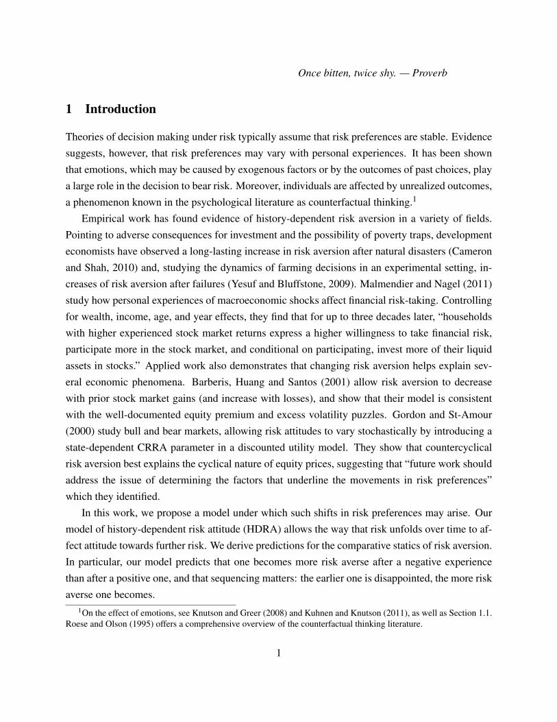
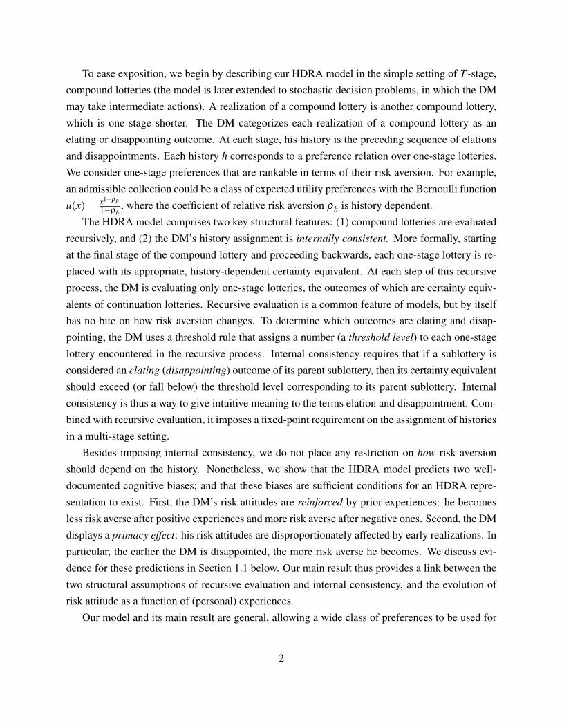


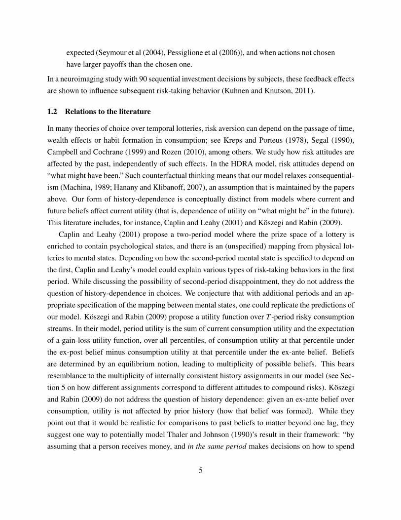
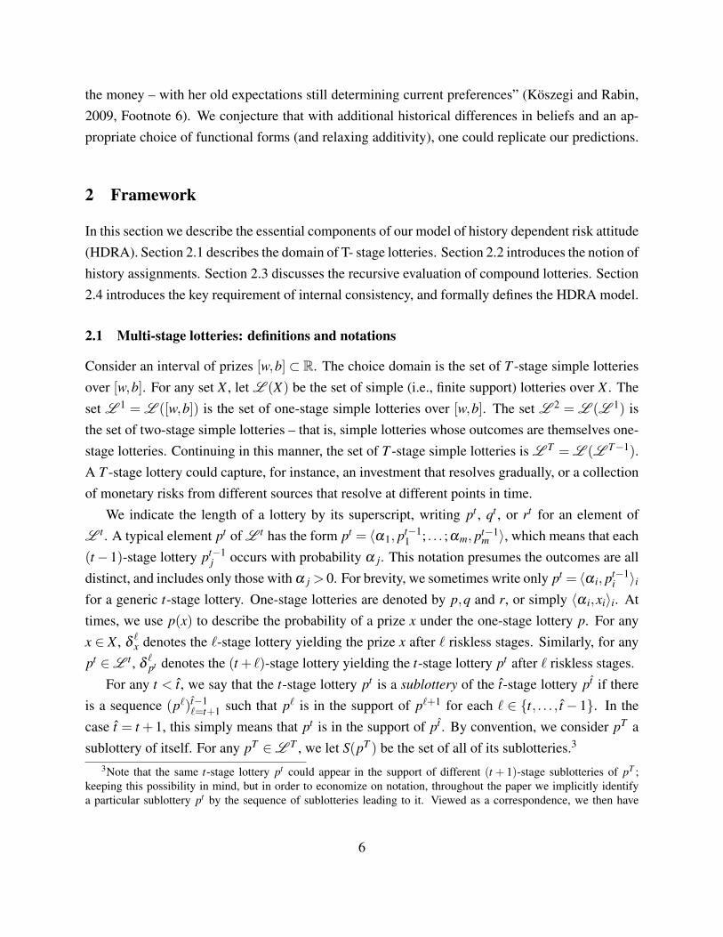


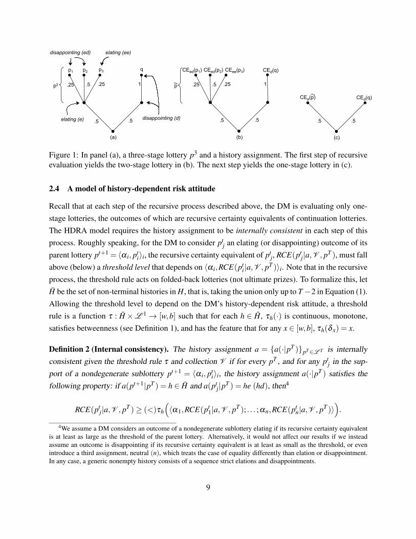
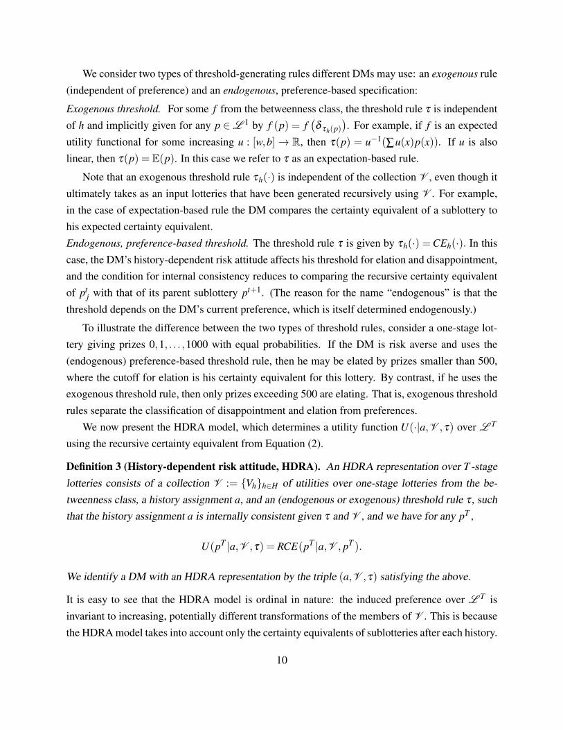


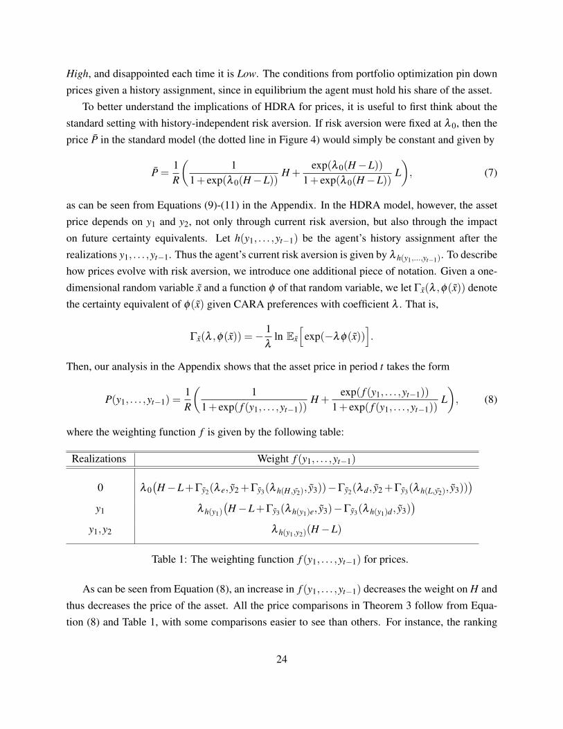


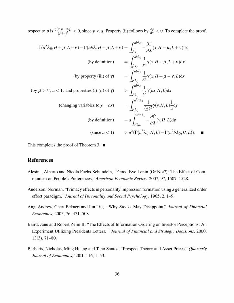


![Bohner Attitude Attitude Change 2011[1]](https://static.documents.pub/doc/80x56/577cdc9c1a28ab9e78aaef04/bohner-attitude-attitude-change-20111.jpg)


