HMMs as Generative Models of Speech [email protected]Workshop on TTS Synthesis 17-JUN-2014 DAIICT Samudravijaya K Tata Institute of Fundamental Research Mumbai [email protected][email protected]Workshop on Text-to-Speech (TTS) Synthesis 16-18 June 2014 Dhirubhai Ambani Institute of Information and Communication Technology Gandhinagar, Gujarat
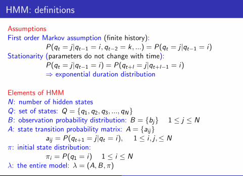
Elements of HMMN: number of hidden statesQ: set of states: Q = {q1, q2, q3, ..., qN}B : observation probability distribution: B = {bj} 1 ≤ j ≤ N
A: state transition probability matrix: A = {aij}aij = P(qt+1 = j |qt = i), 1 ≤ i , j ,≤ N
π: initial state distribution:πi = P(q1 = i) 1 ≤ i ≤ N
λ: the entire model: λ = (A,B , π)
Samudravijaya K Workshop on ASR @BAMU; 14-OCT-11 ASR using Hidden Markov Model : A tutorial 10/26
figures/logos/tifrLogo.eps
3 problems in HMM
1. Matching: Given an observation sequence O = o1, o2, o3, ..., oT , and atrained model λ = (A,B , π), how to efficiently compute the likelihood,P(O|λ) (likelihood of the model λ generating the observationsequence) O?Solution: forward algorithm (use recursion for computational efficiency)Use: Given two models λ1 and λ2, choose λ1 if P(O|λ1) > P(O|λ2)
Samudravijaya K Workshop on ASR @BAMU; 14-OCT-11 ASR using Hidden Markov Model : A tutorial 11/26
figures/logos/tifrLogo.eps
3 problems in HMM
1. Matching: Given an observation sequence O = o1, o2, o3, ..., oT , and atrained model λ = (A,B , π), how to efficiently compute the likelihood,P(O|λ) (likelihood of the model λ generating the observationsequence) O?Solution: forward algorithm (use recursion for computational efficiency)Use: Given two models λ1 and λ2, choose λ1 if P(O|λ1) > P(O|λ2)
2. Optimal path: Given O and λ, how to find the optimal state sequence(Q = q1, q2, q3, ..., qT )?Solution: Viterbi algorithm (similar to DTW)Use: Derive word/phone sequence
3. Training: How to estimate the parameters of the model: λ = (A,B , π)that maximise P(O|λ)?Solution: Forward-backward algorithm.
Samudravijaya K Workshop on ASR @BAMU; 14-OCT-11 ASR using Hidden Markov Model : A tutorial 11/26
An iterative algorithm (Baum-Welch, also known asForward-Backward) is used. The Maximum Likelihood approachguarantees increase of the likelihood of the trained model matchingwith training data with each iteration. To begin with, an initialestimation of parameters of HMMs (A,B , π) is required.
Q: How to get an initial estimation of (λ = {A,B , π}?A: We can estimate parameters if we know the boundaries of everysubword HMM in training utterances.
Samudravijaya K TIFR, [email protected] Introduction to Automatic Speech Recognition 58/76
Training subword HMMs
An iterative algorithm (Baum-Welch, also known asForward-Backward) is used. The Maximum Likelihood approachguarantees increase of the likelihood of the trained model matchingwith training data with each iteration. To begin with, an initialestimation of parameters of HMMs (A,B , π) is required.
Q: How to get an initial estimation of (λ = {A,B , π}?A: We can estimate parameters if we know the boundaries of everysubword HMM in training utterances.
Practical solution: Assume that the durations of all units (phones)are equal. If there are N phones in a training utterance, divide thefeature vector sequence into N equal parts. Assign each part, to aphoneme in the phoneme sequence corresponding to thetranscription of the utterance. Repeat for all training utterances.
Samudravijaya K TIFR, [email protected] Introduction to Automatic Speech Recognition 58/76
Basic units of HMM (phone-like units)
a aA i I u U e e� ao aOa A i I u U e E o Ok K g G Rk kh g gh ng C j J � h j jh njV W X Y ZT Th D Dh Nt T d D nt th d dh np P b B mp ph b bh my r l v f q s hy r l w sh S s hSamudravijaya K TIFR, [email protected] Introduction to Automatic Speech Recognition 54/76
Pronunciation dictionary
* Representing a word as a sequence of units of recognition* Pronunciation rules can be used* Manual verification is necessary
kalam vs kamalkarnaa, pahale, Bhaartiyapause
aage aa g e
aaja aa j
aba a b
abbaasa a bb aa s
aatxha aa t’h
Samudravijaya K TIFR, [email protected] Introduction to Automatic Speech Recognition 55/76
Initial estimation of HMM parameters: an illustration
Let the transcription of the 1st wave file be the following sequenceof words: mera bhaarat mahaan
Let the relevant lines in the dictionary be as follows:bhaarata bh aa r a tmahaana m a h aa nmera m e r aa
The phonemeHMM sequence (of length 16) corresponding to thissentence is sil m e r aa bh aa r a t m a h aa n sil
Samudravijaya K TIFR, [email protected] Introduction to Automatic Speech Recognition 59/76
Initial estimation of HMM parameters: an illustration
Let the transcription of the 1st wave file be the following sequenceof words: mera bhaarat mahaan
Let the relevant lines in the dictionary be as follows:bhaarata bh aa r a tmahaana m a h aa nmera m e r aa
The phonemeHMM sequence (of length 16) corresponding to thissentence is sil m e r aa bh aa r a t m a h aa n sil
If the duration of the wavefile is 1.0sec, there will 98 featurevectors (frame shift = 10msec and frame size = 25msec).
Assign the first 6 feature vectors to “sil” HMM; the next 6 (7through 12) to “m”; the next 6 (13 through 18) to “e”; ... ; thelast 8 feature vectors to “sil”. If HMM has 3 states, assign 2feature vector to each state; compute mean,SD.Assume ai ,j=0.5 if j=i or j=i+1; else assign 0.Samudravijaya K TIFR, [email protected] Introduction to Automatic Speech Recognition 59/76
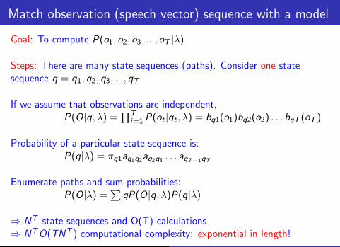
Probability of a particular state sequence is:P(q|λ) = πq1aq1q2aq2q3 . . . aqT−1qT
Enumerate paths and sum probabilities:P(O|λ) =
∑qP(O|q, λ)P(q|λ)
⇒ NT state sequences and O(T) calculations⇒ NT O(TNT ) computational complexity: exponential in length!
Samudravijaya K Workshop on ASR @BAMU; 14-OCT-11 ASR using Hidden Markov Model : A tutorial 12/26
figures/logos/tifrLogo.eps
Forward Algorithm: Intution
1
2
3
i
Stat
es
o3 o_t o_t+1 o_T−1 o_T
Observation sequence
i
j
aij
a2j
a_1j
a3j
aNj
N−1
N
o1 o2
Let αt(i) = P(o1, o2, . . . , ot , qt = i |λ). Then
αt+1(j) =∑N
i=1 αt(i)aijbj(ot+1)
Samudravijaya K Workshop on ASR @BAMU; 14-OCT-11 ASR using Hidden Markov Model : A tutorial 13/26
figures/logos/tifrLogo.eps
Forward Algorithm
Define a forward variable αt(i) as:αt(i) = P(o1, o2, . . . , ot , qt = i |λ)
αt(i) is the probability of observing the partial sequence ( o1, o2, . . . , ot)and ot being generated by i th state (i.e., qt = i).
Induction:Initialization:
α1(i) = πibi (o1)Recursion:
αt+1(j) = [∑N
i=1 αt(i)aij ] bj(ot+1)Termination:
P(O|λ) =∑N
i=1 αT (i)
Samudravijaya K Workshop on ASR @BAMU; 14-OCT-11 ASR using Hidden Markov Model : A tutorial 14/26
figures/logos/tifrLogo.eps
Forward Algorithm
Define a forward variable αt(i) as:αt(i) = P(o1, o2, . . . , ot , qt = i |λ)
αt(i) is the probability of observing the partial sequence ( o1, o2, . . . , ot)and ot being generated by i th state (i.e., qt = i).
Induction:Initialization:
α1(i) = πibi (o1)Recursion:
αt+1(j) = [∑N
i=1 αt(i)aij ] bj(ot+1)Termination:
P(O|λ) =∑N
i=1 αT (i)
Computational complexity: O(N2T )
Use: Match a test speech feature vector sequence with all models. Chooseλi if P(O|λi ) > P(O|λj)∀j
Samudravijaya K Workshop on ASR @BAMU; 14-OCT-11 ASR using Hidden Markov Model : A tutorial 14/26
figures/logos/tifrLogo.eps
Viterbi Algorithm: IntutionProblem 2: Given O and λ, how to find the optimal state sequence(Q = q1, q2, q3, ..., qT ) (Optimal path)?
Samudravijaya K Workshop on ASR @BAMU; 14-OCT-11 ASR using Hidden Markov Model : A tutorial 15/26
figures/logos/tifrLogo.eps
Viterbi Algorithm: IntutionProblem 2: Given O and λ, how to find the optimal state sequence(Q = q1, q2, q3, ..., qT ) (Optimal path)?
Define δt(i) (the highest probability path ending at state i at time t) as:δt(i) = max
q1,q2,...,qt−1
P(q1, q2, · · · , qt = i , o1, o2, . . . , ot |λ)
1
2
3
i
Stat
es
N−1
N
o_t o_t+1
Observation sequence
i
j
aij
a2j
a_1j
a3j
aNj
Viterbi recursion:δt+1(j) = max
iδt(i)aijbj(ot+1)
Contrast the above with the recursion in Forward algorithm:αt+1(j) =
∑N
i=1 αt(i)aijbj(ot+1)
Samudravijaya K Workshop on ASR @BAMU; 14-OCT-11 ASR using Hidden Markov Model : A tutorial 15/26
figures/logos/tifrLogo.eps
Viterbi AlgorithmInitialization:
δ1(i) = πibi(o1), 1 ≤ i ≤ N
ψ1(i) = 0
Recursion:δt(j) = max
1≤i≤N[δt−1(i)aij ] bj(ot)
ψt(j) = argmax1≤i≤N
[δt−1(i)aij ] 2 ≤ t ≤ T , 1 ≤ j ≤ N
Termination:P∗ = max
1≤i≤N[δT (i)]
q∗T = argmax
1≤i≤N
[δT (i)]
Path (optimal state sequence) backtracking:q∗t = ψt+1(q
∗t+1), t = T − 1,T − 2, · · · , 2, 1.
Samudravijaya K Workshop on ASR @BAMU; 14-OCT-11 ASR using Hidden Markov Model : A tutorial 16/26
figures/logos/tifrLogo.eps
Training
Problem 3: Given training data and its transcription, how to estimate theparameters of the model, λ = (A,B , π), that maximises the probability ofrepresentation of training data by the model, P(O|λ)?There is no analytic solution because of its complexity. So, we employExpectation-Maximisation (an iterative) algorithm.
Samudravijaya K Workshop on ASR @BAMU; 14-OCT-11 ASR using Hidden Markov Model : A tutorial 19/26
figures/logos/tifrLogo.eps
Training
Problem 3: Given training data and its transcription, how to estimate theparameters of the model, λ = (A,B , π), that maximises the probability ofrepresentation of training data by the model, P(O|λ)?There is no analytic solution because of its complexity. So, we employExpectation-Maximisation (an iterative) algorithm.
1) Start with an initial (approximate) model, λ0.2) E-step: Using the current model (λ0), compute the expectation of thelikelihood of the training data: P(O|λ) =
∑Ni=1 αT (i).
3) M-step: Re-estimate the parameters (λ = (A,B , π)) so as to maximisethe probability (P(O|λ)).4) Stop if the improvement in log likelihood is insignificant:
P(O|λ)− P(O|λ0) < ∆5) Else, set λ0 ← λ and go to step 2.
The EM algorithm as applied to ASR is known as B-W algorithm; it is alsoknown as Forward-Backward algorithm.
Samudravijaya K Workshop on ASR @BAMU; 14-OCT-11 ASR using Hidden Markov Model : A tutorial 19/26
figures/logos/tifrLogo.eps
Forward-Backward Algorithm: βt(i)
Define a backward variable βt(i) = p(ot+1, . . . , oT |qt = i , λ)
βt(i)Given that we are at node i at time t:
⇒ Sum of probabilities of all paths such thatpartial sequence ot+1, . . . , oT are observed
Samudravijaya K Workshop on ASR @BAMU; 14-OCT-11 ASR using Hidden Markov Model : A tutorial 20/26
Samudravijaya K Workshop on ASR @BAMU; 14-OCT-11 ASR using Hidden Markov Model : A tutorial 21/26
figures/logos/tifrLogo.eps
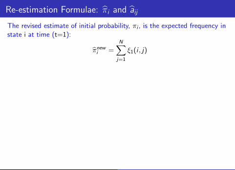
Re-estimation Formulae: πi and aij
The revised estimate of initial probability, πi , is the expected frequency instate i at time (t=1):
πnewi =
N∑
j=1
ξ1(i , j)
Samudravijaya K Workshop on ASR @BAMU; 14-OCT-11 ASR using Hidden Markov Model : A tutorial 22/26
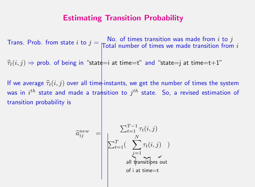
Estimating Transition Probability
Trans. Prob. from state i to j = No. of times transition was made from i to jTotal number of times we made transition from i
τt(i, j) ⇒ prob. of being in “state=i at time=t” and “state=j at time=t+1”
If we average τt(i, j) over all time-instants, we get the number of times the system
was in ith state and made a transition to jth state. So, a revised estimation of
transition probability is
anewij =
∑T−1t=1 τt(i, j)
∑Tt=1(
N∑
j=1
τt(i, j)
︸ ︷︷ ︸all transitions out
of i at time=t
)
WiSSAP 2009: “Tutorial on GMM and HMM”, Samudravijaya K 51 of 88
admin
Pencil
admin
Pencil
admin
Pencil
admin
Pencil
admin
Pencil
admin
Pencil
admin
Pencil
figures/logos/tifrLogo.eps
Re-estimation Formulae: bj(t)
Parameters of State Probability Density FunctionLet us assume that the state output distribution function is Gaussian. Ifthere was just one state j , the maximum likelihood estimation ofparameters would be
µj =1
T
T∑
t=1
ot
Σj =1
T
T∑
t=1
(ot − µj)(ot − µj)′
Samudravijaya K Workshop on ASR @BAMU; 14-OCT-11 ASR using Hidden Markov Model : A tutorial 23/26
figures/logos/tifrLogo.eps
Re-estimation Formulae: bj(t)
Parameters of State Probability Density FunctionLet us assume that the state output distribution function is Gaussian. Ifthere was just one state j , the maximum likelihood estimation ofparameters would be
µj =1
T
T∑
t=1
ot
Σj =1
T
T∑
t=1
(ot − µj)(ot − µj)′
* Difficulty: Speech HMMs have many states.* Speech vector ↔ state mapping is unknown because the state sequenceitself is unknown.* Solution: Assign each speech vector to every state in proportion to thelikelihood of system being in that state when the speech vector wasobserved.
Samudravijaya K Workshop on ASR @BAMU; 14-OCT-11 ASR using Hidden Markov Model : A tutorial 23/26
figures/logos/tifrLogo.eps
Re-estimation Formulae: bj(t)
Let Lj (t) denote the probability of being in state j at time t.
Lj (t) = p(qt = j |O, λ)
=p(qt = j ,O|λ)
p(O|λ)
=αt(i)βt(j)∑
i αT (i)
Samudravijaya K Workshop on ASR @BAMU; 14-OCT-11 ASR using Hidden Markov Model : A tutorial 24/26
figures/logos/tifrLogo.eps
Re-estimation Formulae: bj(t)
Let Lj (t) denote the probability of being in state j at time t.
Lj (t) = p(qt = j |O, λ)
=p(qt = j ,O|λ)
p(O|λ)
=αt(i)βt(j)∑
i αT (i)
Revised estimates of the state pdf parameters are
µj =
∑Tt=1 Lj(t)ot∑Tt=1 Lj(t)
Σj =
∑Tt=1 Lj(t)(ot − µj)(ot − µj)
′
∑Tt=1 Lj(t)
The expected values (estimations) are weighted averages, weights being theprobability of being in state j at time t.
Samudravijaya K Workshop on ASR @BAMU; 14-OCT-11 ASR using Hidden Markov Model : A tutorial 24/26
figures/logos/tifrLogo.eps
Some remarks
Types of HMM* Ergodic Vs left-to-right* Semi-Markov (state duration)* Discriminative models
Implementational Issues* Number of states* Initial parameters* Scaling, addition of logLikelihoods* Multiple observations (tokens/repetitions)* Discrete Vs Continuous probability functions (with GMMs)* Concatenation of smaller HMMs → larger HMM
Samudravijaya K Workshop on ASR @BAMU; 14-OCT-11 ASR using Hidden Markov Model : A tutorial 25/26
figures/logos/tifrLogo.eps
References
◮ Four online tutorials on HMM are listed at< http : //speech.tifr .res.in/tutorials/index .html >
◮ Books: ”Fundamentals of Speech Recognition”, by Lawrence R.Rabiner, B. H. Juang and B.Yegnanarayana, Pearson Education India,2008, Rs. 450; ISBN:9788177585605
◮ Spoken Language Processing : A Guide to Theory, Algorithm andSystem Development, by Xuedong Huang, Alex Acero, Hsiao-WuenHon Year 2001, Prentice Hall PTR; ISBN: 0130226165.
◮ Hidden Markov models for speech recognition; X.D. Huang, Y. Ariki,M.A. Jack. Edinburgh: Edinburgh University Press, c1990.
◮ Statistical methods for speech recognition, F.Jelinek, The MIT Press,Cambridge, MA., 1998.
◮ HMM on MATLAB “HMM toolbox on matlab: Discrete HMMs:training and recognition” by Kevin Murphy, 2005;< http : //www .cs.ubc.ca/ murphyk/Software/HMM/hmm.html >
Samudravijaya K Workshop on ASR @BAMU; 14-OCT-11 ASR using Hidden Markov Model : A tutorial 26/26