46
HMMs and biological sequence analysis

HMMs and biological sequence analysis

HiddenMarkov Model• A Markov chain is a sequence of random variables X1, X2, X3, ... That has the property that the value of the current state depends only on the previous state• Formally P (xi | xi-‐1,…, x1) = P (xi | xi-‐1)• Probability of a sequence P(x) = P(xL,xL-‐1,…, x1) = P (xL | xL-‐1) P (xL-‐1 | xL-‐2)… P (x2 | x1) P(x1) • Usually we consider the set of states to be discrete • Useful for modeling sequences {A,T,C,G}, {L,M,I,V,E,G,…}
X1 X2 Xn-1 Xn

A Markov chain for DNA sequence• Discrete markov chains can be represented as a directed graph
• Define transition probabilities pAA, pAC
• We can generate the some DNA sequence that has a realistic dinucleotide distribution
A C G T
A .300 .205 .285 .210
C .322 .298 .078 .302
G .248 .246 .298 .208
T .177 .239 .292 .292

CpG islands
• Notation: • C-‐G – denotes the C-‐G base pair across the two DNA strands• CpG – denotes the dinucleotide CG
• Methylation process in the human genome:• Very high chance of methyl-‐C mutating to T in CpG
• CpG dinucleotides are much rarer than expected by chance
• Sometimes CpG absence is suppressed • around the promoters of many genes => CpG dinucleotides are much more frequent than elsewhere
• Such regions are called CpG islands• A few hundred to a few thousand bases long
• Problems: • Question 1. Given a short sequence, does it come from a CpG island or not?• Question 2.How to find the CpG islands in a long sequence

CpG Markov chain
Model + A C G T
A .180 .274 .426 .120
C .171 .368 .274 .188
G .161 .339 .375 .125
T .079 .355 .384 .182
Model -‐ A C G T
A .300 .205 .285 .210
C .322 .298 .078 .302
G .248 .246 .298 .208
T .177 .239 .292 .292
The “-‐” model:Use transition matrix A-‐ = (a-‐st), Where: a-‐st = (the probability that t follows s in a non CpG island)
The “+” model:Use transition matrix A+ = (a+st), Where: a+st = (the probability that t follows s in a CpG island)
Is this a CpG island or not?
Use odds ratio
∏
∏−
=+−
−
=++
=−
+= 1
01
1
01
model) (model) (RATIO L
iii
L
iii
xxp
xxp
pp
)|(
)|(
||xx

Where do the parameters come from ?• Given labeled sequence• Tuples {A,+}, {T,+}, {C,+}, … and {A,-‐}, {T,-‐}, {C,-‐}, … • Count all pairs (Xi=a, Xi-‐1=b) with label +, and with label -‐, say the numbers are Nba,+ and Nba,-‐ divide by the total number of + transition observations.• Maximum Likelihood Estimator (MLE) – parameters that maximize the likelihood of the observations• Likelihood
• Probability of data given parameters• Typically very small –the more data there is the smaller its probability• One of increasingly many possibilities
• We can compare the probability of data under different parameters

Digression: MLE• Toy Example• 100 coin flips with 56 heads• What is the probability of getting heads• Compute likelihood of the data from different p• Maximum is at p=0.56• Why bother?
• Complex problems with many parameters the MLE maximizing parameters can be hard to guess
• We can still use this frameworks as long as we can compute the likelihood of the data

Hidden Markov Model• In a hidden Markov model, the state is not directly visible, but the output, dependent on the state, is visible. • Each state has a probability distribution over the possible outputs. • The sequence of outputs generated by an HMM gives some information about the sequence of states.• Formally we have
• State space • Output space • State transition probabilities p(Si+1= t|Si = s) = ast• Emission probabilities p(Xi = b| Si = s) = es(b)
• Still have conditional independence
S1 S2 SL-‐1 SL
x1 x2 XL-‐1 xL
TTTT
1 1 11
( , ) ( , , ; ,..., ) ( | ) ( )i
L
L L i i s ii
p p s s x x p s s e xs x −=
= = ⋅∏K1 1 11
( , ) ( , , ; ,..., ) ( | ) ( )i
L
L L i i s ii
p p s s x x p s s e xs x −=
= = ⋅∏K

Question 2: find CpG islands in a long sequence• Build a single model that combines both Markov chains:
• ‘+’ states: A +, C +, G +, T+ Emit symbols: A, C, G, T in CpG islands
• ‘-‐’ states: A-‐, C-‐, G-‐, T • Emit symbols: A, C, G, T in non-‐islands
• Emission probabilities distinct for the ‘+’ and the ‘-‐’ states – Infer most likely set of states, giving rise to observed emissions
• ‘Paint’ the sequence with + and -‐ states • Hidden Markov Model
• The (+/-‐) states are unobserved• Observe only the sequence

HMM inference problems• Forward Algorithm
• What is the probability that the sequence was produced by the HMM?• What is the probability of a certain state at a particular time given the history of evidence?
• What is the probability of any and all hidden states given the entire observed sequence. Forward-‐backward algorithm• What is the most likely sequence of hidden states? Viterbi • Under what parameterization are the observed sequences most probable? Baum-‐Welch (EM)

Most probable sequence

The Viterbi algorithm• Too many possible paths• Use conditional independence• Dynamical programming algorithm that allows us to compute the most probable path. • similar to the DP programs used to align 2 sequences• Basic DP subproblem: Find the maximal probability the a state l emitted nucleotide i in position x

Viterbi algorithm
•Work in log space• Avoid small numbers• Addition instead of multiplication

Viterbi algorithm

Viterbi algorithm

Profile HMMs for protein families• Pfam is a web-‐based resource maintained by the Sanger Center http://www.sanger.ac.uk/Pfam• Pfam uses the basic theory described above to determine protein domains in a query sequence.• Large collection of multiple sequence alignments and hidden Markov models• Covers many common protein domains and families• Over 73% of all known protein sequences have at least one match• 5,193 different protein families
• Suppose that a new protein is obtained for which no information is available except the raw sequence.• We can go to Pfam to annotate and predict function

Pfam pipeline• Initial multiple alignment of seeds using a program such as Clustal• Alignment hand scrutinized and adjusted• Varying levels of curation (Pfam A, Pfam B)
• Use the alignment to build a profile HMM• Additional sequences are added to the family by comparing the HMM against sequence databases

Pfam Family Types• family – default classification, stating members are related• domain – structural unit found in multiple protein contexts• repeat –domain that in itself is not stable, but when combined with multiple tandem repeats forms a domain or structure• motif – shorter sequence units found outside of domains

Pfam output
HMMs for Protein families
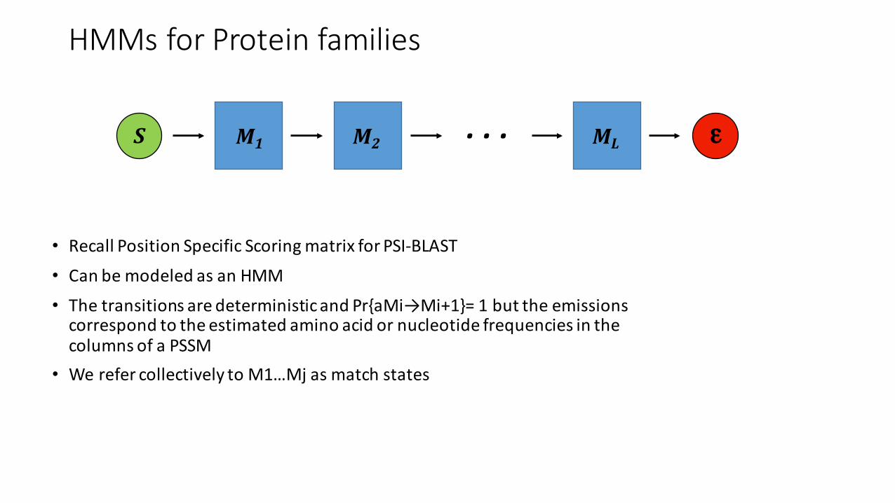
• Recall Position Specific Scoring matrix for PSI-‐BLAST• Can be modeled as an HMM• The transitions are deterministic and Pr{aMi→Mi+1}= 1 but the emissions correspond to the estimated amino acid or nucleotide frequencies in the columns of a PSSM
• We refer collectively to M1…Mj as match states
. . . M1 M2 MLS ε

HMMs for Protein families
• Insertion states correspond to states that do not match anything in the model.• They usually have emission probabilities drawn from the background distribution
• In this case using log-‐odds scoring emissions from the I state do not affect the score
• Only transitions matter• Similar to affine gap penalty
M1 Mj Mj+1S ε. . .
Ij
log aMj→Ij + (k-‐1)·∙log aIj→Ij + log aIj→Mj+1

HMMs for Protein families
• What do we do about deletions?• Can’t allow arbitrary gaps – too many transition probabilities to estimate!
S ε

HMMs for Protein families
• Solution: use silent states to transition between match states
S εMj
Dj

Profile HMM
• Putting it all together– Profile HMM• We have to reliably estimate the parameters from a multiple sequence alignment
S εMj
Dj
Ij
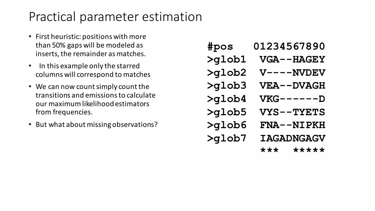
Practical parameter estimation• First heuristic: positions with more than 50% gaps will be modeled as inserts, the remainder as matches.
• In this example only the starred columns will correspond to matches
• We can now count simply count the transitions and emissions to calculate our maximum likelihood estimators from frequencies.
• But what about missing observations?
#pos 01234567890 >glob1 VGA--HAGEY>glob2 V----NVDEV>glob3 VEA--DVAGH>glob4 VKG------D>glob5 VYS--TYETS>glob6 FNA--NIPKH>glob7 IAGADNGAGV
*** *****
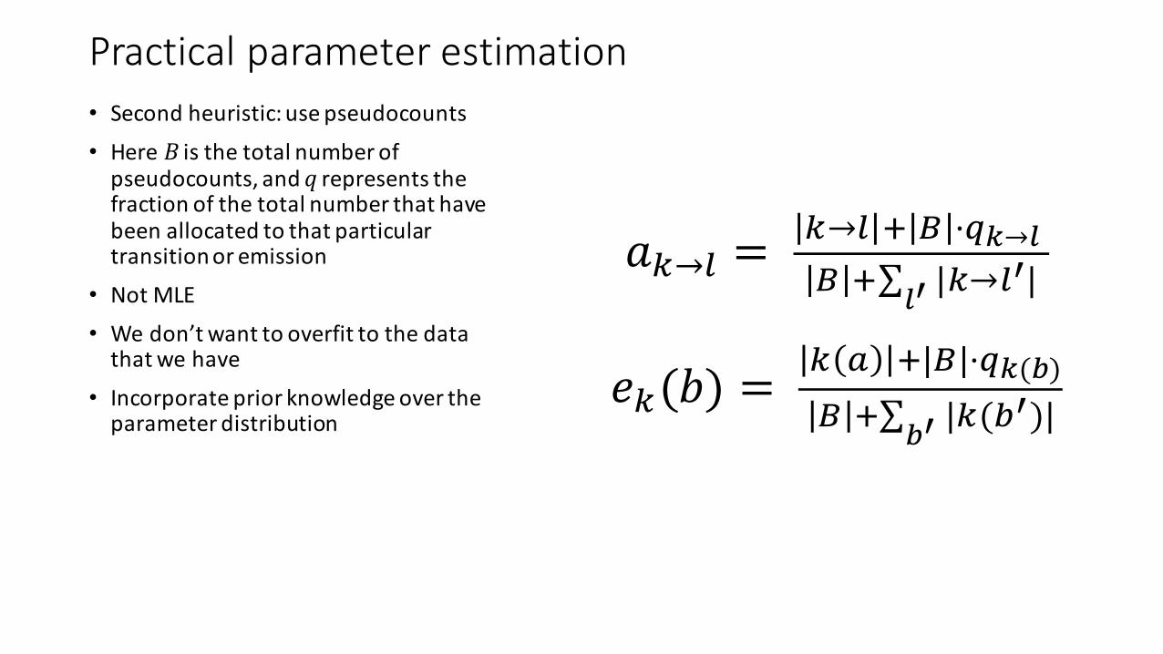
Practical parameter estimation• Second heuristic: use pseudocounts• Here B is the total number of pseudocounts, and q represents the fraction of the total number that have been allocated to that particular transition or emission
• Not MLE• We don’t want to overfit to the data that we have
• Incorporate prior knowledge over the parameter distribution
𝑎"→$ = "→$ ' ( ·*+→, ( '∑ |,/ "→$
/|
𝑒"(𝑏) = " 4 '|(|·*+(5)( '∑ |5/ "(6
/)|

#pos 01234567890 >glob1 VGA--HAGEY>glob2 V----NVDEV>glob3 VEA--DVAGH>glob4 VKG------D>glob5 VYS--TYETS>glob6 FNA--NIPKH>glob7 IAGADNGAGV
*** *****eM1(V) = 6/27, eM1(I) = eM1(F) = 2/27, eM1(all other aa) = 1/27
aM1→M2 = 7/10, aM1→D2 = 2/10, aM1→I1 = 1/10, etc.
Practical parameter estimation

Parameter estimation: unlabeled data• Parameter estimation with a given MSA – labeled data
• Each sequence is labeled with the particular state that it came from
• What if all we have is sequences• Sequences that are not aligned for profile HMM• DNA sequences that are not labeled with CpG (+/-‐)
• We use expectation maximization (EM)• Guess parameters • Expectation: find the structure• Maximization-‐Find the parameters that maximize the data with this structure• Repeat

EM – Canonical Mixture example• Assume we are given heights of 100 individuals (men/women): y1…y100• We know that:• The men’s heights are normally distributed with (μm,σm)• The women’s heights are normally distributed with (μw,σw)
• If we knew the genders – estimation is “easy” • What we don’t know the genders in our data!• X1…,X100 are unknown• P(w),P(m) are unknown

EM• Our goal: estimate the parameters (μm,σm), (μw,σw), p(m)• A classic “estimation with missing data”• (In an HMM: we know the emissions, but not the states!)• Expectation-‐Maximization (EM):• Compute the “expected” gender for every sample height—compare the probabilities of coming from the male and female distributions• Estimate the parameters using ML• Iterate
• HMMS-‐Baum Welch algorithm• Uses forward-‐backward for expectation step

Parameter estimation: EM• Bad news
• Many local minima• Gender height example, usually get the same (correct) answer with all starting points
• Mixture of Gaussians problem:• Want to define X populations in a K dimensional space
under multivariate Gaussian assumption• Chances of getting stuck increase with more complex parameter spaces—complex HMM
• Solution: Use many different starting points• Good news
• Local minima are usually good models of the data• EM does not estimate the number of states. That must be given.
• Often, HMMs are forced to have some transitions with zero probability. This is done by setting aij=0 in initial estimate. Once set to 0 it will not become positive, why?

HMM Topology: state duration
• Consider a simple CpG HMM• How long does our model dwell in a particular state?• Probability of staying in state CpG+ is p• Probability of N residues in CpG+
P(N residues) ~pL-‐‑1
• Exponentially decaying distribution• What is this is not the right distribution
CpG -‐‑S ε
CpG +
p
P
L

HMM Topology: state duration
• 4 states with the same emission probabilities and one internal loop• Guarantees a minimum of 4 consecutive states but still with en exponential tail
etc. etc.

HMM Topology: state duration
• 2 to 6 states• Transition probabilities can be set to model different distributions

Modeling realistic distributions• Two parameters
• Length of chain N• Probability p
• Negative binomial distribution• number of successes in a sequence of independent and identically distributed Bernoulli trials before a specified (non-‐random) number of failures (denoted r) occurs.
1-‐‑p 1-‐‑p 1-‐‑p 1-‐‑p
𝑷 𝒍 = 𝒍 − 𝟏𝒏− 𝟏 𝒑𝒍=𝒏(𝟏 − 𝒑)𝒏

Very flexible distributions

Gene Prediction: Computational Challengeaatgcatgcggctatgctaatgcatgcggctatgctaagctgggatccgatgacaatgcatgcggctatgctaatgcatgcggctatgcaagctgggatccgatgactatgctaagctgggatccgatgacaatgcatgcggctatgctaatgaatggtcttgggatttaccttggaatgctaagctgggatccgatgacaatgcatgcggctatgctaatgaatggtcttgggatttaccttggaatatgctaatgcatgcggctatgctaagctgggatccgatgacaatgcatgcggctatgctaatgcatgcggctatgcaagctgggatccgatgactatgctaagctgcggctatgctaatgcatgcggctatgctaagctgggatccgatgacaatgcatgcggctatgctaatgcatgcggctatgcaagctgggatcctgcggctatgctaatgaatggtcttgggatttaccttggaatgctaagctgggatccgatgacaatgcatgcggctatgctaatgaatggtcttgggatttaccttggaatatgctaatgcatgcggctatgctaagctgggaatgcatgcggctatgctaagctgggatccgatgacaatgcatgcggctatgctaatgcatgcggctatgcaagctgggatccgatgactatgctaagctgcggctatgctaatgcatgcggctatgctaagctcatgcggctatgctaagctgggaatgcatgcggctatgctaagctgggatccgatgacaatgcatgcggctatgctaatgcatgcggctatgcaagctgggatccgatgactatgctaagctgcggctatgctaatgcatgcggctatgctaagctcggctatgctaatgaatggtcttgggatttaccttggaatgctaagctgggatccgatgacaatgcatgcggctatgctaatgaatggtcttgggatttaccttggaatatgctaatgcatgcggctatgctaagctgggaatgcatgcggctatgctaagctgggatccgatgacaatgcatgcggctatgctaatgcatgcggctatgcaagctgggatccgatgactatgctaagctgcggctatgctaatgcatgcggctatgctaagctcatgcgg

Gene Prediction: Computational Challengeaatgcatgcggctatgctaatgcatgcggctatgctaagctgggatccgatgacaatgcatgcggctatgctaatgcatgcggctatgcaagctgggatccgatgactatgctaagctgggatccgatgacaatgcatgcggctatgctaatgaatggtcttgggatttaccttggaatgctaagctgggatccgatgacaatgcatgcggctatgctaatgaatggtcttgggatttaccttggaatatgctaatgcatgcggctatgctaagctgggatccgatgacaatgcatgcggctatgctaatgcatgcggctatgcaagctgggatccgatgactatgctaagctgcggctatgctaatgcatgcggctatgctaagctgggatccgatgacaatgcatgcggctatgctaatgcatgcggctatgcaagctgggatcctgcggctatgctaatgaatggtcttgggatttaccttggaatgctaagctgggatccgatgacaatgcatgcggctatgctaatgaatggtcttgggatttaccttggaatatgctaatgcatgcggctatgctaagctgggaatgcatgcggctatgctaagctgggatccgatgacaatgcatgcggctatgctaatgcatgcggctatgcaagctgggatccgatgactatgctaagctgcggctatgctaatgcatgcggctatgctaagctcatgcggctatgctaagctgggaatgcatgcggctatgctaagctgggatccgatgacaatgcatgcggctatgctaatgcatgcggctatgcaagctgggatccgatgactatgctaagctgcggctatgctaatgcatgcggctatgctaagctcggctatgctaatgaatggtcttgggatttaccttggaatgctaagctgggatccgatgacaatgcatgcggctatgctaatgaatggtcttgggatttaccttggaatatgctaatgcatgcggctatgctaagctgggaatgcatgcggctatgctaagctgggatccgatgacaatgcatgcggctatgctaatgcatgcggctatgcaagctgggatccgatgactatgctaagctgcggctatgctaatgcatgcggctatgctaagctcatgcgg

Eukaryotic Genes

HMM Gene Finder: Veil• A straight HMM Gene Finder• Takes advantage of grammatical structure and modular design
• Uses many states that can only emit one symbol to get around state independence Exon HMM Model
Upstream
Start Codon
Exon
Stop Codon
Downstream
3’ Splice Site
Intron
5’ Poly-‐A Site
5’ Splice Site

GeneScan• a popular and successful gene finder for human DNA sequences is GENSCAN (Burge et al. 1997.)
• Generalized HMM (GHMM)• state may output a string of symbols (according to some probability distribution)• Enter a state
• Output d characters from that state according to some probability
• Transition to the next step
• Explicit intron/exon length modeling
• Increased complexity
• The gene-‐finding application requires a generalization of the Viterbi algorithm.
qi
aiiqj
ajj
qi qj… …pi(d) pj(d)

GeneScan states• N -‐ intergenic region• P -‐ promoter• F -‐ 5’ untranslated region
• Esngl – single exon (intronless) (translation start -‐> stop codon)
• Einit – initial exon (translation start -‐> donor splice site)
• Ek – phase k internal exon (acceptor splice site -‐> donor splice site)
• Eterm – terminal exon (acceptor splice site -‐> stop codon)
• Ik – phase k intron: 0 – between codons; 1 – after the first base of a codon; 2 – after the second base of a codon

Gene finding HMMs• GeneScan can have ~80% accuracy in a compact genome like yeast
• Predicts too many genes for human• GeneScan is data intrinsic –uses only sequence• Many gene prediction programs use additional extrinsic information• Conservation• mRNA evidence
• TwinScan incorporates alignment/conservation information

EGASP:Gene finding programs

EGASP:Gene finding results

EGSP:Performance
• ENCODE based standard
• Relies on human curation
• Evidence based methods may miss some genes


