USWRP Hydrometeorological Testbed’s MultiRadar/MultiSensor (MRMS) Hydro Experiment In coordination with HMT/Flash Flood and Intense Rainfall (FFaIR) Experiment OPERATIONS PLAN July 6 – July 24, 2015 National Weather Center, Hazardous Weather Testbed facilities Norman, OK Updated 30 June 2015
In coordination with HMT/Flash Flood and Intense Rainfall (FFaIR) Experiment
-‐ OPERATIONS PLAN -‐
July 6 – July 24, 2015 National Weather Center, Hazardous Weather Testbed facilities
Norman, OK
Updated 30 June 2015
1. INTRODUCTION The National Oceanic and Atmospheric Administration (NOAA) Hydrometeorological Testbed Program (HMT) is administered by the Office of Water and Air Quality (OWAQ). The HMT promotes hydrometeorological research that will have a short and direct impact on operations within the National Weather Service (NWS), especially in regards to flash flood forecasting. The HMT provides a conceptual framework to foster collaboration between research and operations to test and evaluate emerging technologies and science for NWS operations. The project described herein is unique in that it addresses objectives of the HMT program while leveraging the physical facilities of the Hazardous Weather Testbed (HWT) in Norman, OK. The Multi-‐Radar/Multi-‐Sensor (MRMS) Hydro Experiment (“HMT-‐Hydro” hereafter) will continue into a second year to focus on experimental watches and warnings for hydrologic extremes including flash floods during the warm season. The experiment will be conducted in real time in close coordination with the 3rd annual Flash Flood and Intense Rainfall experiment (FFaIR) at the Weather Prediction Center (WPC). We are seeking feedback from NWS operational forecasters. User comments will be collected during shifts, electronic surveys will be given at the end of the experiment, and discussions will occur during de-‐briefings. Inputs from NWS operational meteorologists and hydrologists are vital to the improvement of the NWS warning process, which ultimately saves public lives and property. The NWS feedback on this test is most important for future development for the NWS and eventual implementation of new applications, display, and product concepts into AWIPS2 and Hazard Services. You are part of a unique team of NOAA scientists, comprised of researchers, technology developers, trainers, and operational forecasters, working together to test new and experimental severe weather warning decision making technology for the NWS. In this operations plan, you will find basic information about the various new technologies and products that we are testing during the 2015 warm season, as well as logistical information about the three -‐week program for all participants. 2. OBJECTIVES The HMT-‐Hydro experiment will be conducted in collaboration with FFaIR to simulate the real-‐time workflow from forecast and guidance products in the 6-‐24 hr timeframe from WPC to experimental flash flood watches and warnings issued in the 0-‐6 hr period. The HMT-‐Hydro team will act as a “virtual, floating forecast office” to shift its area of responsibility on a daily
basis to where heavy precipitation events and concomitant flash flooding is anticipated to occur. The primary scientific goals of the 2015 HMT-‐Hydro experiment are the following:
• Evaluate the relative skill of experimental flash flood monitoring and short-‐term prediction tools from the Flooded Locations And Simulated Hydrographs (FLASH) suite of products: MRMS QPE average recurrence intervals, MRMS QPE-‐to-‐flash flood guidance ratios, and forecast unit streamflow from the hydrologic modeling framework
• Rank the attributes of the FLASH products that will be used to develop regionalized flash flood recommenders
• Determine the benefit of increasing lead time (vs. potential loss in spatial accuracy and magnitude) through the use of extrapolated QPEs and HRRR 0-‐6 hr precipitation forecasts as forcing to FLASH
• Explore the utility of experimental flash flood watches and warnings that communicate both uncertainty (i.e., probability of occurrence) and magnitude (action vs. major flooding events)
• Employ human factors research methods to evaluate the potential use of the Hazard Services software for operational flash flood watch and warning
• Enhance cross-‐testbed collaboration as well as collaboration between the operational forecasting, research, and academic communities on the forecast challenges associated with short-‐term flash flood forecasting
HMT-‐Hydro 2015 will operate in a real-‐time environment in which participants from across the weather enterprise can work together to explore the utility of emerging flash flood monitoring and short-‐term prediction tools for improving flash flood watches and warnings. An overarching theme amongst the testbeds is the rapid testing of the latest observational and modeling capabilities so that they may be improved and optimized for transition to operational decision-‐making within the NWS. Another unique aspect of HMT-‐Hydro is its bridging with FFaIR in order to simulate the collaboration that occurs between the national centers, river forecast centers, and local forecast offices during flash flood events. 3. OPERATIONS The HMT-‐hydro experiment will run Monday-‐Friday for three weeks from July 6 to July 24, 2015. The physical location of the testbed will be in the Hazardous Weather Testbed (HWT) on the 2nd floor of the National Weather Center (NWC). Below is the estimated daily schedule for operations. While we anticipate following the schedule to a certain degree due to coordination
with FFaIR and fixed-‐time reservation of conference rooms, we will also adapt the times due to changes in the weather and to the experiment itself. a. Daily Schedule (all times are in CDT and are subject to change based on the weather) Monday:
11:30am – 1:00pm Working Lunch in the Testbed (get lunch in Flying Cow Café) -‐ Introduction to experimental flash flood products, Anticipated outcomes/Evaluation methodology, WDTD webinar briefing, TBD: Hazard Services, Human factors observational study and consent, “Sandbox” tests with Hazard Services, System Usability Survey,
1:00pm – 1:45pm Weather briefing with FFaIR
2:00pm – 7:15pm Experimental issuance of flash flood watches and warnings
(watches will be valid from 2100 UTC to 0600 UTC, warnings valid from 2100 UTC to 0300 UTC)
??pm Dinner break (time chosen based on weather)
7:15pm – 7:30pm Collection and archiving of materials and notes
Tuesday-‐Thursday: 12:00pm – 1:00pm Lunch at the Flying Cow Café 1:00pm – 1:45pm Weather briefing and post-‐mortem discussion with FFaIR
2:00pm – 3:00pm Evaluation and discussion of prior day’s tools and
watches/warnings ??pm Dinner break (time chosen based on weather) 3:00pm – 7:45pm Experimental issuance of flash flood watches and warnings
(watches will be valid from 2100 UTC to 0700 UTC, warnings valid from 2100 UTC to 0400 UTC)
7:45pm – 8:00pm Collection and archiving of materials and notes, Seminar prep
Friday:
9:00am – 10:00am Evaluation and discussion of prior day’s tools and watches/warnings
10:00am – 11:00pm “Tales from the Testbed” seminar preparation
11:00pm – 12:00pm Working Lunch (“Best practices” questionnaire), Hazard Services
system usability scale survey 12:00pm – 1:00pm “Tales from the Testbed” weekly webinar 1:00pm – 1:15pm Feedback survey 1:15pm – 1:30pm Group photo 1:30pm Adjourn
b. Activity Descriptions Visitor Welcome – Participants who are NWS employees are reminded to bring their NOAA CAC cards in order to pass through security. Foreign Nationals need to contact the project PI, JJ Gourley ([email protected]), well in advance in order to get the required clearance.
The NWC is a University of Oklahoma building that houses several NOAA facilities. The HMT-‐Hydro Operations Area will be held in the HWT and is considered a secure NOAA location. Therefore, certain NOAA security requirements are in effect for visitors to the HMT-‐Hydro experiment. All NOAA employees are required to visibly wear, at all times, their NOAA identification badges. Non-‐NOAA visitors must check in each day with the security desk using their state-‐issued IDs at the 1st floor entrance to obtain a daily visitor pass.
The NOAA participants will be issued one white magnetic key card which will allow entrance into certain secure locations in the NWC. These include the NOAA main hallway (with access to a kitchenette) and the HMT-‐Hydro operations area in the HWT. Each door card has an associated 4-‐number PIN that is keyed into the lock pad in order to gain entry. Participants must return their door key cards and visitor badges to the Operations Coordinator before they leave the NWC on Friday to return home, as these will be recycled each week for the next set of participants.
Weather Briefing – The weather briefing will be primarily directed by FFaIR. HMT-‐Hydro participants will join the briefing (via GotoMeeting and conf call) in the HWT. The primary goals of the briefing are to: 1) conduct a post-‐mortem on experimental products issued the prior day by overlaying all flash flood observations on the guidance, watches, and warnings, 2) provide present synopsis of rainfall and flooding for situational awareness, and 3) summarize the day’s model-‐based forecasts of heavy rainfall and guidance for probabilistic flash flooding.
Introduction – Description of the FLASH experimental products are provided in Appendix 1 at the end of this document. Participants are encouraged to familiarize themselves with the products in advance of the experiment. The experiment coordinators will use the Monday 1:45 time slot to describe the products in more detail and be able to answer participants’ questions. We will solicit participant feedbacks at this point because the materials provided in Appendix 1 (and also on the Vlab Wiki) and the powerpoints will eventually be used to develop official Warning Decision Training Division (WDTD) training materials. We will also cover the anticipated outcomes the researchers expect with the experiment. While we hope to use Hazard Services to display experimental FLASH products as well as operational model and observational products to issue experimental watches/warnings, we are also prepared to use the D2D perspective in AWIPS2 and WarnGen to issue experimental watches and warnings. Evaluations of the prior day’s tools and experimental products will be accomplished using the http://flash.ou.edu website. Thus, we ask the participants to familiarize themselves with the real-‐time display of products and observations through the website. All evaluations during the HMT-‐Hydro experiment will have a subjective component. We will present to the participants our strategies for evaluating the forecast tools, ranking their regional attributes, and evaluating skill and characteristics of the experimental watches and warnings. The latter two will also include information about uncertainty and magnitude. Lastly, a PhD student has received authorization from the University of Oklahoma’s Institutional Review Board to conduct a usability evaluation of the Hazard Services system that will be conducted during the training activities on Monday. In addition to completing the planned Hazard Services training, the evaluation will involve completing a questionnaire about the software’s user interface. Participation is optional, and an opportunity to learn more about the study will be available before deciding whether or not to participate. Experimental Watches/Warnings – We plan on using Hazard Services to issue the experimental products beginning at approximately 2000 UTC, depending on the day’s weather and schedule. The focus region for product issuance will initially correspond to the FFaIR guidance, but is expected to change based on the observations. The experimental watches and warnings are intended to approximate the responsibilities of a local forecast office, but with the ability to
adapt its county warning area. In the event of multiple flash flooding events occurring in separate regions of the US, the experimental domain should prioritize its single domain based on anticipated impacts and perhaps population density (in order to obtain dense reports). It is understood that operational procedures differ from office-‐to-‐office in regard to the issuance of flash flood watches. The HMT-‐Hydro experiment will adopt a nationally consistent approach that will be based on observed precipitable water values, short-‐term QPFs from the HRRR, radar trends, observed river states from available USGS stations (http://waterwatch.usgs.gov/?id=ww_flood) and FLASH products, rather than model guidance of heavy rainfall. Thus, it will more closely mimic the lead-‐times and space-‐time scales typically seen with severe weather watches. The experimental watches/warnings will differ from those issued in operations in that they will include estimates of probability of occurrence corresponding to two flash flooding magnitudes (action, major).
Subjective Evaluation – Because the evaluations performed in HMT-‐Hydro involve subjectivity, we have devoted one hour each day for this important activity. We expect a great deal of information to be inserted into the comments section following each evaluation. First, all available flash flooding observations from NWS local storm reports, citizen-‐scientist reports from the meteorological Phenomena Indication Near the Ground (mPING) project, targeted reports from the public in the Severe Hazards And Verification Experiment (SHAVE), and USGS streamflow observations will be used together to rank the MRMS QPE, QPE average recurrence intervals, QPE-‐to-‐flash flood guidance ratios, and CREST unit streamflow in terms of 1) spatial extent of flooding and 2) magnitude. The ADSTAT-‐forced and HRRR-‐forced CREST unit streamflow products will be evaluated to determine 1) their accuracy in comparison to the MRMS-‐forced forecasts and 2) amount of lead time provided. The experimental watches are warnings will be evaluated in terms of their communication of uncertainty and magnitude. Probabilities assigned to watches/warnings are meant to correspond to an observation occurring within them at the same frequency. All flash flooding observations will be employed to assess whether an event falls into the action or major category. Note that both SHAVE and mPING reports subdivide the flash flooding reports as follows: 1) river/creek overflowing, cropland/yard/basement flooding, 2) street/road flooding or closure, vehicles stranded, 3) homes/buildings with water in them, and 4) homes/buildings/vehicles swept away. Reports of 1 and greater will be used to validate an action flood, while a 3 or 4 is required for a major flood. The major flood category also includes personal impacts such as rescues, evacuations, injuries, and fatalities. If a flood is captured by a USGS stream gauge, then the reported flood stage can be used to validate the magnitude associated with the watch/warning. Experimental watches/warnings will be compared and contrasted to operationally issued products.
“Tales from the Testbed” Webinar – Participants will be given time throughout the forecast process Monday-‐Thursday to archive products and notes. The logistics facilitator will work with the forecasters each day during the week of operations to help them capture images and develop their contribution to the end-‐of-‐week webinars. It is encouraged that many images are captured, and used as Blog entries, as this will make the collation of the images for the webinar that much easier. The final 15 minutes of the Monday through Wednesday and 30 minutes of the Thursday shifts will be devoted to gathering all the images for the week and coming up with a strategy for an initial draft of the presentation. Forecasters will be given an hour on Friday morning from 10-‐11am to finalize their presentation and practice. After lunch, from 12-‐1 pm CDT, we will regroup and present the forecasters’ experience throughout the experiment in a webinar setting. The WDTD will facilitate the webinars. The forecasters will have approximately 22 minutes to discuss their key takeaways that week. The topic can be a specific case study, functionality of Hazard Services, the experimental tools, or the experimental products that were issued. 15 minutes will remain for audience feedback and questions. The audience is anyone with an interest in what we are doing to improve flash flood monitoring and prediction observations/tools and NWS flash flood watch and warning products. Anticipated audience included NWS field personnel, regional and national headquarters personnel, and our other stakeholders in NOAA and elsewhere.
Feedback Survey – At the end of the week, project participants will fill out an online feedback survey. Last year, we found these feedbacks to be particularly useful to us. Once again, participant feedbacks will be used immediately to improve the experimental design for coming days, weeks and next year. 4. PRODUCTS The subjective evaluations will focus on NSSL’s MRMS and FLASH products that are being developed and improved for rapid transition to operational use in the NWS. The primary flash flood monitoring and prediction tools to be evaluated include MRMS QPEs, QPE average recurrence intervals, QPE-‐to-‐FFG ratios, and CREST unit streamflow forecast products. Table 1 summarizes the experimental and operational flash flood observations and tools that will be the focus of the HMT-‐Hydro experiment.
Table 1. Summary of flash flood observations and tools to be evaluated during HMT-‐Hydro for a three-‐week experimental period in July 2015. Provider Product Description Flash Flood Observations NWS Local Storm Reports Operational reports of flash flooding used to
validate warnings NSSL mPING Citizen-‐scientist reports of flash flooding at 4
levels of severity NSSL SHAVE Targeted reports from the public on details of
flash flooding at high resolution USGS/NWS/NSSL Streamflow Measurements of streamflow that have
exceeded flood stage or a nominal return period flow (e.g., 5-‐yr return) in small, gauged basins
Flash Flood Monitoring and Prediction Tools (primarily for issuance of warnings) NSSL MRMS QPE Quantitative precipitation estimates from
radar-‐only algorithms at multiple accumulation periods (2 min to 6 hr)
NSSL QPE recurrence interval Compares MRMS QPE to 30-‐min, 1-‐, 3-‐, 6-‐, 12, and 24-‐hr precipitation frequencies from NOAA Atlas 14*. The product indicates when a particular return period threshold is exceeded by estimated rainfall. (available every 5 minutes)
RFCs/WPC/NSSL QPE-‐to-‐FFG ratio Compares a 1-‐, 3-‐, and 6-‐hr rolling sum of MRMS QPE to the most recent issuance of 1-‐, 3-‐, and 6-‐hr FFG** (available every 5 minutes)
NSSL Max unit streamflow Maximum unit streamflow forecast by CREST during an interval spanning 30 min prior to valid time to 6 hrs after valid time (available at 0, 15, 30, and 45 minutes after every hour)
Short-‐term Forecasting Tools (primarily for issuance of watches) NSSL/GSD Precipitable Water
Analysis RAP analysis of precipitable water (available hourly)
NSSL/GSD Precipitable Water Anomaly Analysis
Comparison of above produce to sounding-‐observed values from 1948 to 2010. Values are provided as a percentile.
National Water Center
ADSTAT forecasts Extrapolated QPEs provided to FLASH on 3 km/hourly basis for a lead time of 0-‐6 hrs.
GSD HRRR forecasts QPFs provided to FLASH on 3 km/hourly basis for a lead time of 0-‐6 hrs
*NOAA Atlas 14 does not yet include precipitation frequency estimates for the Northwestern US, New England, New York, or Texas.
**RFCs typically update FFG at synoptic (00 UTC and 12 UTC) and sub-‐synoptic (06 UTC and 18 UTC) times, but the FLASH server queries all RFCs once an hour for FFG updates. During heavy rainfall events some RFCs produce intermediate FFG products and hourly queries ensure that FLASH catches these intermediate FFG issuances. The FFG product displayed in FLASH is a national mosaic. There are different methodologies used to produce FFG across the country (including gridded and lumped FFG as well as flash flood potential index) and so discontinuities in FFG values across RFC boundaries may exist.
5. PERSONNEL a. Officers Jonathan J. Gourley Principal Investigator [email protected] Gabriel Garfield NSSL HWT Liaison [email protected] Steven Martinaitis Operations Coordinator [email protected] Zachary L. Flamig Information Technology Coordinator [email protected] Michael Bowlan WDTD “Tales from the Testbed” Facilitator [email protected] b. Weekly Coordinators There will be one primary weekly coordinator for each of the three weeks of testbed operations. The weekly coordinator will be responsible for facilitating the operational activities of the week, including:
• Welcoming the participants and giving a tour of the building • Facilitating the daily weather briefing with FFaIR • Coordinating daily forecast operations • Directing the daily subjective evaluations and filling out the questionnaire • Helping forecasters in preparation of materials for the “Tales from the Testbed”
Webinars • Disseminating the exit survey
During operational periods of the experiment, the weekly coordinator will work with the Operations Coordinator on the following:
• Ensuring that the principle scientists are interacting with the forecasters • Identifying separate forecast domains and teams • Ensuring the smooth running of the technology and alerting various IT personnel when
there are problems • Coordinating dinner time • Ensuring “crowd and noise control” • Making sure the ops area is clean and all computers logged off at end of shift
The following are the weekly coordinators: HMT-‐Hydro Week 1 (6-‐10 July) Elizabeth Argyle [email protected] HMT-‐Hydro Week 2 (13-‐17 July) Ami Arthur [email protected] HMT-‐Hydro Week 3 (20-‐24 July) Race Clark [email protected] Cell phone numbers for experiment officers and weekly coordinators will be provided to participants in hard copy form upon their arrival at the National Weather Center. c. Forecaster Participants The forecasters, representing a geographically diverse set of Weather Forecast Offices (WFOs) and River Forecast Centers (RFCs) will be available full-‐time for the entire weekly shift schedule. There will be at least two forecast teams that will focus on different domains, depending on the daily weather scenario. Forecasters will be issuing watches and warnings using Hazard Services (or WarnGen on AWIPS2 as a backup) and evaluating the tools and forecast products. HMT-‐Hydro Week 1 (6-‐10 July)
• Adrienne Leptich -‐ WFO Upton, NY • Jeremy Wesely -‐ WFO Hastings, NE • Pamela Szatanek -‐ WFO Elko, NV • Jason Elliott -‐ WFO Sterling, VA • Peter Corrigan -‐ WFO Blacksburg, VA
• Wayne Ruff -‐ WFO Norman, OK HMT-‐Hydro Week 2 (13-‐17 July)
• Barrett Smith -‐ WFO Raleigh, NC • Alicia Miller -‐ WFO Pittsburgh, PA • Scott Lincoln -‐ Lower Mississippi RFC • Leonard Vaughan -‐ WFO Columbia, SC • Marcus Austin -‐ WFO Norman, OK • Megan Terry -‐ WFO Springfield, MO
HMT-‐Hydro Week 3 (20-‐24 July)
• Jared Allen -‐ WFO San Antonio, TX • Shawn DeVinny -‐ WFO Chanhassen, MN • Brett Albright -‐ WFO San Diego, CA • Christina Barron -‐ WFO Corpus Christi, TX • Christopher Rasmussen -‐ WFO Tuscon, AZ • Krizia Negron -‐ WFO Key West, FL
d. Observers/Additional Participants We anticipate participation or observations from “participants of opportunity” who may be in town for other meetings. We have enough space to accommodate additional participants and welcome those from NOAA headquarters, academia, private sector, and beyond to take part in the experiment. However, please contact the Principal Investigator and Operations Coordinator prior to arriving.
APPENDIX 1: Product Descriptions of Experimental MRMS-‐FLASH Products
CREST Maximum Unit Streamflow (CREST Max Unit
Streamflow)
Short Description: Forecast of maximum unit streamflow from -30 min to +6 hrs, based on modeled stream flows from the Coupled Routing and Excess STorage (CREST) distributed hydrologic model
Alternate Names: CREST Max Unit Q, Max Unit Q, FLASH Max Unit Q
Input Sources: MRMS quality-controlled radar-only Precipitation Rate, RAP temperature analysis
Availability: Q2FY16 (v11)
Users: NWS WFOs, NWS RFCs, NWS NCEP WPC
Long Description: The forward simulation comes from feeding near real-time precipitation data to the distributed hydrologic model (DHM) and allowing the model to run forward for 6 hours. Currently, the model assumes that all rainfall stops at the model initialization time. Topographical, land cover, land use, and soil type information is used by the model to infiltrate and route precipitation downstream once it
reaches the land surface. Additionally, temperature analyses from the RAP model are used to calculate potential evapotranspiration for forcing to the model. Thus the output from the DHM is a flow rate/discharge at every grid cell. These time-integrated maximum discharge values are then normalized at each grid cell by the associated drainage area, producing a unit discharge value. The CREST model serves as the DHM for this product (Wang et al. 2011). While the water balance parameters are not calibrated using observed streamflow, they are based on spatially distributed maps of land use, soil characteristics, and digital elevation model derivatives. The model is primarily designed to predict flood stages, and not the details of the hydrograph such as baseflow, recession limb, etc.
Applications: CREST Max Unit Streamflow is used to diagnose areas of flash flooding potential over a 6.5-hr forecast window. CREST Max Unit Streamflow can also identify the relative severity of potential flash flooding impacts. Areas of contiguous pixels with high values (~ 10 m3/s/km2) are usually a cause for concern; a single pixel or a handful of isolated pixels with large values may not be indicative of a flash flooding threat.
Example Images:
This is output from the FLASH web interface showing the forecast maximum unit streamflow over Houston, TX from 13:30 UTC to 10:00 UTC on 26 May 2015. Note the numerous pixels with values approaching and often exceeding 10 m3/s/km2. This was a catastrophic flash flood that resulted in approximately 20 fatalities throughout the city. As time marches on, the main threat moves from the overland pixels into the channel network and propagates downstream.
Issues: This product relies heavily on precipitation estimates from weather radar. Areas with complex topography, beam blockage, wind farms, and other difficulties that contaminate QPE will be adversely affected. Further, the model does not presently simulate snowmelt and assumes that all rivers remain
free from diversions, dams, withdrawals, dikes, and any other anthropogenic influence.
References:
Wang, J., Y. Hong, L. Li, J. J. Gourley, S. Khan, K. Yilmaz, R. Adler, F. Policelli, S. Habib, D. Irwn, A. Limaye, T. Korme, and L. Okello, 2011: The coupled routing and excess storage (CREST) distributed hydrological model. Hydrolog. Sci. J., 56, 84-98.
CREST Maximum Streamflow (CREST Max Streamflow) Short Description: Forecast of maximum streamflow from -30 min to +6 hrs, based on modeled stream flows from the Coupled Routing and Excess STorage (CREST) distributed hydrologic model
Alternate Names: CREST Max Streamflow, FLASH Streamflow
Input Sources: MRMS quality-controlled radar-only Precipitation Rate, RAP temperature analysis
Availability: Q2FY16 (v11)
Users: NWS WFOs, NWS RFCs, NWS NCEP WPC
Long Description: Distributed hydrologic models (DHMs) are used to simulate river or stream flow based on rainfall, evapotranspiration, topography, soil characteristics, and other land properties. CREST (Coupled Routing and Excess STorage) is the DHM used to make this product (Wang et al. 2011). A digital elevation model (DEM) and flow accumulation map (FAC) are used by the model to route water from precipitation downstream once it has reached and infiltrated into the land surface. Soil and land use information are used in the model to determine how much of the surface water
will become overland flow, and a kinematic wave solution to the Saint-Venant Equations is used to route the channelized water downstream. Temperature analyses from the RAP model are used to calculate potential evapotranspiration for forcing to the model. Currently, the model uses observed rainfall from the MRMS Radar-only product at the model initialization time. Some experiments will use QPF forcing at future time steps instead of assuming there is zero rainfall in the future. The output from the DHM is a flow rate/discharge at every grid cell.
Applications: CREST Maximum Streamflow can be used to visualize stream and river networks and to identify broad areas where relatively high flows are occurring. This product can be directly compared to streamflow measured at USGS gauging sites.
Example Images:
This is output from the FLASH web interface showing the forecast maximum streamflow over Houston, TX from 13:30 UTC to 10:00 UTC on 26 May 2015. A contiguous area of pixels with streamflow values exceeding 10 m3/s are noted over the city. This indicates the overland pixels are all producing overland flow due to the impervious surfaces over the city. This product shows much greater values in the nearby perennial rivers. Without context or knowledge of the amount of water required to cause flooding overland or in the channels in this area, this output cannot easily be used to forecast a flash flooding event by itself.
Issues: This product relies heavily on precipitation estimates from weather radar. Areas with complex
topography, beam blockage, wind farms, and other difficulties that contaminate QPE will be adversely affected. Further, the model does not presently simulate snowmelt and assumes that all rivers remain free from diversions, dams, withdrawals, dikes, and any other anthropogenic influence.
The water balance parameters of the CREST model are based on a-priori physiographic maps and are not optimized using streamflow observations. The kinematic wave parameters have been derived at USGS gauge stations and are modeled for all channel pixels. In any case, as with any uncalibrated model, streamflow values at a particular grid cell may differ from the observed river conditions. The CREST model has primarily been designed to forecast peakflows, so large model-observation discrepancies can occur, especially when examining details such as baseflow or recession limb of the hydrograph. This product should not be used in isolation to forecast floods or flash floods. Instead, it should be used to investigate and confirm model-based errors that will propagate to the CREST Max Unit Streamflow and Threshold Exceedance products.
References:
Wang, J., Y. Hong, L. Li, J. J. Gourley, S. Khan, K. Yilmaz, R. Adler, F. Policelli, S. Habib, D. Irwn, A. Limaye, T. Korme, and L. Okello, 2011: The coupled routing and excess storage (CREST) distributed hydrological model. Hydrolog. Sci. J., 56, 84-98.
CREST Soil Moisture Short Description: Analysis of the soil saturation (%) from the Coupled Routing and Excess STorage (CREST) hydrologic model
Input Sources: MRMS quality-controlled radar-only Precipitation Rate, RAP temperature analysis
Availability: Q2FY16 (v11)
Users: NWS WFOs, NWS RFCs, NWS NCEP WPC
Long Description: One of the key tasks in hydrologic modeling is quantifying the amount of moisture present in the soil within the model domain. This product expresses top-layer soil moisture as a percentage of saturation. Low soil moisture values imply that more water storage space is available in the soil layer; therefore a greater fraction of precipitation will infiltrate into the soil and be unavailable to cause surface runoff. High soil moisture values typically result in greater surface runoff and thus greater flash flood potential. In this product, the output is from the CREST model (Wang et al. 2011).
Applications: CREST Soil Moisture can be used to distinguish between broad areas of wetter or drier soil
conditions. This product can help identify areas that have recently received rainfall and are at an increased risk of flash flooding due to moist soil conditions.
Example Images:
This is an analysis of soil saturation over the south-central US from the CREST hydrologic model valid at 06 UTC on 24 May 2015. Values are expressed as a percentage of saturation. Areas presently or recently impacted by heavy rainfall have values > 50% of saturation.
Issues: This product is a raw model field and has not been post-processed so it may bear little resemblance to in situ or remotely sensed soil moisture observations. This field should primarily be used to for diagnosing issues with or further investigating outputs from the CREST maximum streamflow and maximum unit streamflow products.
References:
Wang, J., Y. Hong, L. Li, J. J. Gourley, S. Khan, K. Yilmaz, R. Adler, F. Policelli, S. Habib, D. Irwn, A. Limaye, T. Korme, and L. Okello, 2011: The coupled routing and excess storage (CREST) distributed hydrological model. Hydrolog. Sci. J., 56, 84-98.
SAC Maximum Unit Streamflow (SAC Max Unit Streamflow)
Short Description: Forecast of maximum unit streamflow from -30 min to +6 hrs, based on modeled stream flows from the SACramento family(SAC)of hydrologic models
Input Sources: MRMS quality-controlled radar-only Precipitation Rate, RAP temperature analysis
Availability: Q4FY16 (v12)
Users: NWS WFOs, NWS RFCs, NWS NCEP WPC
Long Description: The forward simulation comes from feeding near real-time precipitation data to the distributed hydrologic model (DHM) and allowing the model to run forward for 6 hours. Currently, the model uses observed rainfall from the MRMS Radar-only product at the model initialization time. Some experiments will use QPF forcing at future time steps instead of assuming there is zero rainfall in the future. Topographical, land cover, land use, and soil type information is used by the model to infiltrate and route precipitation downstream once it reaches the land
surface. Additionally, temperature analyses from the RAP model are used to calculate potential evapotranspiration for forcing to the model. Thus the output from the DHM is a flow rate/discharge at every grid cell. These time-integrated maximum discharge values are then normalized at each grid cell by the associated drainage area, producing a unit discharge value. The SAC model serves as the DHM for this product(Burnash et al. 1973). While the water balance parameters are not calibrated using observed streamflow, they are based on spatially distributed maps of land use, soil characteristics, and digital elevation model derivatives. The model is primarily designed to predict flood stages, and not the details of the hydrograph such as baseflow, recession limb, etc.
Applications: SAC Max Unit Streamflow is used to diagnose areas of flash flooding potential over a 6.5-hr forecast window. SAC Max Unit Streamflow can also identify the relative severity of potential flash flooding impacts. Areas of contiguous pixels with high values (~ 10 m3/s/km2) are usually a cause for concern; a single pixel or a handful of isolated pixels with large values may not be indicative of a flash flooding threat.
Example Images:
This is output from the FLASH web interface showing the forecast maximum unit streamflow over Houston, TX from 3:30 UTC to 10:00 UTC on 26 May 2015. Note the numerous pixels with values approaching and often exceeding 4-5 m3/s/km2. This was a catastrophic flash flood that resulted in approximately 20 fatalities throughout the city. As time marches on, the main threat moves from the overland pixels into the channel network and propagates downstream.
Issues: This product relies heavily on precipitation estimates from weather radar. Areas with complex topography, beam blockage, wind farms, and other difficulties that contaminate QPE will be adversely affected. Further, the model does not presently
simulate snowmelt and assumes that all rivers remain free from diversions, dams, withdrawals, dikes, and any other anthropogenic influence.
References:
Burnash, R. J. C., R. Ferral, R. McGuide, 1973: A generalized streamflow simulation system – conceptual modeling for digital computers. US Department of Commerce, National Weather Service and State of California, Department of Water Resources.
SAC Maximum Streamflow (SAC Max Streamflow) Short Description: Forecast of maximum streamflow from -30 min to +6 hrs, based on modeled stream flows from the SACramento family(SAC)of hydrologic models
Input Sources: MRMS quality-controlled radar-only Precipitation Rate, RAP temperature analysis
Availability: Q4FY16 (v12)
Users: NWS WFOs, NWS RFCs, NWS NCEP WPC
Long Description: Distributed hydrologic models (DHMs) are used to simulate river or stream flow based on rainfall, evapotranspiration, topography, soil characteristics, and other land properties. The SAC model serves as the DHM for this product(Burnash et al. 1973). A digital elevation model (DEM) and flow accumulation map (FAC) are used by the model to route water from precipitation downstream once it has reached and infiltrated into the land surface. Soil and land use information are used in the model to determine how much of the surface water will become overland flow, and a kinematic wave solution to the Saint-Venant
Equations is used to route the channelized water downstream. Temperature analyses from the RAP model are used to calculate potential evapotranspiration for forcing to the model. Currently, the model assumes that all rainfall stops at the model initialization time. The output from the DHM is a flow rate/discharge at every grid cell.
Applications: SAC Maximum Streamflow can be used to visualize stream and river networks and to identify broad areas where relatively high flows are occurring. This product can be directly compared to streamflow measured at USGS gauging sites.
Example Images:
This is output from the FLASH web interface showing the forecast maximum streamflow over Houston, TX from 3:30 UTC to 10:00 UTC on 26 May 2015. A contiguous area of pixels with streamflow values exceeding 5 m3/s are noted over the city. This indicates the overland pixels are all producing overland flow due to the impervious surfaces over the city. This product shows much greater values in the nearby perennial rivers. Without context or knowledge of the amount of water required to cause flooding overland or in the channels in this area, this output cannot easily be used to forecast a flash flooding event by itself.
Issues: This product relies heavily on precipitation estimates from weather radar. Areas with complex topography, beam blockage, wind farms, and other difficulties that contaminate QPE will be adversely affected. Further, the model does not presently simulate snowmelt and assumes that all rivers remain free from diversions, dams, withdrawals, dikes, and any other anthropogenic influence.
The water balance parameters of the SAC model are based on a-priori physiographic maps and are not optimized using streamflow observations. The kinematic wave parameters have been derived at USGS gauge stations and are modeled for all channel pixels. In any case, as with any uncalibrated model, streamflow values at a particular grid cell may differ from the observed river conditions. The SAC model has primarily been designed to forecast peakflows, so large model-observation discrepancies can occur, especially when examining details such as baseflow or recession limb of the hydrograph. This product should not be used in isolation to forecast floods or flash floods. Instead, it should be used to investigate and confirm model-
based errors that will propagate to the CREST Max Unit Streamflow and Threshold Exceedance products.
References:
Burnash, R. J. C., R. Ferral, R. McGuide, 1973: A generalized streamflow simulation system – conceptual modeling for digital computers. US Department of Commerce, National Weather Service and State of California, Department of Water Resources.
SAC Soil Moisture Short Description: Analysis of the soil saturation (%) from the SACramento family(SAC)of hydrologic models
Input Sources: MRMS quality-controlled radar-only Precipitation Rate, RAP temperature analysis
Availability: Q4FY16 (v12)
Users: NWS WFOs, NWS RFCs, NWS NCEP WPC
Long Description: One of the key tasks in hydrologic modeling is quantifying the amount of moisture present in the soil within the model domain. This product expresses top-layer soil moisture as a percentage of saturation. Low soil moisture values imply that more water storage space is available in the soil layer; therefore a greater fraction of precipitation will infiltrate into the soil and be unavailable to cause surface runoff. High soil moisture values typically result in greater surface runoff and thus greater flash flood potential. In this product, the output is from the SAC model (Burnash et al. 1975).
Applications: SAC Soil Moisture can be used to distinguish between broad areas of wetter or drier soil conditions. This product can help identify areas that
have recently received rainfall and are at an increased risk of flash flooding due to moist soil conditions.
Example Images:
This is an analysis of soil saturation over the south-central US from the SAC hydrologic model valid at 04 UTC on 26 May 2015. Values are expressed as a percentage of saturation. Areas presently or recently impacted by heavy rainfall have values > 50% of saturation.
Issues: This product is a raw model field and has not been post-processed so it may bear little resemblance
to in situ or remotely sensed soil moisture observations. This field should primarily be used to for diagnosing issues with or further investigating outputs from the SAC maximum streamflow and maximum unit streamflow products.
References:
Burnash, R. J. C., R. Ferral, R. McGuide, 1973: A generalized streamflow simulation system – conceptual modeling for digital computers. US Department of Commerce, National Weather Service and State of California, Department of Water Resources.
Precipitation Return Period
(Precip RP)
Short Description: Return period, or average recurrence interval (ARI) of estimated rainfall in a 30-min, 1-, 3-, 6-, 12-, or 24-hr period based on historical rainfall information from NOAA Atlas 14
Input Sources: MRMS quality-controlled radar-only QPE, RAP temperature analysis
Availability: Q2FY16 (v11)
Users: NWS WFOs, NWS RFCs, NWS NCEP WPC
Long Description: NOAA’s Hydrometeorological Design Studies Center provides digital access to estimates of point precipitation frequency values for stations across the United States. These values are based on data from the various volumes of NOAA Atlas 14. Detailed documentation regarding this atlas data is available in Perica, et al. (2013), but the general process requires historical rainfall distributions at weather stations across the U.S. From this historical data, rainfall amounts corresponding to various time intervals and return periods are determined. Then regional groups of stations are used to create gridded rainfall return period estimates. In the FLASH system, the NOAA Atlas 14 data exists as grids of precipitation values corresponding to a specific recurrence interval or return period. Then quality-controlled radar-only 30-min and 1-hr precipitation estimate grids from the MRMS system (updated every 2 minutes) are compared to the Atlas 14 grids and the appropriate return period is returned. In the case of the Maximum return period product, the maximum return period from any of the accumulation periods is determined and plotted. This minimizes the need to search through the various accumulation periods to find the one with the greatest rarity.
Applications: This product can be used to identify how unusual a particular amount of rainfall for a given location and duration (30-min, 1-, 3-, 6-, 12-, or 24-
hrs, maximum). The longer the return period, the more rare the rainfall is.
Example Images:
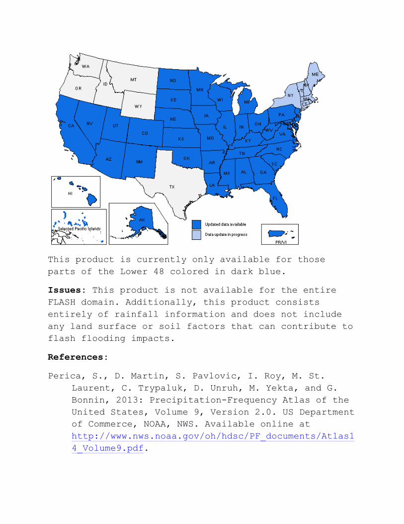
This is output from the FLASH web interface showing the 1-hr Precipitation Accumulation Return Period between 00 UTC and 01 UTC 4 Sept 2013 on the west and south sides of the Denver, Colorado metropolitan area. The maximum return period is outlined in the dark purple pixels and corresponds to a one-hour rainfall return period of 100 years or more.
This product is currently only available for those parts of the Lower 48 colored in dark blue.
Issues: This product is not available for the entire FLASH domain. Additionally, this product consists entirely of rainfall information and does not include any land surface or soil factors that can contribute to flash flooding impacts.
References:
Perica, S., D. Martin, S. Pavlovic, I. Roy, M. St. Laurent, C. Trypaluk, D. Unruh, M. Yekta, and G. Bonnin, 2013: Precipitation-Frequency Atlas of the United States, Volume 9, Version 2.0. US Department of Commerce, NOAA, NWS. Available online at http://www.nws.noaa.gov/oh/hdsc/PF_documents/Atlas14_Volume9.pdf.
Precipitation-to-Flash Flood
Guidance Ratio (QPE-to-FFG Ratio)
Short Description: Ratio of 1-, 3-, or 6-hr radar precipitation estimate to the corresponding 1-, 3-, or 6-hr flash flood guidance grid
Long Description: Clark et al. (2014) describe the state of the NWS flash flood guidance program across the United States. Several methods for producing FFG have been developed at the regional River Forecast Center level. This product relies on the standard FFG grids produced by the RFCs and issued every 6-, 12-, or
24-hours. Intermediate FFG updates requested by WFOs or individual FFG modifications made at the WFO level will not be reflected in this product. The NCEP Weather Prediction Center mosaics the various RFC grids together to create a national grid. This national grid, updated at most every 6 hours, is compared to radar-only precipitation estimate grids from the MRMS system. Updates to the precipitation grids are available every 2 minutes and so updates to the ratio product are available every 2 minutes, as well.
Applications: QPE-to-FFG ratio can be used to identify specific areas where flash flood guidance is suggesting bankfull conditions on small natural stream networks.
Example Images:
This is an image from the FLASH web interface showing the 1-hour QPE to FFG ratio for the Denver metropolitan area at 01 UTC on 4 Sept 2013. Pixels in yellow indicate those areas where the 1-hr QPE is exceeding the 1-hr FFG.
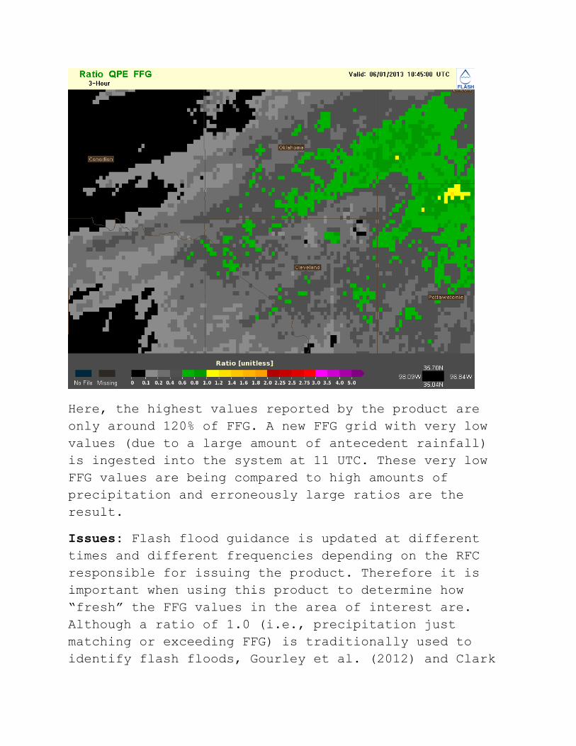
This is the 3-hr precipitation to FFG ratio for the Oklahoma City area valid at 11 UTC on 1 Jun 2013. This example illustrates the difficulties in using this product immediately after a new FFG product has been issued by an RFC. In the center of this image, the darkest purple pixels represent areas where precipitation is exceeding FFG by over 800%. Below is another image showing the same product valid 15 minutes earlier.
Here, the highest values reported by the product are only around 120% of FFG. A new FFG grid with very low values (due to a large amount of antecedent rainfall) is ingested into the system at 11 UTC. These very low FFG values are being compared to high amounts of precipitation and erroneously large ratios are the result.
Issues: Flash flood guidance is updated at different times and different frequencies depending on the RFC responsible for issuing the product. Therefore it is important when using this product to determine how “fresh” the FFG values in the area of interest are. Although a ratio of 1.0 (i.e., precipitation just matching or exceeding FFG) is traditionally used to identify flash floods, Gourley et al. (2012) and Clark
et al. (2014) determined that the product is nominally more skillful at a ratio of 1.5. Different methods are used to produce FFG, depending on the RFC. Therefore, in WFOs that have territory within two RFCs, FFG may be produced using different formulae. Use of the product immediately after updated FFG values are available can result in erroneously high QPE-to-FFG ratios.
References:
Clark III, R., J. J. Gourley, Z. Flamig, Y. Hong, and E. Clark, 2014: CONUS-wide evaluation of National Weather Service flash flood guidance products, Wea. Forecasting doi: 10.1175/10.1175/WAF-D-12-00124.1 (in press)
Gourley, J. J., J. Erlingis, Y. Hong, and E. Wells, 2012: Evaluation of tools used for monitoring and forecasting flash floods in the United States. Wea. Forecasting, 27, 158-173.
Observed Precipitable Water
(PW) Short Description: Precipitable water (PW) analysis over the continental United States (CONUS) derived from observed PW from atmospheric soundings (available at 00- and 12-UTC) Alternate Names: PW, precipitable water vapor Keywords: hydrometeorology, flash flood, FLASH Spatial Resolution: 0.01 x 0.01 deg Temporal Resolution: 12 hours Input Sources: observed soundings Availability: Q2FY16 (v11) Users: NWS WFOs, NWS RFCs, NWS NCEP WPC Long Description: As defined in the American Meteorological Society’s Glossary of Meteorology (2013), PW is “the total atmospheric water vapor contained in a vertical column of unit cross-sectional area extending between any two specified levels.” This metric is usually measured in terms of the height that the water would reach if it were completely condensed in a vessel the same shape as the column. PW is measured between the earth’s surface and 500 mb. In a study exploring the relationship between precipitable water, saturation thickness, and precipitation, Lowry (1972) pointed out that precipitable water decreases as station elevation increases. Equations used to calculate precipitable water can be found in Bolton (1980). Applications: PW can be used to determine heavy rainfall potential. Heavy rainfall and subsequent flooding may be more likely to occur when PW is greater than twice the climatological value for a geographic region. Example Images:
This image shows FLASH’s visualization of precipitable water (PW) based on observed soundings at 00:00 UTC on 21 July 2013. Each color band represents a certain amount of precipitable water, measured in inches. The higher the PW values, the greater the potential for heavy rainfall and flash flooding. Issues: It would be incorrect to use PW to predict heavy precipitation alone; while it is a measure of potential, it is only correctly interpreted when viewed in combination with regional climatology. In addition, as suggested by the NWS WFO in Rapid City, SD (2013), users of this plot should take care when interpreting these values due to uncertainty in interpolated data. References: American Meteorological Society, cited 2013:
“Precipitable Water.” Glossary of Meteorology. [Available online at http://glossary.ametsoc.org/wiki/Precipitable_water]
Bolton, D. 1980: The computation of equivalent potential temperature. Monthly Weather Review, 108, 1046-1053.
Lowry, D. A. 1972: Climatological relationships among precipitable water, thickness and precipitation. J. Appl. Meteor., 11, 1326-1333.
National Weather Service Weather Forecast Rapid City SD, cited 2014: “Upper-Air Climatology Plots.” [Available online at http://www.crh.noaa.gov/unr/?n=pw]
Observed Precipitable Water Percentile(PW Percentile) Short Description: Precipitable water percentile (PW Percentile) analysis over the continental United States (CONUS) derived from observed PW from atmospheric soundings and regional climatology (available at 00- and 12-UTC) Alternate Names: PW Anomaly, total precipitable water anomaly, PW Percentile Keywords: hydrometeorology, flash flood, FLASH, precipitable water, PW Spatial Resolution: 0.01 x 0.01 deg Temporal Resolution: 12 hours Input Sources: observed soundings Availability: Q2FY16 (v11) Users: NWS WFOs, NWS RFCs, NWS NCEP WPC Long Description: Precipitable water percentile refers to the magnitude of precipitable water measurements in comparison to climatological values for a given region. Across the CONUS, climatology data is sourced from a base map containing data from 1948-2013 (National Weather Service Weather Forecast Office Rapid City SD, 2014). PW percentile can be used in flash flood forecasting to indicate anomalies in levels of precipitable water, which may be connected to the potential for heavy rainfall and subsequent flash flooding. Applications: PW percentile is used in flash flood forecasting to identify regions that may have anomalous levels of atmospheric precipitable water. Heavy rainfall and subsequent flooding may be more likely to occur when PW percentile is greater than twice the climatological value for a geographic region. Example Images:
This image depicts a map of precipitable water percentiles across the CONUS on 21 July 2013 at 00:00 UTC. Issues: It would be incorrect to use PW Percentile to predict heavy precipitation alone; it is a measure of the potential for heavy precipitation. In the case shown above, there is great potential for heavy rainfall, but other ingredients (lift and instability) are lacking to initiate storms. In addition, users of this plot should take care when interpreting these values due to uncertainty in interpolated data (National Weather Service Weather Forecast Office Rapid City SD, 2014). References: American Meteorological Society, cited 2013:
“Precipitable Water.” Glossary of Meteorology. [Available online at http://glossary.ametsoc.org/wiki/Precipitable_water]
Bolton, D. 1980: The computation of equivalent potential temperature. Monthly Weather Review, 108, 1046-1053.
Forsythe, J. M., J. B. Dodson, P. T. Partain, S. Q. Kidder, and T. H. Vonder Haar, 2011: How total precipitable water vapor anomalies relate to cloud vertical structure. J. Hydrometeor., 13, 709-721.
National Weather Service Weather Forecast Rapid City SD, cited 2014: “Upper-Air Climatology Plots.” [Available online at http://www.crh.noaa.gov/unr/?n=pw]
Rapid Refresh Precipitable Water(Precipitable Water RAP) Short Description: Precipitable water (PW) analysis over the continental United States (CONUS) derived from the Rapid Refresh (RAP) modeling system Alternate Names: PW, total precipitable water, PW RAP Keywords: hydrometeorology, flash flood, FLASH, precipitable water, PW, Rapid Refresh, RAP Spatial Resolution: 0.01 x 0.01 deg Temporal Resolution: 1 hour Input Sources: RAP Availability: Q2FY16 (v11) Users: NWS WFOs, NWS RFCs, NWS NCEP WPC Long Description: As defined in the American Meteorological Society’s Glossary of Meteorology (2013), PW is “the total atmospheric water vapor contained in a vertical column of unit cross-sectional area extending between any two specified levels.” This metric is usually measured in terms of the height that the water would reach if it were completely condensed in a vessel the same shape as the column. PW is measured between the earth’s surface and 500 mb. In a study exploring the relationship between precipitable water, saturation thickness, and precipitation, Lowry (1972) pointed out that precipitable water decreases as station elevation increases. Equations used to calculate precipitable water can be found in Bolton (1980). Instead of using observed soundings to calculate PW, the PW RAP employs data from the Rapid Refresh (RAP) modeling system, which supports hourly short-range model forecasts out to 18-hours. Applications: PW can be used to determine the potential for heavy rainfall. Heavy rainfall and subsequent flooding may be more likely to occur when PW is greater than twice the climatological value for a geographic region.
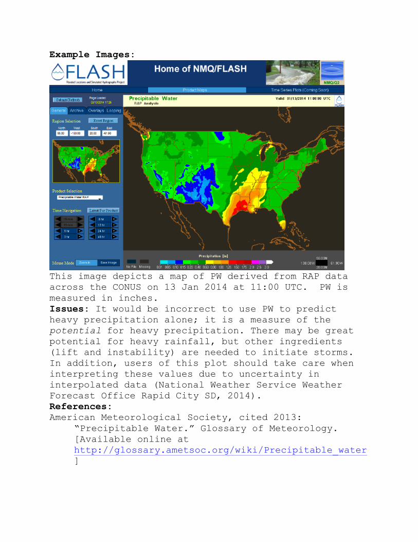
Example Images:
This image depicts a map of PW derived from RAP data across the CONUS on 13 Jan 2014 at 11:00 UTC. PW is measured in inches. Issues: It would be incorrect to use PW to predict heavy precipitation alone; it is a measure of the potential for heavy precipitation. There may be great potential for heavy rainfall, but other ingredients (lift and instability) are needed to initiate storms. In addition, users of this plot should take care when interpreting these values due to uncertainty in interpolated data (National Weather Service Weather Forecast Office Rapid City SD, 2014). References: American Meteorological Society, cited 2013:
“Precipitable Water.” Glossary of Meteorology. [Available online at http://glossary.ametsoc.org/wiki/Precipitable_water]
Bolton, D. 1980: The computation of equivalent potential temperature. Monthly Weather Review, 108, 1046-1053.
National Weather Service Weather Forecast Rapid City SD, cited 2014: “Upper-Air Climatology Plots.” [Available online at http://www.crh.noaa.gov/unr/?n=pw]
Rapid Refresh Precipitable Water Percentile (PW Percentile RAP) Short Description: Precipitable water percentile (PW Percentile) analysis over the continental United States (CONUS) derived from the Rapid Refresh (RAP) modeling system Alternate Names: RAP PW Anomaly, PW Percentile RAP Keywords: hydrometeorology, flash flood, FLASH, precipitable water, precipitable water percentile, PW percentile, Rapid Refresh, RAP Spatial Resolution: 0.01 x 0.01 deg Temporal Resolution: 1-hour Input Sources: RAP Availability: Q2FY16 (v11) Users: NWS WFOs, NWS RFCs, NWS NCEP WPC Long Description: Precipitable water percentile refers to the magnitude of precipitable water measurements in comparison to climatological values for a given region. Across the CONUS, climatology data is sourced from a base map containing data from 1948-2013 (National Weather Service Weather Forecast Office Rapid City SD, 2014). PW percentile can be used in flash flood forecasting to indicate anomalies in levels of precipitable water, which may be connected to heavy rainfall and subsequent flash flooding. Instead of using observed soundings to calculate PW, the PW RAP employs data from the Rapid Refresh (RAP) modeling system, which supports hourly short-range model forecasts out to 18-hours. Applications: PW percentile is used in flash flood forecasting to identify regions that may have anomalous levels of precipitable water. Heavy rainfall and subsequent flooding may be more likely to occur when PW percentile is greater than twice the climatological value for a geographic region.
Example Images:
This image depicts a map of precipitable water percentiles derived from RAP model data across the CONUS on 13 Jan 2014 at 11:00 UTC. Issues: It would be incorrect to use PW Percentile to heavy precipitation alone; it is a measure of the potential for heavy precipitation. In the case shown above, there is great potential for heavy rainfall, but other ingredients (lift and instability) are lacking to initiate storms. In addition, users of this plot should take care when interpreting these values due to uncertainty in interpolated data (National Weather Service Weather Forecast Office Rapid City SD, 2014). References: American Meteorological Society, cited 2013:
“Precipitable Water.” Glossary of Meteorology. [Available online at http://glossary.ametsoc.org/wiki/Precipitable_water]
Bolton, D. 1980: The computation of equivalent potential temperature. Monthly Weather Review, 108, 1046-1053.
Forsythe, J. M., J. B. Dodson, P. T. Partain, S. Q.
Kidder, and T. H. Vonder Haar, 2011: How total precipitable water vapor anomalies relate to cloud vertical structure. J. Hydrometeor., 13, 709-721.
National Weather Service Weather Forecast Rapid City SD, cited 2014: “Upper-Air Climatology Plots.” [Available online at http://www.crh.noaa.gov/unr/?n=pw]