Holding Patterns 101: Finding the Holy Grail of Timing and Wind Correction
Les Glatt, PhD. ATP/CFI-AI March 24, 2020
As part of the ACS requirements for an Instrument rating, the Pilot must
demonstrate an understanding and the required proficiency to fly a holding pattern. There are many training methods to provide the Pilot with the knowledge of how to visualize the holding pattern and enter the holding pattern. One of the required skills is IR.III.B.S5, which states, “Uses proper wind correction procedures to maintain the desired holding pattern, and to arrive at the holding fix as close as possible to a specified time”. The AIM provides some guidelines for estimating the outbound wind correction angle (OWCA), but there are no guidelines as under what conditions this rule-of-thumb should apply. In addition, there are no guidelines in the AIM for estimating the outbound time other than to fly a one-minute or one-minute and 30 second outbound leg for the initial circuit. The technique utilized to converge to the “Holding Pattern Solution” is based on a bracketing technique, which in reality is a “Trial and Error” method. Here we fly a specified OWCA and outbound time, and based on the inbound time and whether the aircraft has undershot/overshot the centerline of the inbound course, the Pilot will fly the next circuit with an updated outbound time and OWCA. The process continues until the Pilot converges to the correct “Holding Pattern Solution”. Depending on the initial guess for the outbound time and OWCA, the Pilot may require a significant number of circuits before converging to the correct holding pattern. This process of converging to the proper holding pattern can impose a considerable workload on the Pilot, especially when attempting to troubleshoot a problem, or while reviewing the approach plate prior to executing the approach.
Over the last fifty years there have been numerous articles, IFR training manuals, videos, blogs, and Pilot Forums that present techniques on how to compensate for the wind while flying the holding pattern. In 2018, a seminal paper was published on the holding pattern. The title of the paper is “A Treatise on the Holding Pattern: Expelling the Myths and Misconceptions of Timing and Wind Correction”. In this paper, this author derives the complete mathematical solution of the “Generalized Holding Pattern Problem”. Here the term “Generalized” refers to the holding pattern for which the aircraft flies an arbitrary constant turn rate, specifies an arbitrary inbound time or distance from the holding fix, and for any wind direction and wind speed up to the 99.99% of the TAS of the aircraft. The mathematics involved is based on elementary trigonometry, algebra and calculus. Because the solution is completely analytic, an enormous amount of information about the holding pattern can be deduced. It is the intent of this article to
summarize the results of this paper and show that over 90 percent of the material that has been presented in the past on the subject of timing and wind correction in the holding pattern has been both incorrect and misleading.
Figure 1 shows a non-standard holding pattern. We designate the point 0 as the holding fix. point 1 is the location of the aircraft at the completion of the outbound turn. point 2 is the location of the aircraft at the end of the outbound time, and point 3 is the location of the aircraft at the point the aircraft re-intercepts the inbound course at the time the aircraft heading is the inbound course plus the inbound wind correction angle (IWCA). Note that it is no longer necessary to determine the abeam point since the outbound time is measured from the point the aircraft reaches the required outbound heading. Thus, Pilot workload is reduced by not spending time locating the abeam point. In addition, the (x, y) location of the aircraft CG is normalized by the aircraft TAS in nm/sec, so by multiplying the (x, y) coordinates by the TAS, gives the actual extent of the holding pattern in nm.
Figure 1: Non-Standard Holding Pattern
The solution of the “Holding Pattern Problem” is shown to be a function of the following parameters:
(a) Windspeed ratio, , i.e. the ratio of the windspeed to the aircraft TAS (VTAS). (b) Wind angle, (deg) relative to the inbound course to the holding fix. (c) Aircraft rate of turn, (rad/sec) or k (deg/sec) (d) Required inbound time to the fix in minutes, , i.e. one-minute or one-minute
Although the shape of the holding pattern is a function of the above four parameters, the extent of the holding pattern (i.e. what the Radar Controller observes on the radar
scope) is also a function of the parameter , since the coordinates of the
holding pattern are proportional to this parameter.
The analysis in the paper provides 3 important equations that provide the Pilot with the outbound time the aircraft must be flown along the segment 1-2, the outbound heading the aircraft must fly along the segment 1-2, and the inbound wind correction angle. These equations are provided below for the interested reader.
(1)
(2)
Here, k is the turn rate in deg/sec, is the outbound heading relative to the inbound course, and is the inbound wind correction angle in degrees relative to the inbound course. The IWCA is given by
(3)
Here , and is the wind angle relative to the inbound course. Note that eq. (3)
is the result one obtains from solving the standard “Wind Triangle Problem”. In addition, a1-a3 is given by
(4)
The variable is the required inbound time to the fix in minutes, i.e. either one-minute below 14000MSL, or 1.5 minutes above 14000MSL. Thus, the entire solution to the “Generalized Holding Pattern Problem” is contained in eqs. (1)-(4).
In order to orient the reader, positive values of corresponds to a wind coming from the holding side, while negative values of corresponds to a wind coming from the non-holding side. Similarly, positive values of means the aircraft is crabbed toward the holding side, and negative values of means the aircraft is crabbed toward
the non-holding side. Once the values of k, , , VWIND, and VTAS are provided, the entire solution of the “Holding Pattern Problem” is determined exactly.
There is an interesting geometric property of the holding pattern when we compare the holding pattern for the case when the wind is blowing from the direction , and the wind blowing from the direction - . In this scenario, if the relative outbound heading for positive is , the relative outbound heading in the case of - is just - . This translates to the simple relationship OWCA ( )=-OWCA ( ). We designate the
OWCA ( ) as OWCA’. This is shown below in Figure 2, where we compare the case for which the Pilot is flying a non-standard holding pattern with a windspeed ratio
, with a 45-degree wind angle relative of the inbound course. The points 1’, 2’, and 3’ correspond to the degree case, whereas the points 1, 2, and 3, correspond to degree case. When , and . Thus, as a consequence of this geometric property, eq. (1) shows that if the outbound time is started when the aircraft has turned to the outbound heading, the inbound time is the same when (i.e. the same inbound time, whether flying left or right hand turns). The advantage of starting the outbound time when the aircraft has turned to the outbound heading, is the Pilot no longer needs to locate the abeam point, which reduces Pilot workload in the cockpit.
Figure 2: Geometric Property of the Holding Pattern
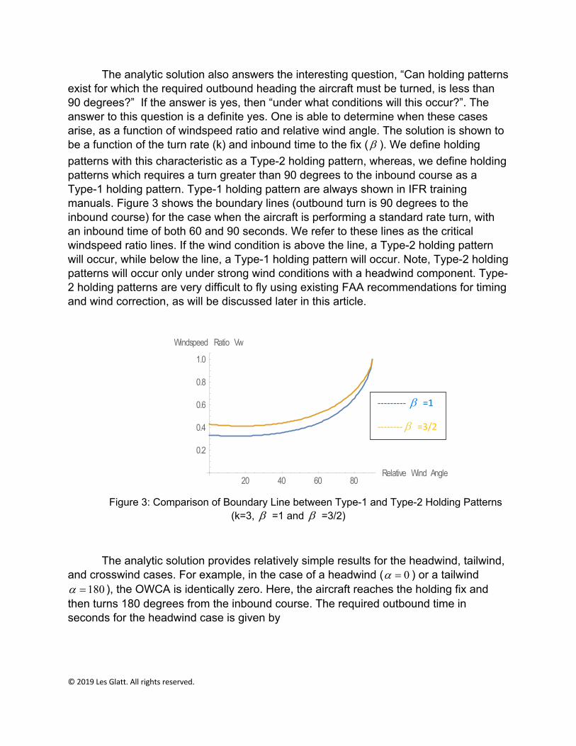
The analytic solution also answers the interesting question, “Can holding patterns exist for which the required outbound heading the aircraft must be turned, is less than 90 degrees?” If the answer is yes, then “under what conditions will this occur?”. The answer to this question is a definite yes. One is able to determine when these cases arise, as a function of windspeed ratio and relative wind angle. The solution is shown to be a function of the turn rate (k) and inbound time to the fix ( ). We define holding patterns with this characteristic as a Type-2 holding pattern, whereas, we define holding patterns which requires a turn greater than 90 degrees to the inbound course as a Type-1 holding pattern. Type-1 holding pattern are always shown in IFR training manuals. Figure 3 shows the boundary lines (outbound turn is 90 degrees to the inbound course) for the case when the aircraft is performing a standard rate turn, with an inbound time of both 60 and 90 seconds. We refer to these lines as the critical windspeed ratio lines. If the wind condition is above the line, a Type-2 holding pattern will occur, while below the line, a Type-1 holding pattern will occur. Note, Type-2 holding patterns will occur only under strong wind conditions with a headwind component. Type-2 holding patterns are very difficult to fly using existing FAA recommendations for timing and wind correction, as will be discussed later in this article.
Figure 3: Comparison of Boundary Line between Type-1 and Type-2 Holding Patterns (k=3, =1 and =3/2)
The analytic solution provides relatively simple results for the headwind, tailwind, and crosswind cases. For example, in the case of a headwind ( ) or a tailwind
), the OWCA is identically zero. Here, the aircraft reaches the holding fix and then turns 180 degrees from the inbound course. The required outbound time in seconds for the headwind case is given by
In the tailwind case, the outbound time in seconds is given by
(6)
In the case of a standard rate turn (k=3) with a one-minute inbound leg ( ), the outbound time in the headwind case becomes
(7)
And in the tailwind case, the outbound becomes
(8)
Figure 4 shows the track of the aircraft in the holding pattern corresponding to a windspeed ratio of 0.2. In the case of a standard rate turn and one-minute inbound leg, the outbound time in the headwind case is 20 seconds and in the tailwind case the outbound time is 120 seconds.
Figure 4: Non-Standard Holding Pattern: Headwind and Tails Cases for =0.2
Equation (7) shows that the outbound time goes to zero when the windspeed
ratio is exactly . The case of tout=0 corresponds to a holding pattern in which the
aircraft reaches the holding fix and then executes a 360 degree turn to re-intercept the inbound course. The aircraft then flies one-minute to reach the fix. The total time for one circuit of the holding pattern is exactly 3 minutes. Figure 5 shows this type of holding pattern.
One would surmise that when the windspeed ratio is greater than , the Pilot
would not be able to satisfy the one-minute inbound requirement. This requirement could only be satisfied if the aircraft tracks the outbound radial from the fix for a specified time. Since in this case the aircraft does not turn after reaching the fix, the analytic solution provides the outbound time beyond the fix as
If the Pilot knows , it is possible to determine the required outbound time using
the following method: When the aircraft reaches the holding fix, the Pilot performs a 360-degree turn and then determines the inbound time to the fix. The difference between the inbound time and the required one-minute inbound time is determined. This time difference is the time required to fly beyond the holding fix along the outbound course.
In the crosswind case, the analytic solution provides the following equations for the relative outbound heading and outbound time for the case k=3 and . Again, the relative outbound heading is just the number of degrees the aircraft must be turned relative to the inbound course.
(10)
(11)
Figure 6 shows the track of the holding pattern for windspeed ratios of 0.1, 0.2 and 0.3. In this case, the aircraft is flying a non-standard holding pattern with the inbound course being 360 degrees and the wind coming from 270 degrees. Each depicted holding pattern is annotated with the IWCA, OWCA, and outbound time. The FAA recommends using an initial estimate for the OWCA being 3 times the IWCA. One can define the M-Factor as the ratio of the OWCA to the IWCA. As can be seen in Figure 6, the M-Factor is 2.96 for 0.1, 2.86 for 0.2, and 2.70 for 0.3. The corresponding outbound times are 62.4 seconds, 70 seconds, and 83.7 seconds. Based on the crosswind case, one may conclude that using a value of 3 for the M-Factor should provide a valid estimate for the OWCA under most windspeed ratios and relative wind angles and thus be consistent with the FAA recommendation for estimating the OWCA.
As we shall soon see, this assumption is far from being correct.
Figure 6: Non-Standard Holding Pattern: Direct Crosswind with 0.1, 0.2, and 0.3
Most Pilots will fly Type-1 holding patterns in the majority of the holding patterns they fly. We will now show the required IWCA, M-Factor, and required outbound time, for windspeed ratios 0.05, 0.1, 0.15, 0.2, 0.25, and 0.3 for Type-1 holding patterns typically flown by GA aircraft (i.e. below 14000MSL and k=3). Figure 7 shows the IWCA as a function of the relative wind angle for the above windspeed ratios.
Figure 7: Magnitude of the IWCA versus Relative Wind Angle for Values of
Note the IWCA is symmetric around the 90-degree relative wind angle, as well as having its maximum value at the 90-degree relative wind angle. This means that the IWCA is double-valued, with one value corresponding to a headwind component, and one corresponding to the tailwind component. Thus, if the Pilot has found the IWCA to track the inbound course, it will be necessary to use groundspeed information to determine whether the relative wind angle is less than or greater than 90 degrees. A simple rule-of-thumb for windspeed ratios less than 0.5 is the maximum value of the IWCA is given by
(12)
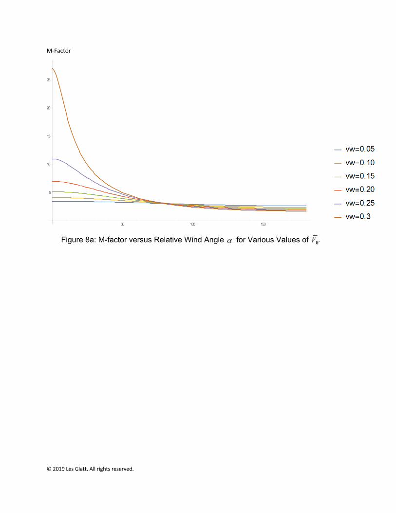
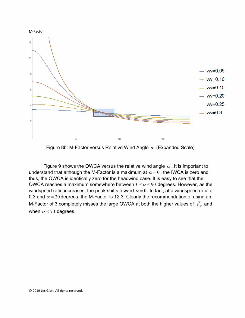
Figure 8a shows the corresponding value of the M-Factor as a function of the relative wind angle and the windspeed ratio. In Figure 8b we have drawn a cyan box corresponding to the bounds for the M-Factor between 2.5 and 3.5. This region is consistent with the FAA recommendation of using a value of 3 for the M-Factor. The analysis shows the value of 3 is valid for all relative wind angles, when the windspeed ratio less than 0.05. For windspeed ratios up to 0.3, the relative wind angle is limited to between 70 and 95 degrees. In Figure 8a, the maximum value of the M-Factor occurs on a direct headwind ( ) and the minimum value occurs on a direct tailwind (
). The exact solution shows that the bounds on the M-Factor are given by the following inequality
(13)
The bounds on the M-Factor in eq. (13) completely debunk the statements in IFR training manuals and published articles that the “M-Factor is always between 2 and 3”.
In the weak wind limit, where the windspeed ratio approaches zero, the limiting value of the M-Factor is given by
(M-Factor) (14)
Note, the weak wind limiting value is only a function of the product . Equation (14) is extremely important because it tells the Pilot that the M-Factor is not that same for all types of holding patterns. For example, in the case of a GA aircraft in a holding pattern with a one-minute inbound time and using a standard rate turn, the limiting multiplier is
3. However, if that same aircraft holds above 14000MSL, where , the limiting
multiplier is 2.33. Next, consider a commercial jet flying above 14000MSL in a holding pattern. The rate of turn at the holding speed will most likely be limited to a 25-degree bank while using the flight director. The equation for the rate of turn of the aircraft is given by
(15)
where g is the acceleration of gravity (32.17 ft/sec^2), the bank angle, and the VTAS is the TAS in feet/sec. In order to convert knots to feet/sec, we multiply the TAS in knots by 1.6875. If the aircraft is holding at 20000MSL (i.e. FL200) at about 260 KIAS, the rate of turn will be about half-standard rate, i.e.1.5 deg/sec. Under these conditions, with a 90-second inbound time to the fix, the limiting value of the M-Factor will be approximately 3.67. Thus, the limiting weak wind multiplier will not be a constant and will vary depending on the type of holding pattern flown.
Although we have discussed inbound time to the fix, any requirement for intercepting the inbound course at a fixed distance from the holding fix can be recast as an inbound time constraint, where the inbound time is determined by dividing the required distance from the fix by the groundspeed along the inbound course to the fix. This allows the exact solution of the “Holding Pattern Problem” to be utilized with both an inbound time constraint or distance constraint. For example, if the required inbound distance from the fix is LIC, then the required inbound time to the fix, , is given by
(16)
Here, VTAS is in nm/sec.
Equation (13), with k=3 and , provides an important piece of information that every IFR Pilot should understand. As the windspeed ratio increases, for cases with a headwind component, the M-Factor will always be bounded by
(17)
Similarly, with a tailwind component, the M-Factor will always be bounded by
(18)
Therefore, in the tailwind case, as the windspeed ratio approaches 1, the M-Factor approaches unity. Thus, the M-Factor with a tailwind component will always be bounded
between 1 and 3. Whereas, in the case of a headwind component, the bound on the M-Factor is given by eq. (17). When the windspeed ratio is 0.3, the bound on the M-Factor in the case of a headwind component is between 3 and 27. This is a considerably larger bound than in the tailwind case, where the bound is between 1 and 3. Thus, as the windspeed ratio increases, any bracketing technique used to converge to the correct holding pattern will always require more circuits with a headwind component than with a tailwind component. For example, in the case of a tailwind component, if the winds are not light, the Pilot can always start with an M-Factor of 2. Depending on the result of the overshoot or undershoot of the inbound course, the next circuit the Pilot could use an M-Factor of either 1.5 or 2.5. We see that the upper and lower bounds converge relatively quickly. If the windspeed ratio was 0.3, in the case of a headwind component, there is a large difference between the upper and lower bound and the Pilot would require a significant number of circuits to bracket the holding pattern solution.
Figure 8b: M-Factor versus Relative Wind Angle (Expanded Scale)
Figure 9 shows the OWCA versus the relative wind angle . It is important to understand that although the M-Factor is a maximum at , the IWCA is zero and thus, the OWCA is identically zero for the headwind case. It is easy to see that the OWCA reaches a maximum somewhere between degrees. However, as the windspeed ratio increases, the peak shifts toward . In fact, at a windspeed ratio of 0.3 and degrees, the M-Factor is 12.3. Clearly the recommendation of using an M-Factor of 3 completely misses the large OWCA at both the higher values of and when degrees.
Figure 9: OWCA versus Relative Wind Angle for Various Values of
In order to understand why the M-Factor is smaller with a tailwind component than with a headwind component, we show the holding pattern case for a windspeed ratio of 0.3 with the relative wind angles of 45 degrees and 135 degrees. The 45-degree case has a headwind component and the 135 has a tailwind component. Figure 10 shows the comparison between the two cases. Note the significant difference in the OWCA between the two cases. In the case of a tailwind component on the inbound course, the aircraft must be flown further outbound in order to meet the required one-minute inbound leg. In order to prevent the aircraft from undershooting the inbound course, the OWCA must be smaller. Since the IWCA will be the same in both cases, it can easily be seen that the M-Factor in the tailwind case will be smaller than in the headwind case. However, in the weak wind limit, the M-Factor is independent of the relative wind angle.
Figure 10: Comparison of M-Factor for , and degrees
In regard to timing of the outbound leg in the presence of a wind, the latest AIM states that the initial outbound leg should be flown for either 60 or 90 seconds, depending on the aircraft altitude, and for subsequent circuits, the outbound time should be adjusted as necessary to achieve the appropriate inbound time or distance from the holding fix. The FAA does not provide a rule-of-thumb on how to correct the outbound time for future circuits. However, in the AOPA Pilot’s Manual for Instrument Flying (Thom, 1990), the author provides two rules-of-thumb for correcting the outbound time. In the case of strong headwinds or tailwinds, the author suggests that the outbound time should be corrected by 2 seconds per knot. Thus, when flying inbound on a headwind, the outbound time should be reduced by 2 seconds per knot of wind, and when flying inbound on a tailwind, the outbound time should be increased by 2 seconds per knot of wind. In a second rule-of-thumb, the author recommends that the Pilot double the error of the inbound time deviation. For example, if the inbound time is 45 seconds, on the next circuit, the outbound time should be increased by 30 seconds. Conversely, if the inbound leg required 70 seconds, the outbound time for the next circuit should be reduced by 20 seconds. Again, these rules-of-thumb do not come with any limitations under which they provide reasonable results.
The analytic solution of the holding pattern provides the outbound time from the point the aircraft has turned to the outbound heading. Figure 11 below, shows the
outbound time as a function of the relative wind angle for windspeed ratios 0.05, 0.1, 0.15, 0.2, 0.25, and 0.3.
tOUT (sec)
Relative Wind Angle (degrees)
Figure 11: Required Outbound Time versus Relative Wind Angle
for Various Values of
Note, the relative spacing between the curves of constant windspeed ratio are not constant. It is easy to see the difference between two consecutive windspeed ratio curves on the headwind and tailwind are different, with the headwind ( ) having a smaller spacing than the tailwind ( ) between the two consecutive curves. However, the change in windspeed ratio between the two curves is the change in windspeed divided the VTAS. The analytic solution allows one to determine the gradient of the outbound time with respect to the windspeed (i.e. the change in required outbound time for a given change in windspeed). The outbound time gradients are shown below for the cases for which the aircraft is on a headwind while flying inbound to the fix (HW), or a tailwind while inbound to the fix (TW), i.e.
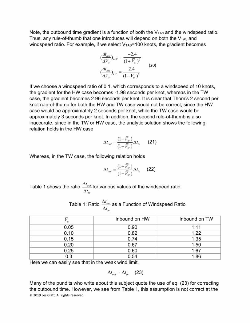
Note, the outbound time gradient is a function of both the VTAS and the windspeed ratio. Thus, any rule-of-thumb that one introduces will depend on both the VTAS and windspeed ratio. For example, if we select VTAS=100 knots, the gradient becomes
(20)
If we choose a windspeed ratio of 0.1, which corresponds to a windspeed of 10 knots, the gradient for the HW case becomes -1.98 seconds per knot, whereas in the TW case, the gradient becomes 2.96 seconds per knot. It is clear that Thom’s 2 second per knot rule-of-thumb for both the HW and TW case would not be correct, since the HW case would be approximately 2 seconds per knot, while the TW case would be approximately 3 seconds per knot. In addition, the second rule-of-thumb is also inaccurate, since in the TW or HW case, the analytic solution shows the following relation holds in the HW case
(21)
Whereas, in the TW case, the following relation holds
(22)
Table 1 shows the ratio for various values of the windspeed ratio.
Here we can easily see that in the weak wind limit,
(23)
Many of the pundits who write about this subject quote the use of eq. (23) for correcting the outbound time. However, we see from Table 1, this assumption is not correct at the
higher windspeed ratios. In fact, the ratio in the case of a headwind on the inbound leg is the inverse of the ratio in the case of a tailwind on the inbound leg. This result debunks Thom’s second rule-of-thumb for correcting the outbound time.
Finally, in the crosswind case, the outbound time gradient is given by
(24)
If we substitute VTAS=100 knots in eq. (24), we obtain the result
(25)
If we assume a windspeed ratio of 0.1, the outbound time gradient is approximately 0.5 seconds per knot, far different than the 2 and 3 second per knot for the HW and TW cases. Thus, one can easily see that attempting to provide a simple rule-of-thumb for outbound time corrections for all the possible holding pattern scenarios is just not possible. This is an important take-away for all IFR Pilots to understand.
We now turn our attention to Type-2 holding patterns. Type-2 holding patterns have never been documented in the open literature. As discussed earlier, the Type-2 holding pattern will occur while holding on a strong headwind component. Again, Figure 3 shows the boundary line for the critical windspeed ratio versus . We see in the case of a windspeed ratio of 0.4 with a relative wind coming from 30 degrees on the holding side will produce a Type-2 holding pattern. Figure 12 shows the solution of a non-standard holding pattern with a 360- degree inbound course and the wind coming from 330 degrees. In this case the required outbound heading to fly is 297 degrees (OWCA equal to 117 degrees), whereas the IWCA is approximately 12 degrees. The required outbound time between point 1 and 2 is approximately 35 seconds. The first interesting observation about this holding pattern is the definite lack of the ability of the Pilot to locate the abeam point. Thus, the Pilot would need to start the outbound time at point 1. Note, this is a recommendation in the AIM when the abeam point cannot be determined. The shape of the holding pattern is significantly different than the Type-1 holding pattern most IFR Pilots are taught during their training for the instrument rating. In addition, when attempting to converge to this holding pattern solution, the overshoot/undershoot of the inbound course is controlled by the outbound time, whereas, the inbound time is controlled by the outbound heading. This is opposite to the way IFR Pilots are trained in correcting for timing and wind correction for Type-1 holding patterns.
Type-2 holding patterns still have the same geometric property when the relative wind angle is the same, except coming from the non-holding side (wind direction 030 degrees). We see this in Figure 13 where we have compared the two non-standard holding patterns corresponding to a windspeed ratio of 0.4 and wind directions from 330 and 030 degrees. Here, points 1, 2 and 3 correspond to the wind coming from 330 degrees, and points 1’, 2’, and 3’ correspond to the wind coming from 030 degrees. Note the outbound time between points 1 and 2 is identical to the outbound time between points 1’ and 2’. However, in the case of the wind direction 030 degrees, one can identify the abeam point. It is easy to see that if the Pilot started his outbound time from the abeam point, the outbound time will be considerably longer than the outbound time between points 1’ and 2’. However, for all holding patterns flown, it is better to always start the outbound time at points 1 and 1’. In addition, the OWCA for the wind 030 is just the negative of the OWCA for the 330-degree case, which again, is the general geometric property of any holding pattern.
Figure 13: Comparison of Type-2 Non-Standard Holding Pattern
(Windspeed Ratio=0.4, Wind Direction 330 and 030 deg)
Now that we have shown the actual complexity of flying the holding pattern when the windspeed ratio is greater than about 0.05, we will delve into the FAA recommended technique used to converge to the “Holding Pattern Solution”, and show that as the windspeed increases, the method is very inefficient in converging to the correct holding pattern. We will start with flying Type-1 holding patterns. We showed earlier that the AIM recommendation is to start with an OWCA that is three times the IWCA and an outbound time of 60 seconds. Based on the results of the first circuit, the Pilot estimates both the change in the OWCA and the outbound time in order to intercept the inbound course with the proper inbound time or distance from the holding fix. If the inbound time is less than the required inbound time, the Pilot will increase the outbound time. If the aircraft overshoots the inbound course, the Pilot will increase the OWCA, and if the aircraft undershoots the inbound course, the Pilot will decrease the OWCA. This simple rule was expected to allow the Pilot to converge to the correct “Holding Pattern Solution” in a minimum number of circuits. However, the number of circuits required to arrive at the correct answer depends on two factors. First, how close the initial guess for holding pattern is compared to the exact solution for the holding pattern; and second, the method used to converge to the correct “Holding Pattern Solution”.
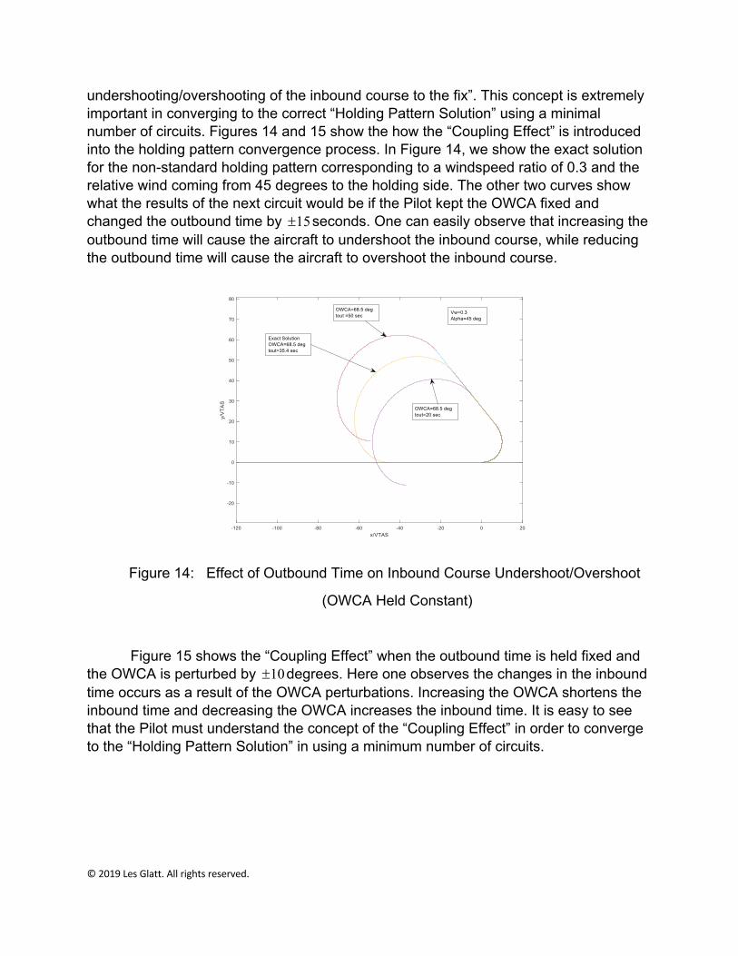
There is one characteristic of the bracketing technique that is never discussed in any FAA or IFR training manuals. This characteristic is called the “Coupling Effect”. The concept of the “Coupling Effect”, which states that “Every Pilot induced change in the outbound time or OWCA causes changes in both the inbound time and the
undershooting/overshooting of the inbound course to the fix”. This concept is extremely important in converging to the correct “Holding Pattern Solution” using a minimal number of circuits. Figures 14 and 15 show the how the “Coupling Effect” is introduced into the holding pattern convergence process. In Figure 14, we show the exact solution for the non-standard holding pattern corresponding to a windspeed ratio of 0.3 and the relative wind coming from 45 degrees to the holding side. The other two curves show what the results of the next circuit would be if the Pilot kept the OWCA fixed and changed the outbound time by seconds. One can easily observe that increasing the outbound time will cause the aircraft to undershoot the inbound course, while reducing the outbound time will cause the aircraft to overshoot the inbound course.
Figure 14: Effect of Outbound Time on Inbound Course Undershoot/Overshoot
(OWCA Held Constant)
Figure 15 shows the “Coupling Effect” when the outbound time is held fixed and the OWCA is perturbed by degrees. Here one observes the changes in the inbound time occurs as a result of the OWCA perturbations. Increasing the OWCA shortens the inbound time and decreasing the OWCA increases the inbound time. It is easy to see that the Pilot must understand the concept of the “Coupling Effect” in order to converge to the “Holding Pattern Solution” in using a minimum number of circuits.
Figure15: Effect of OWCA on Inbound Time (tout Held Constant)
Using the exact solution of the “Holding Pattern Problem”, a “Smart-Convergence” algorithm for Type-1 holding patterns was developed in order to converge to the correct holding pattern in a minimum number of circuits. This algorithm is compared to the current bracketing technique, and shows there are significant deficiencies in the “Bracketing Method” that require additional circuits to converge to the correct holding pattern. Table 2 shows the correct Pilot response in converging to the “Holding Pattern Solution”. The rows correspond to the inbound time. If the inbound time is less than the required inbound time, the row is defined as dx<0. If the inbound time is greater than the required inbound time, the row is defined as dx>0. If the inbound time matches the required inbound time the row is defined as dx=0. In regard to the overshoot/undershoot of the inbound course, if the aircraft overshoots the inbound course, the column is defined as dy>0. If the aircraft undershoots the inbound course, the column is defined as dy<0, and if the aircraft intercepts the inbound course the column is defined as dy=0. Note that all entries in “Green” are those required by the bracketing technique, and agree with the “Smart-Convergence Algorithm”. Entries in “Cyan” and “Red” are those corrections which are due to the “Coupling Effect”. The Cyan entries are required by the “Smart-Convergence” algorithm. In addition, all entries in “Red” are those required by both the bracketing technique and the “Smart-Convergence” algorithm. The “?” symbol following the Red entry indicates the direction of this correction can only be determined using the “Smart-Convergence Algorithm”. This means the actual values of dx and dy from the previous circuit must be used to determine which direction the correction must be made. It is impossible for the Pilot to do this type of mental arithmetic while flying the aircraft. As the windspeed ratio picks up, the “Coupling Effect” becomes stronger, and thus the number of circuits to converge
to the correct holding pattern increase, making the “Bracketing Method” very inefficient and causes the Pilot workload to increase considerably.
Table 2: Comparison of Corrective Actions between Bracketing Method and Smart-Convergence Tool Algorithm
Undershoot (dy<0) On Course (dy=0) Overshoot (dy>0)
Inbound Time Early (dx<0) Increase tout? Decrease OWCA
Increase tout Decrease OWCA
Increase tout Increase OWCA?
On Time (dx=0) Decrease tout Decrease OWCA
No Change in both tout and OWCA
Increase tout Increase OWCA
Inbound Time Late (dx>0) Decrease tout Decrease OWCA?
Decrease tout Increase OWCA
Decrease tout? Increase OWCA
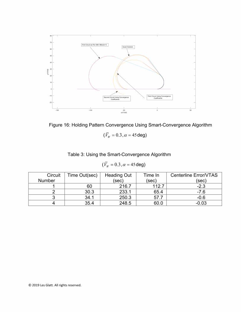
We will use the example of a non-standard holding pattern with the inbound course being 360 degrees, the windspeed ratio equal to 0.3, and the relative wind angle equal to 45 degrees from the holding side (i.e. a wind direction of 315 degrees). Figure 16 shows the aircraft track of each consecutive holding pattern. The first circuit is always flown as recommended by the AIM. Table 3 shows the outbound time, outbound heading, inbound time, and inbound course overshoot/undershoot error of each of the consecutive circuits during the convergence process. We can compare these tracks with the exact solution of the holding pattern. We see that the holding pattern is very close to convergence by the third circuit, and completely converged by the fourth circuit.
Figure 17 shows the holding pattern tracks during the convergence process using the standard bracketing technique based on an average IFR Pilot flying the aircraft. Note, by the fifth circuit, the holding pattern is close to being converged, whereas, the Smart-Convergence algorithm is very close to being converged after three circuits. The additional circuits required in the bracketing technique is due the Pilot not accounting for the “Coupling Effect” during the convergence process. Table 4 shows the resultant outbound time, outbound heading, inbound time, and overshoot/undershoot error for the consecutive circuits during the convergence process.
We have seen that the non-optimal convergence process of the bracketing technique arises because of the Pilot trying to converge the holding pattern with two unknown parameters (OWCA and outbound time). One can reduce the number of circuits by specifying one of the variables and converging on the second. Consider the case of the Pilot eyeballing the outbound time from Figure 11. If we take the outbound time as 35 seconds, then, for all future circuits, the aircraft is flown with different OWCA and a 35 second outbound time. Figure 18 shows the aircraft track in the consecutive circuits. The first circuit uses the AIM recommendation of three times the IWCA. The second circuit increases the OWCA by 20 degrees to correct for the overshoot. The third circuit increases the OWCA by 10 degrees to again correct for the overshoot on
the second circuit. Note, after three circuits the holding pattern is essentially converged to the exact solution. Table 5 shows the outbound heading, outbound time, inbound time, and the overshoot/undershoot error for each consecutive circuit. The rapid convergence is due to the elimination of the “Coupling Effect”, and converging on a single variable, the OWCA.
Figure 18: Eyeballing Outbound Time from Figure 11
Average IFR Pilot Estimating OWCA)
Table 5: Convergence History of Holding Pattern by Eyeballing tout from Figure 11
Flying the Type-2 holding pattern is definitely a challenge for any IFR Pilot. Over 99% of IFR Pilot population would be frustrated attempting to converge to this holding pattern. Figure 19 shows a comparison of the holding pattern shown in Figure 12 with the first circuit flown using the FAA recommendation, i.e. three times the IWCA with 60 second outbound time. Note the extreme difference between the initial guess and the correct holding pattern shape. The inbound time after the first circuit is over 176 seconds. There are no guidelines in how to fly Type-2 holding patterns. Note the
outbound turn is approximately 63 degrees from the inbound course. In this holding pattern, the outbound time controls the undershoot/overshoot of the inbound course, while the outbound heading controls the inbound time. In addition, the correct holding pattern does not contain an abeam point for the outbound time to start. It is doubtful that without the knowledge of the existence of the Type-2 holding pattern, nearly all IFR Pilot’s would spend a considerable amount of time trying to get to the final pattern, and a significant number would just give up.
Comparison of Exact Solution with AIM Recommendations for First Circuit
The exact solution of the “Holding Pattern Problem” provides another important capability which relates to IFR flying. When an IFR pilot receives a holding clearance, one important piece of information that should be given by ATC is either an EFC (expect further clearance time) or an EAC (expect approach clearance time). This time is important since it allows the Pilot to know when he/she is expected to leave the holding fix. ATC can amend the EFC or EAC at any time, however, in the event of lost communications in IFR conditions, the Pilot is expected to leave the holding fix at that time. The “Holding Pattern Solution”, provides the Pilot with the outbound heading and outbound time in order to satisfy the 60/90-second required inbound time, or the required inbound distance from the fix. When one is interested in reaching the fix exactly at the EFC or EAC time, the final holding pattern may have to be adjusted in order to leave the fix at the correct time. This adjustment manifests itself by determining a new outbound heading and outbound time to satisfy the EFC/EAC time. For example, under a no-wind condition, the total time for the holding pattern with a one-minute inbound leg would be 4 minutes. Consider the case where the EFC/EAC is 20 minutes from the time the Pilot accepts the holding clearance. If the Pilot crosses the fix and
initiates the outbound turn 5 minutes later, the remaining time in the holding would be 15 minutes. Under these conditions, the Pilot would fly 3 holding patterns and have 3 minutes remaining to return to the fix. In this case the Pilot could shorten the outbound leg by 30 seconds and reach the holding fix exactly at the EFC/EAC time. However, in the case of an arbitrary windspeed and wind direction, the Pilot will need to guess how to modify these parameters. Below we describe an example of a situation involving an EFC/EAC time where the analysis provides the required information to the Pilot.
The Pilot receives the following clearance from ATC: “N1234 is cleared direct to XYZ. Hold south on the 180-radial, left turns, maintain 5000 thousand. Expect further clearance at 1325. Time now 1300”. After repeating the clearance back to ATC, the aircraft proceeds direct to XYZ and enters the hold. After intercepting the 180-radial, the aircraft flies inbound and crosses XYZ. The Pilot notes the time crossing XYZ is 1309. The aircraft has 16 minutes to arrive back at XYZ in order to depart the fix at 1325. We will assume the aircraft is flying at a TAS of 100 knots, and the wind speed is 40 knots coming from 330 degrees magnetic. This holding pattern corresponds to the case shown in Figure 12. The total time for one complete circuit of this holding pattern is 3 minutes and 35 seconds. If the Pilot flies 4 complete circuits, the aircraft will arrive at XYZ after 14 minutes and 20 seconds, which is one-minute and 40-seconds early. However, if the pilot flies 3 complete circuits, the Pilot will have 5 minutes and 15 seconds remaining to get back to XYZ in order to depart the fix at the EFC time. Since the Pilot knows the total time for the next complete circuit (i.e. 315 seconds), the analysis determines the new inbound time, , for the final circuit. In this situation, we determine the required inbound time to be 147 seconds. Using eq. (1), we determine the outbound time to be 48 seconds. Thus, in order to satisfy the EFC/EAC time back at the holding fix, we need to increase the outbound time by 13 seconds. Under these conditions, the inbound time will increase by 87 seconds. Since the inbound time is significantly larger than the normal one-minute required inbound time for the holding pattern, the critical windspeed ratio will increase to 0.53. This is higher than the existing windspeed ratio of 0.4, and thus, the final holding pattern reverts back to a Type-1 holding pattern. Here the Type-1 holding pattern requires an outbound heading of 224 degrees, whereas, the Type-2 holding pattern that was flown for the first three circuits required an outbound heading of 297 degrees. Figure 20 shows the difference between the holding pattern flown for the first three circuits and the final holding pattern required to meet the EFC/EAC time back at the fix. Note that the inbound heading flown for both the Type-1 and Type-2 holding patterns are the same, i.e. 348 degrees.
There is an old adage, “The Devil is in the Details”. Flying the holding pattern in the presence of a wind falls into this category. For over 50 years, we have been providing information on how to correct for timing and wind drift while flying the holding pattern. It is now clear that much of the cringing that occurs when the Pilot hears the word “hold”, can be attributed to a true lack of understanding about flying the holding pattern in the presence of a wind. However, even with all the knowledge presented in this article it is clear that this information would increase the Pilot workload in the cockpit just thinking about how to fly the holding pattern. There is a simple solution to the “Holding Pattern Problem” that has been developed to completely reduce the Pilot workload in flying the holding pattern. Before providing this solution, we will summarize the important take-aways that have been discussed in this article.
(1) There are two important advantages of starting the outbound time when the aircraft has turned to the outbound heading, rather than the abeam point. The first is obvious in that the Pilot does not need to locate the abeam point, and the second is that the outbound time measured from the time the aircraft reaches the outbound heading will be the same, whether the holding pattern if flown with either left or right turns. If the Pilot starts the time at the abeam point, the outbound times will be different.
(2) A completely different type of holding pattern occurs when holding on a strong headwind component. In this type of holding pattern, it is impossible to achieve the one-minute or one-minute and 30 second inbound time unless the aircraft turns less than 90 degrees outbound from the inbound course. We define this holding pattern as a Type-2 holding pattern, as compared to the normal Type-1 holding pattern that we observe in IFR training manuals. We have derived the boundary of this type of holding pattern in windspeed-wind angle space (i.e. space). The line of the critical windspeed ratio is shown to be a function of the turn rate (k) and the required inbound time ( ) to the holding fix. The minimum value of the critical windspeed ratio occurs when the aircraft is on a direct headwind (i.e. ), and is given by
(26)
In the case of the one-minute inbound time and k=3, the Type-2 holding
pattern will occur whenever the windspeed ratio becomes greater than
while holding on a direct headwind. The behavior is similar for the one-minute
and 30 second inbound time, except at , the value of . We have
shown that the Type-2 holding pattern can be extremely difficult to converge to the correct inbound time due to the required outbound turn being less than 90 degrees from the inbound course. In fact, when the outbound turn is between 45 and 90 degrees from the inbound course, the inbound time is controlled by the outbound heading, whereas, the overshoot/undershoot of the inbound course is controlled by the outbound time. This is exactly opposite to the “Bracketing Method” used for Type-1 holding patterns. Thus,
by flying the holding pattern with a windspeed ratio less than , the IFR Pilot
can always avoid having to hold with a Type-2 holding pattern. In fact, it is recommended to fly the holding pattern with a value of , in order to have a sufficient amount of outbound time before having to turn to re-intercept the inbound course.
(3) The “Coupling Effect”: The concept of the “Coupling Effect”, which states that “Every Pilot induced change in the outbound time or OWCA causes changes in both the inbound time and the undershooting/overshooting of the inbound course to the fix”. This concept is extremely important in converging to the correct “Holding Pattern Solution” using a minimal number of circuits. Using
the exact solution of the “Holding Pattern Problem”, we developed a “Smart-Convergence” algorithm, to converge to the correct holding pattern in a minimum number of circuits. This algorithm was compared to the current “Bracketing Method” and shows there are significant deficiencies in the “Bracketing Method” that requires additional circuits to converge to the correct holding pattern.
(4) We have developed curves of the exact solution for the standard Type-1
holding patterns for windspeed ratios up to 0.3, which show the IWCA, the outbound time, and the ratio of the OWCA to the IWCA (i.e. the M-Factor), as a function of windspeed ratio and relative wind angle. These results correspond to a GA aircraft holding below 14000MSL while using a standard rate turn. These solutions show that using the AIM recommended M-Factor of 3 for the OWCA holds under a limited set of conditions. These conditions are: (a) For windspeed ratios up to 0.3, the relative wind angle is limited to the range degrees, and (b) For degrees, when the windspeed ratio is less than 0.05. For aircraft holding at a TAS of 100 knots, this would correspond to a wind of less than 5 knots. We identify this as one of the root causes of requiring additional circuits to converge to the correct holding pattern, since the initial circuit can be considerably different than the “Holding Pattern Solution”. We have also shown that the bound on the M-Factor is given by
(27)
which debunks all of the articles in the open literature that claim that the M-Factor is always between 2 and 3. We also show the bound on the M-Factor in the case of a tailwind lies between 1 and 3, whereas in the case of a
headwind, it is bounded between 3 and . Thus, when using the
standard bracketing technique, it can require more circuits to converge the holding pattern in the case of a headwind than in the case of a tailwind.
(5) We have developed some important techniques that can be used when flying Type-1 holding patterns, in order to converge to the “Holding Pattern Solution” with a minimal number of circuits. These techniques are shown using actual tracks of the holding pattern while attempting to converge to the “Holding Pattern Solution”. These curves are extremely helpful to the CFI-I when using the Simulator to introduce the IFR Student to holding patterns in the presence
of a wind. In addition, just eyeballing the outbound time on this chart was shown to reduce the number of required circuits by 40 percent in order to converge to the correct holding pattern.
(6) In the case of lost communications with ATC wherein an expect further clearance time(EFC) or expect approach clearance time (EAC) has be given to the Pilot, we have developed a holding pattern solution, which provides the Pilot with a new outbound heading and time for the final circuit that allows the Pilot to arrive at the holding fix exactly at the EFC time.
This analysis for determining the IWCA, outbound time and outbound heading should allow GPS manufacturers to implement a holding pattern page which contains all the information to properly fly the holding pattern. Since the winds can have variability over a period of 5-10 minutes, the GPS will have an update each time the aircraft reaches the holding fix and will provide the IFR Pilot with the IWCA, outbound time and OWCA for the next circuit. With this GPS capability available, the IFR Pilot workload during holding can be considerably reduced. In fact, since the holding pattern is determined by the outbound heading, outbound time, and inbound course, the entire holding pattern can be flown using the autopilot, which would provide a considerable reduction in pilot workload during the hold.
In this lengthy article, we have conveyed to the IFR Pilot Community the actual complexity of flying the holding pattern in the presence of a wind. It is impossible to develop simple rules-of-thumb when it comes to timing and wind drift corrections in the holding problem due to the various holding scenarios possible. However, since the “Holding Pattern Solution” contains all possible holding pattern solutions the IFR Pilot could encounter during the hold, it was decided to create a simple IPAD/IPHONE APP which takes all the detailed mathematics of the exact solution and provides the IWCA, outbound heading (or OWCA), outbound time measured from the point the aircraft turns to the outbound heading, and total time for each circuit of the holding pattern. In addition, the Holding Pattern Computer shows the IFR Pilot exactly how to enter the holding pattern. It also provides the exact dimensions of the holding pattern to aid the Pilot in insuring there is sufficient terrain clearance during the hold. The “Holding Pattern Computer” was developed by Aviation Mobile APPS. Using the output from the Holding Pattern Computer, both Type-1 and Type-2 holding patterns were flown on a Frasca 132 Simulator. In both cases, the aircraft intercepted the inbound course and arrived at the holding fix within one second of the required inbound time. In fact, in terms of flying the holding pattern, the Holding Pattern Computer is more accurate than any avionics box on the market today. IFR Pilots interested in this “Holding Pattern Computer” can go to holdingpattern.com and actually demo the Computer.
critical reviews and certain other noncommercial uses permitted by copyright law. For permission requests, write to the publisher, addressed “Attention: Permissions Coordinator,” at the address below.
Les Glatt 4809 Don Juan Place Woodland Hills, Ca 91364