Holocene sea level and climate variability on the Great Barrier Reef,...

Holocene sea level and climate variability on the

Great Barrier Reef, Australia

Nicole Deanne Leonard

Bachelor Marine Studies (Hons)

A thesis submitted for the degree of Doctor of Philosophy at

The University of Queensland in 2016

School of Earth Sciences

This page is intentionally left blank

I

Abstract

The Great Barrier Reef (GBR) is a natural, social and economic asset synonymous with Australia;

however, there are concerns regarding both the frequency and extent of modern reef decline,

especially in regions within close proximity to the coastline. With the future of coral reefs

uncertain, elucidating the controls on reef growth and decline in the recent geological past prior to

anthropogenic impacts is imperative to future management strategies. Numerous reef cores have

revealed a substantial hiatus period or reef “turn-off” event during the mid-Holocene (~4600 years

before present; yBP 1950) clearly prior to anthropogenic influence. Previously published research

has suggested that changes in sea level, climate, and/or environmental conditions caused this reef

“turn-off”, but the exact cause is still tentative.

Whether sea level varied significantly during the Holocene has been debated for over half a century,

with oscillations generally dismissed as dating artefacts due to large age errors or to the

misinterpretation or inaccuracies of the sea level indicator. Coral microatolls, one of the most

reliable sea level indicators, were used to test whether relative (RSL) oscillations could be detected

during the Holocene. Elevation surveys of sub-fossil coral microatolls (n=32) and non-microatoll

reef flat corals (n=10) were conducted on three separate sites in the Keppel Islands, southern GBR

and dated using high precision uranium thorium (U-Th) techniques. The resultant palaeo-sea-level

reconstruction revealed a rapid lowering of RSL of at least 0.4 m from 5500 to 5300 yBP following

a RSL highstand of ~0.75 m above present from ~6500 to 5500 yBP. RSL then returned to higher

levels before a 2000-yr hiatus in reef flat corals after 4600 yBP.

To determine if this was a local scale response, or part of a broader regional signal, the same

methodology was applied to another 8 sites from a wide latitudinal range along the GBR (11˚S to

20˚S). The 94 U-Th dates of sub-fossil microatolls from this research adds support to the RSL

lowering event at 5500 yBP, with microatolls close to present sea level found at ~5100 yBP. A

second oscillation of ~ -0.3m at 4600 yBP was also detected in the northern GBR, with microatolls

at three sites close to modern SL between 4600 – 4000 yBP. The RSL oscillations at 5500 yBP and

4600 yBP coincide with both substantial reduction in reef accretion and wide spread reef “turn-off”,

respectively, thereby suggesting that oscillating sea level was the primary driver of reef shut down

on the GBR.

Understanding the coeval palaeo-climate and -environmental conditions may reveal both the cause

of these sea level oscillations and further modes of stress placed on coral reefs prior to the mid-

Holocene hiatus. In the first instance one of the simplest and most efficient methods of extracting

information from the annual bands of massive Porites sp. coral cores is by using the growth

characteristics (i.e. linear extension) and ultra violet (UV) luminescent intensity which are linked to

II

sea surface temperate and river discharge, respectively. As the El Niño Southern Oscillation

(ENSO) is recognised as one of the main modulators of rainfall on the GBR, continuous wavelet

transforms (CWT) of previously published modern coral luminescence index record was compared

to sea surface temperature (SST) anomalies in the Niño 3 and Niño 3.4 regions (an indicator of

ENSO). The transformed coral luminescence record matched well with the ENSO signal, so is

therefore considered a viable tool for reconstructing ENSO in the Holocene. Continuous wavelet

transforms were then applied to luminescence index data of three Porites corals U-Th dated to 5200

yBP, 4900 yBP and 4300 yBP. Results suggest less intense ENSO events during the mid-Holocene

with a reduction in ENSO frequency in the 2-7 year band after 5200 y BP. Limited linear extension

rates in the fossil corals (<10mmyr-1) compared to modern values (~15mmyr-1) also suggest SSTs

were cooler than present between 5200 - 4300 yBP.

Although luminescent signals in corals can provide information on palaeoclimatic states,

quantification of environmental conditions (e.g. sediment/turbidity levels) from geochemical signals

in corals has proven to be more difficult. The ratio between barium and calcium (Ba/Ca) is one of

the most commonly used proxies for river discharge reconstructions, yet as Ba is biologically

mediated peaks in Ba/Ca decoupled from river discharge events are ubiquitous. The rare earth

elements (REEs) and Yttrium (Y) offer potential as a proxy for terrestrial run-off as ~90% of

coastal oceanic REE’s are derived from fluvial sources, but few studies have evaluated this proxy at

sub annual scales.

Four modern corals collected across a known water quality gradient were used to assess high

resolution (monthly) REE and Y concentrations compared to rainfall and river discharge events, and

with overall water quality conditions. Total REE (ΣREE) concentrations were found to be up to

seven times higher at inshore locations (50-126 ppb) compared to the mid-shelf (17 ppb), with

spatial interpolation of the data reflecting the known water quality gradient, suggesting utility in

future palaeo-environmental reconstructions. Time series of monthly resolved ΣREE concentrations

matched well with river discharge in some but not all of the corals, with resuspension of sediments

interfering with the run-off signal. Time series of ΣREE however demonstrated an overall

coherency with rainfall, indicating that early season (smaller) discharge peaks are associated more

efficient removal of top soils following dry periods.

Overall it is demonstrated in this thesis that RSL oscillations centred at 5500 and 4600 yBP were

the most likely cause of reduced reef accretion and reef hiatus in the mid-Holocene on the GBR

respectively. Coral luminescence and linear extension signals suggest cooler SSTs, and less variable

river discharge likely linked to reduced strength of ENSO after 5200 yBP. Furthermore it has been

demonstrated that REE geochemical data from coral cores have the potential to reconstruct palaeo-

water quality gradients.

III

Declaration by author

This thesis is composed of my original work, and contains no material previously published or

written by another person except where due reference has been made in the text. I have clearly

stated the contribution by others to jointly-authored works that I have included in my thesis.

I have clearly stated the contribution of others to my thesis as a whole, including statistical

assistance, survey design, data analysis, significant technical procedures, professional editorial

advice, and any other original research work used or reported in my thesis. The content of my thesis

is the result of work I have carried out since the commencement of my research higher degree

candidature and does not include a substantial part of work that has been submitted to qualify for

the award of any other degree or diploma in any university or other tertiary institution. I have

clearly stated which parts of my thesis, if any, have been submitted to qualify for another award.

I acknowledge that an electronic copy of my thesis must be lodged with the University Library and,

subject to the policy and procedures of The University of Queensland, the thesis be made available

for research and study in accordance with the Copyright Act 1968 unless a period of embargo has

been approved by the Dean of the Graduate School.

I acknowledge that copyright of all material contained in my thesis resides with the copyright

holder(s) of that material. Where appropriate I have obtained copyright permission from the

copyright holder to reproduce material in this thesis.

IV

Publications during candidature

1. Leonard, N. D., Welsh, K. J., Lough, J. M., Feng, Y. X., Pandolfi, J. M., Clark, T. R. &

Zhao, J. X. 2016a. Evidence of reduced mid-Holocene ENSO variance on the Great Barrier

Reef, Australia. Paleoceanography 31, 1248-1260

2. Leonard, N. D., Zhao, J.-X., Welsh, K. J., Feng, Y.-X., Smithers, S. G., Pandolfi, J. M. &

Clark, T. R. 2016b. Holocene sea level instability in the southern Great Barrier Reef,

Australia: high-precision U–Th dating of fossil microatolls. Coral Reefs 35, 625-639.

3. Leonard, N.D., Welsh, K. J., Zhao, J.-x., Nothdurft, L. D., Webb, G. E., Major, J., Feng, Y-

x. & Price, G. J. 2013. Mid-Holocene sea-level and coral reef demise: U-Th dating of

subfossil corals in Moreton Bay, Australia. The Holocene, 23, 1841-1852.

4. Sadler, J., Nguyen, A. D., Leonard, N. D., Webb, G. E. & Nothdurft, L. D. 2016. Acropora

interbranch skeleton Sr/Ca ratios: Evaluation of a potential new high‐resolution

paleothermometer. Paleoceanography 31, 505-517.

5. Sadler, J., Webb, G. E., Leonard, N. D., Nothdurft, L. D. & Clark, T. R. 2016b. Reef core

insights into mid-Holocene water temperatures of the southern Great Barrier Reef.

Paleoceanography (accepted – online first)

6. Clark, T. R., Leonard, N. D., Zhao, J.-X., Brodie, J., Mccook, L. J., Wachenfeld, D. R., Duc

Nguyen, A., Markham, H. L. & Pandolfi, J. M. 2016. Historical photographs revisited: A

case study for dating and characterizing recent loss of coral cover on the inshore Great

Barrier Reef. Scientific Reports, 6, 19285

7. Liu, E.T., Zhao, J.-x., Clark, T. R., Feng, Y.-x., Leonard, N. D., Markham, H. L. &

Pandolfi, J. M. 2014. High-precision U–Th dating of storm-transported coral blocks on

Frankland Islands, northern Great Barrier Reef, Australia. Palaeogeography,

Palaeoclimatology, Palaeoecology, 414, 68-78.

8. Liu, E.T, Wang, H., Li, Y., Zhou, W., Leonard, N. D., Lin, Z. & Ma, Q. 2014. Sedimentary

characteristics and tectonic setting of sublacustrine fans in a half-graben rift depression,

Beibuwan Basin, South China Sea. Marine and Petroleum Geology, 52, 9-21.

V

Publications included in this thesis

1. Leonard, N.D, Zhao, J. X., Welsh, K. J., Feng, Y. X., Smithers, S. G., Pandolfi, J. M. &

Clark, T. R. 2016. Holocene sea level instability in the southern Great Barrier Reef,

Australia: high-precision U–Th dating of fossil microatolls. Coral Reefs, 35, 625-639 -

Incorporated as Chapter 2.

Contributor Statement of Contribution

Nicole Leonard Study design 85%

Fieldwork 80%

Column Chemistry 100%

Wrote the original manuscript 100%

Manuscript editing 50%

Jian-xin Zhao Calculated U-Th ages 100%


Provided Funding 50%

Yuexing Feng Ran samples on MC ICP MS 100%

Scott Smithers Study design 5%


John Pandolfi Manuscript editing 5%

Provided funding 50%

Tara Clark Study design 5%

Fieldwork 20%


Kevin Welsh Study design 5%


VI

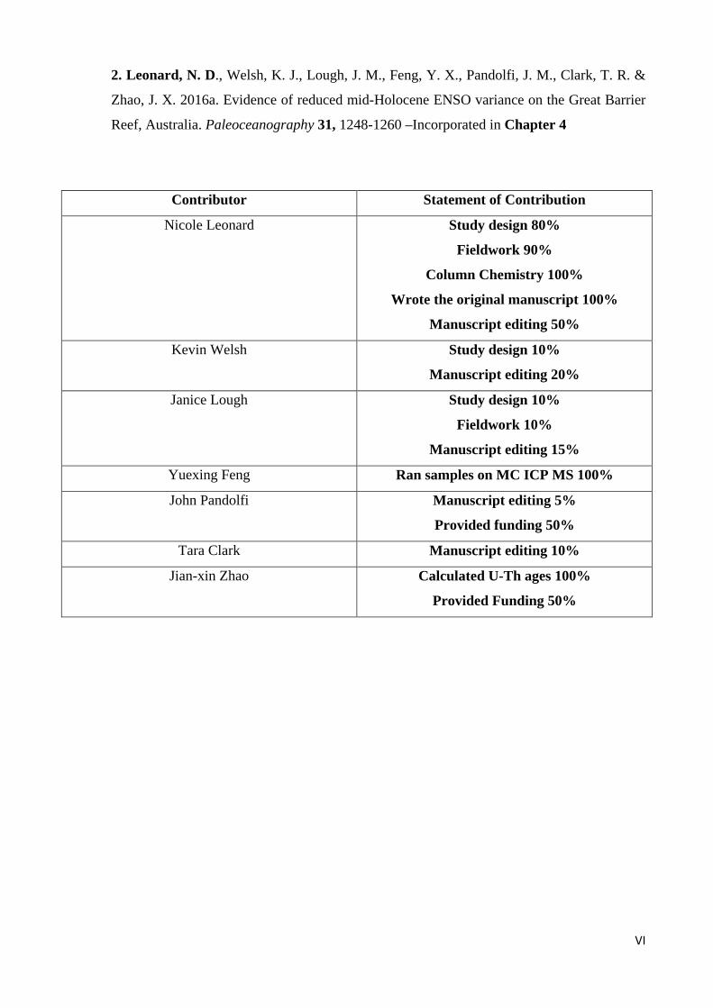
2. Leonard, N. D., Welsh, K. J., Lough, J. M., Feng, Y. X., Pandolfi, J. M., Clark, T. R. &

Zhao, J. X. 2016a. Evidence of reduced mid-Holocene ENSO variance on the Great Barrier

Reef, Australia. Paleoceanography 31, 1248-1260 –Incorporated in Chapter 4

Contributor Statement of Contribution

Nicole Leonard Study design 80%

Fieldwork 90%

Column Chemistry 100%

Wrote the original manuscript 100%


Kevin Welsh Study design 10%


Janice Lough Study design 10%

Fieldwork 10%


Yuexing Feng Ran samples on MC ICP MS 100%

John Pandolfi Manuscript editing 5%

Provided funding 50%

Tara Clark Manuscript editing 10%

Jian-xin Zhao Calculated U-Th ages 100%

Provided Funding 50%

VII

Contribution by others to the Thesis

In Leonard, N.D, Zhao, J. X., Welsh, K. J., Feng, Y. X., Smithers, S. G., Pandolfi, J. M. &

Clark, T. R. 2015. Holocene sea level instability in the southern Great Barrier Reef, Australia:

high-precision U–Th dating of fossil microatolls. Coral Reefs, 1-15 – (Chapter 2):

NDL designed the study, selected the field sites, conducted sampling and elevation surveys

prepared all samples for geochemistry, conducted column chemistry, interpreted results and

composed the initial and final versions of the manuscript. NDL, J-xZ, KJW and JMP developed the

concept of this study. SGS and TRC assisted in determining field sites and TRC assisted with

sampling and elevation surveys. Y-xF ran the analysis of samples on the Multi-collector Inductively

Coupled Mass Spectrometer (MC-ICP-MS) and J-xZ calculated U-Th ages. KJW assisted in data

interpretation, and JMP and J-xZ provided funding. All authors commented on the original and

revised versions of the manuscript prior to publication.

In Leonard, N.D., Zhao, J-x., Welsh, K.J., Feng, Y-x, Pandolfi, J.M. & Clark, T.R.,

Holocene sea level oscillations on the Great Barrier Reef and links to climate (in prep)

- (Chapter 3):

NDL designed the study, selected the field sites, conducted sampling and elevation surveys

prepared all samples for geochemistry, conducted column chemistry, interpreted results and

composed the initial and final versions of the manuscript. NDL, J-xZ, KJW and JMP developed the

concept of this study. TRC assisted with field sampling and elevation surveys. Y-xF ran the analysis

of samples on the Multi-collector Inductively Coupled Mass Spectrometer (MC-ICP-MS) and J-xZ

calculated U-Th ages. KJW assisted in data interpretation, and all authors commented on the

original and revised versions of the manuscript prior to submission.

In Leonard, N.D., Welsh, K.J., Lough J.M., Pandolfi, J.M., Clark, T.R., & Zhao, J-x.,

Evidence for reduced ENSO variance in the mid-Holocene: wavelet analysis of modern and fossil

coral luminescence indices from the Great Barrier (Paleoceanography) - (Chapter 4):

NDL designed the study, selected the corals for sampling, conducted sampling, prepared all samples

for geochemistry and conducted column chemistry for U-Th dating, conducted luminescence

analysis, statistical analysis, interpreted results and composed the initial and final versions of the

manuscript. J.M Lough provided knowledge and assistance in accessing the fossil corals. All

authors commented on the original and revised versions of the manuscript prior to submission.

VIII

In Leonard, N.D., Welsh, K.J., Nguyen, A-D., Sadler, J., Pandolfi, J.M., Clark, T.R., Zhao, J-

x. & Webb, G.E. (in prep). High resolution geochemical analysis of massive Porites sp. corals

from the Wet Tropics region, Great Barrier Reef; Rare Earth Elements and Yttrium as indicators of

terrigenous input - (Chapter 5):

NDL designed the study, selected the corals for coring, conducted sampling, prepared all samples

for geochemistry, conducted geochemical procedures, calibrated the data, conducted statistical

analysis, interpreted results and composed the initial and final versions of the manuscript. NDL, J-

xZ, KJW and JMP developed the concept of this study. TRC assisted with field sampling. A.D

Nguyen ran samples on the Quadrupole ICP-MS and assisted with geochemical procedures and data

calibration. J. Sadler assisted with sub sampling techniques for geochemistry. G.E. Webb assisted

with data interpretation. All authors commented on the original and revised versions of the

manuscript.

We are indebted to Eric Matson from the Australian Institute of Marine Science (AIMS) for

technical assistance in obtaining the fossil coral cores used in Chapter 5 and to all the staff at Hard

Rock Earth Works in Townsville for allowing access to the fossil corals and for bulldozing them

around for us. We also sincerely thank Malcolm McCullough and Juan Pablo D’Olivo from the

University of Western Australia for allowing use of their coral lab to cut the fossil coral cores and to

Gang Xi for assistance with preparation of thin sections.

Statement of parts of the thesis submitted to qualify for the award of another

degree

“None”

IX

Acknowledgements

This project was funded by the National Environment Research Programme (NERP) Tropical

Ecosystems Hub Project 1.3 to J-x. Zhao, J. Pandolfi, S. Smithers, T. Clark, Y-x. Feng and others,

Australian Research Council Linkage, Infrastructure, Equipment and Facilities (LIEF) grant

(LE0989067 for the MC-ICP-MS) to J-x. Zhao, J. Pandolfi, Y-x. Feng and others, and an Australian

Postgraduate Award to N.D.Leonard. I am also grateful for funding for international conference

attendance and travel provided by The University of Queensland School of Earth Sciences and K. J.

Welsh.

I would firstly like to thank my supervisors Dr Kevin Welsh, Prof. John Pandolfi and Prof. Jian-xin

Zhao for all the time and effort given to me throughout my PhD journey. Your individual expertise

and passion for informative science has inspired me throughout, and this thesis would not have been

possible without all of your support and advice. A very special thanks also goes out to Dr Tara

Clark for her unwavering support (and fun in the field) and Dr Yuexing Feng and Dr Ai Duc

Nguyen for their endless patience in the Radiogenic Isotope Facility. Thanks to Prof. Gregg Webb

for always having an ear for my research ideas, and to Dr G. (Dr Gilbert Price) for the motivational

pep talks. Thanks to Dr Janice Lough and Eric Matson from the Australian Institute of Marine

Science for assistance in collecting the fossil coral cores in Townsville. Much gratitude to Ashleigh

Paroz for trying to keep me on track throughout my candidature, and to the administration team in

the School of Earth Sciences that have assisted with the all the details involved in my project. To all

the staff and students, past and present, from the School of Earth Sciences who have helped keep

me somewhat sane throughout, I thank you. To the “NERP” team (Hannah Markham, Martina

Prazeres, Mauro Lapore, Beto Rodriguez-Ramirez, Juan-Pablo D’Olivo, Ian Butler and Entao Liu),

the extra supporters (James “Buddy” Sadler, Jack Coates-Marnane, and all the volunteers), and to

the boat operators involved in field work I thank you for all the hard work and fun times.

More personally I’d like to thank all my family and friends for supporting and encouraging me

throughout this journey, and for feigning interest in 6000 year old corals. To my niece Olivia (aka

bug-a-lugs) I’m sorry I didn’t manage to include mermaids in my thesis, I ran out of time! Special

thanks to Rodrigo Cardozo Ferreira for all the extra support, helping to load and unload field gear,

suffering silently with a house full of stinking coral, and making sure that I ate at least some

vegetables in the last few months of my candidature. Nuestro pequeño mundo!

X

Keywords Holocene, sea level, Great Barrier Reef, reef hiatus, microatolls, U-Th dating, rare earth element

geochemistry, coral luminescence, palaeoclimate

Australian and New Zealand Standard Research Classifications (ANZSRC)

040699 Physical Geography and Environmental Geoscience 40%

040303 Geochemistry 40%

040605 Palaeoclimatology 20%

Fields of Research (FoR) Classification

0406 Physical Geography and Environmental Geoscience 60%

0402 Geochemistry 40%

XI

Table of Contents Abstract I

Declaration by Author III

Acknowledgements IX

Table of Contents XI

List of Tables XV

List of Figures XVI

Chapter 1: Introduction

Background 1

Holocene reef growth on the Great Barrier Reef 3

Holocene sea level 5

Holocene climate 7

Objectives and Thesis outline 9

References 20

Chapter 2: Holocene sea level instability in the southern Great Barrier Reef, Australia:

high-precision U-Th dating of fossil microatolls

Abstract 30

Introduction 31

Materials and Methods

Regional Setting 33

Uranium-thorium dating 35

Results

Uranium-thorium age data 35

Age-elevation 36

Discussion and Interpretation

Mid-Holocene (6,500-4,600 yr. BP) 37

Late Holocene re-initiation (2,800 yr. BP to present) 40

Mechanisms of relative sea level oscillations

Neotectonics and hydro-isostasy 41

Climate and sea level 32

Acknowledgements 44

Funding 44

References 45

XII

Supplementary

Supplementary 1: Keppel Islands 56

Supplementary 2: Uranium-thorium methods 56

Supplementary 3: U-Th validation 58

Supplementary 4: Microatoll locations and ages 59

Supplementary References 63

Chapter 3: Holocene sea level oscillations on the Great Barrier Reef and links to climate Abstract 66

Introduction 67


Rapid sea level lowering events 70

Eustasy 71

Links to climate 72

Conclusions 73

Methods 74

Sample collection and elevation surveys 75

U-Th dating 75

Statistical analysis 76

Acknowledgements 77

References 78

Supplementary

Regional site descriptions

Far North Great Barrier Reef

Far North (12˚S, 143˚E) 83

Northern Great Barrier Reef

Alexandra Reef (16°31S, 145°28E) 84

Wet Tropics

Fitzroy Island (16˚55S, 145˚59E) 84

High Island (17˚09S, 146˚00E) 84

Central Great Barrier Reef

Stone Island (20˚02S, 148˚17E) 85 Hayman Island (20˚03S, 148˚53E) 85

Supplementary References 86

XIII

Chapter 4: Evidence for reduced ENSO variance in the mid-Holocene: wavelet analysis of

modern and fossil coral luminescence indices from the Great Barrier Reef

Abstract 100

Introduction 101

Methods

Regional Setting 104

Fossil core collection and processing 104

Data analysis 105

Results

Uranium-thorium dating 106

Wavelet analysis of modern coral luminescence 107

Wavelet analysis of fossil coral luminescence 107

Discussion 108

Wavelet transform of modern coral luminescence 108

Fossil coral analysis and ENSO 110

Conclusions 112

Acknowledgements 113

References 114

Supplementary 125

Chapter 5: High resolution geochemical analysis of massive Porites corals from the Wet

Tropics, Great Barrier Reef; rare earth elements and yttrium as indicators of

terrigenous input

Abstract 132

Introduction 133


Location and environmental setting 135

Coral core collection, treatment and sampling 136

Geochemical procedures 137

Distribution coefficients 137

Geochemical analysis 138

Results

Core chronology and growth characteristics 139


Geochemical time series 140

XIV

Variance of geochemical concentrations 140

Discussion


Geochemical time series 143

MUQ normalised REY patterns and anomalies 145

Water quality gradient; ΣREE, ΣREY and Y/Ho 146

Conclusions 147

References 149

Supplementary

Supplementary 1: Growth characteristics 162

Supplementary 2: Coral FRI 12.1 164

Supplementary 3: Geochemical statistics 166

Chapter 6: Conclusions and future directions

Conclusions 171


Coral luminescence and ENSO 173

Future research directions 174

XV

List of Tables Chapter 2: Holocene sea level instability in the southern Great Barrier Reef, Australia:


Table 1: Results of MC-ICP-MS uranium–thorium dating 50

Chapter 3: Holocene sea level oscillations on the Great Barrier Reef and links to climate Supplementary

Supp. Tbl. 1: Results of MC-ICP-MS uranium–thorium dating 88

Supp. Tbl. 2: Summary statistics for linear and Gaussian models 93



Table 1: Results of MC-ICP-MS uranium–thorium dating 119



terrigenous input

Table 1: Average rare earth element and yttrium data 153

Table 2: Summary statistics of selected geochemical data 154

Supplementary

Supp. Tbl. 1: Coral linear extension rate and tissue thickness 162

Supp. Tbl. 2: Analysis of variance (ANOVA); ΣREE, Y and Ba 166

Supp. Tbl. 3: Bonferroni adjusted t-tests; ΣREE, Y and Ba 167

XVI

List of Figures Chapter 1: Introduction

Figure 1: Map of the Great Barrier Reef, Australia 2

Figure 2: Reef core hiatus on the Great Barrier Reef, Australia 4

Figure 3: Geophysical models of relative sea level 6

Figure 4: Relative sea level data for the Australian east coast 7

Figure 5: Photographs of modern and fossil microatolls 10

Figure 6: Schematic of microatoll growth 11

Figure 7: Schematic of Morlet versus Fourier transform 15

Chapter 2: Holocene sea level instability in the southern Great Barrier Reef, Australia:


Figure 1: Map of Keppel Islands, Great Barrier Reef 52

Figure 2: Photographs of microatolls 53

Figure 3: Humpy Island age-elevation plot 54

Figure 4: Keppel Islands age-elevation plot 54

Figure 5: Inferred reef flat development North Keppel Island 55

Supplementary

Supp. Fig. 3.1: Fossil microatoll isochrons 58

Supp. Fig. 3.2: U-Th replicate measurements 58

Supp. Fig 4: Microatoll locations and ages

(a) Humpy Island 59

(b) Great Keppel Island 60

(c) North Keppel Island 61

(d) Substrate survey North Keppel Island 62

(e) Photograph of modern microatoll 62

Chapter 3: Holocene sea level oscillations on the Great Barrier Reef and links to climate Figure 1: Map of climate records and sampling sites 81

Figure 2: Microatoll age-elevation-site separated 82

Figure 3: Microatoll age-elevation-combined 83

Supplementary

Supp. Fig. 1: Photographs of fossil microatolls-Alexandra Reef 94

Supp. Fig. 2: Photographs of far north region reefs 94

XVII

Supp. Fig. 3: Photograph from Stone Island 95

Supp. Fig. 4: Linear and Gaussian models of RSL 96

Supp. Fig. 5: Selected global Holocene climate records 97



Figure 1: Map of the Palm Islands, Great Barrier Reef 120

Figure 2: Continuous wavelet transforms – modern coral 121

Figure 3: Cross wavelet transform – modern coral 122

Figure 4: Wavelet coherency – modern coral 123

Figure 5: Continuous wavelet transforms – Holocene corals 124

Supplementary

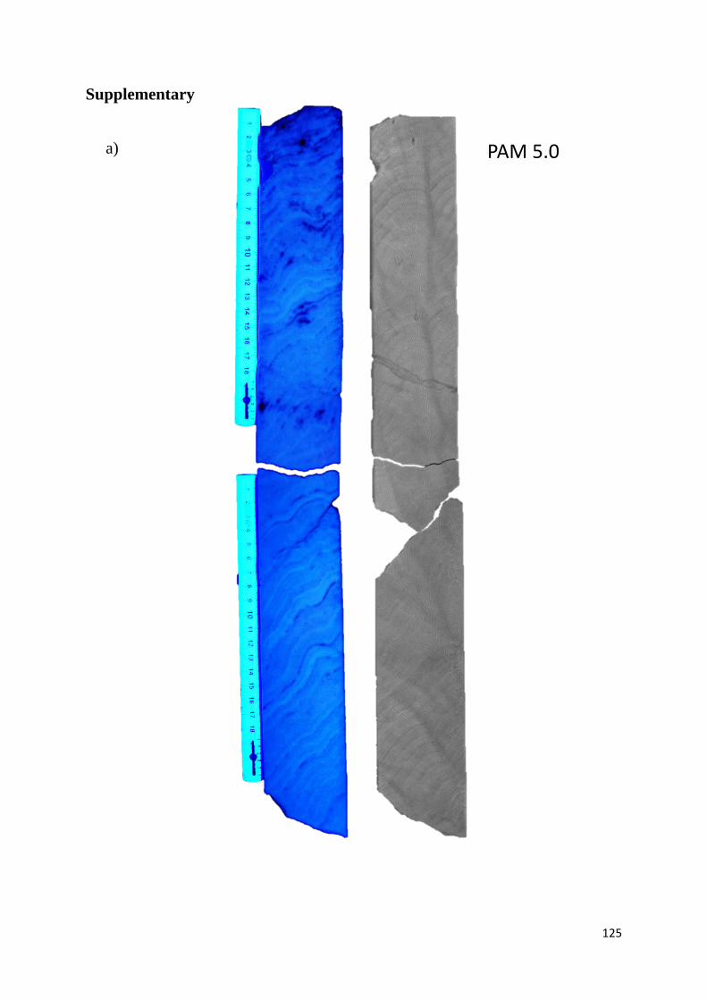
Supp. Fig. 1: Photographs and X-ray positive prints of fossil corals

(a) PAM 5.0 125

(b) PAM 2.0 126

(c) PAM 3.1 127

Supp. Fig. 2: Luminescence index data – modern and fossil corals 128

Supp. Fig. 3: Luminescence and Niño SST data 129



terrigenous input

Figure 1: Map of the Frankland Islands region and coral sites 155

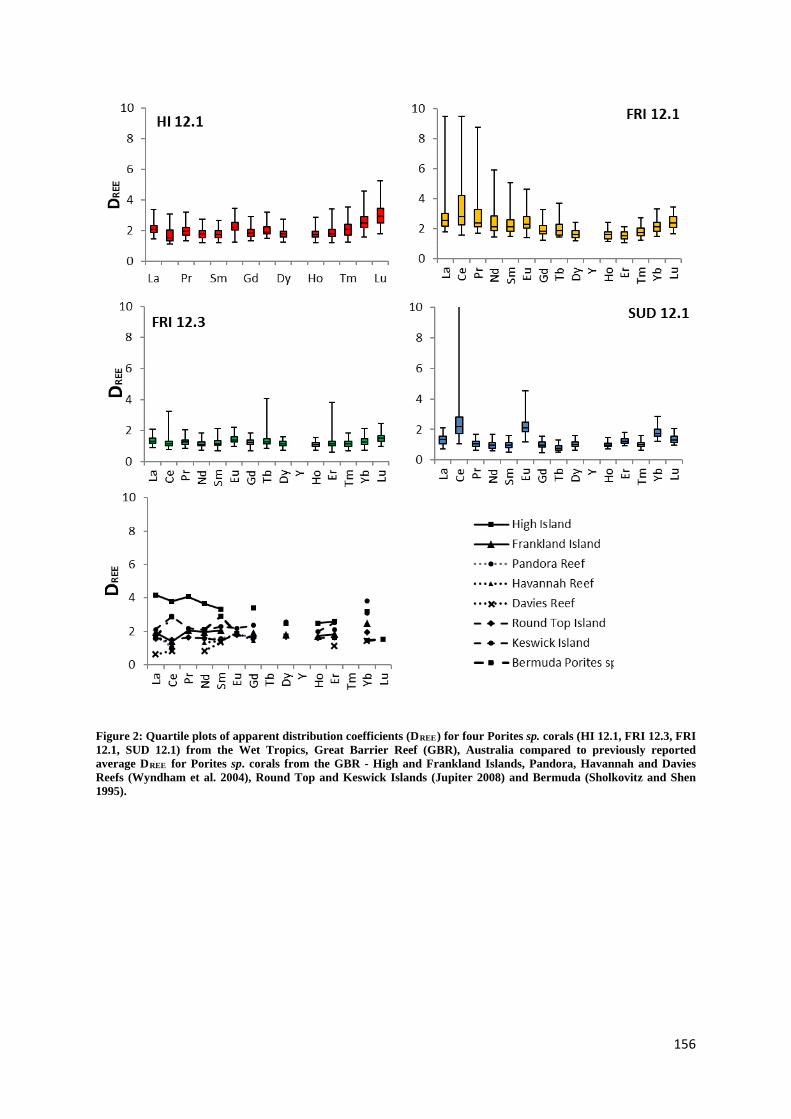
Figure 2: Quartile plots of apparent distribution coefficients 156

Figure 3: Geochemical time series; REE, Y and Ba 157

Figure 4: Scaled ΣREE time series and rainfall 158

Figure 5: MUQ normalised REY data 159

Figure 6: MUQ normalised REY; wet versus dry periods 160

Figure 7: Gridded spatial interpolation of geochemical data 161

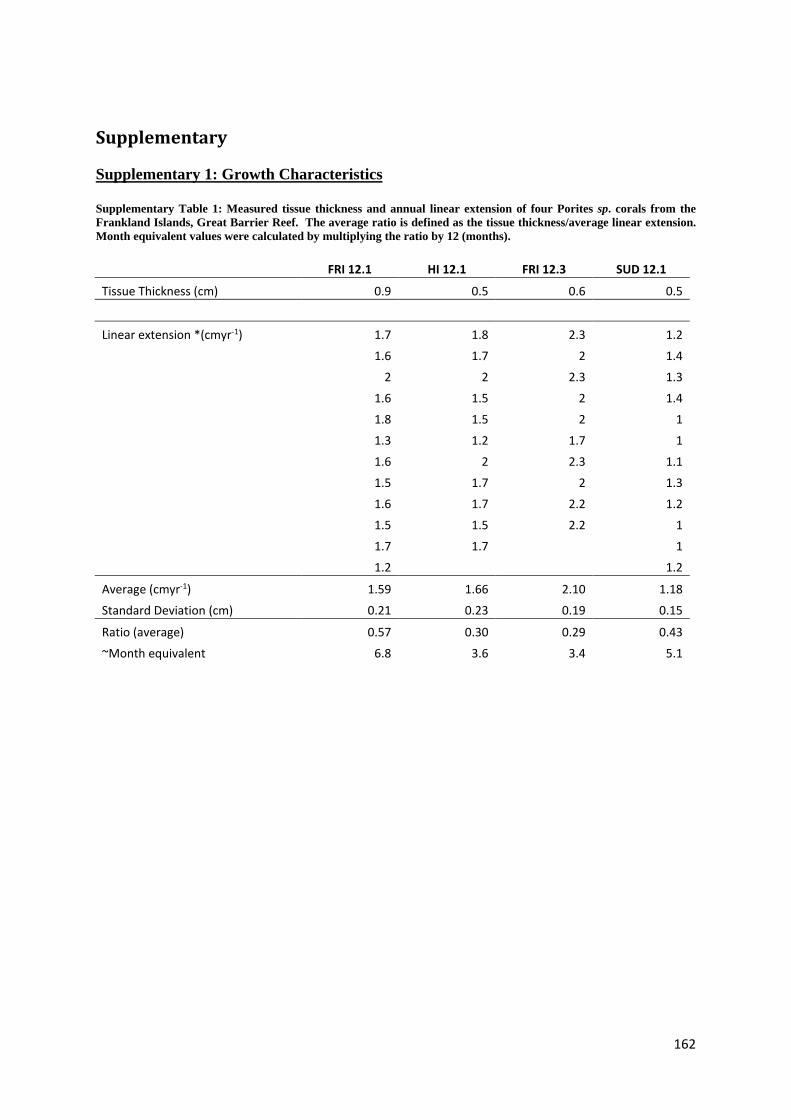
Supplementary

Supp. Fig. 1: Photographs of UV luminescent lines in Porites 163

Supp. Fig. 2: Geochemical time series data; core FRI 12.1 165

XVIII


1

Chapter 1

Introduction

Background

The recent decline of coral reefs globally is of great concern, and is often labelled as

unprecedented or more significant than in the past due to both increasing anthropogenic

impacts and climate change (Pandolfi et al., 2003, Carpenter et al., 2008, Miller et al., 2009).

The Great Barrier Reef (GBR) is no exception, with recent scrutiny by the United Nations

Educational, Scientific and Cultural Organization (UNESCO) putting the health and

management strategies of the GBR in the spotlight for all the wrong reasons (Brodie and

Waterhouse, 2012, Hughes et al., 2015).

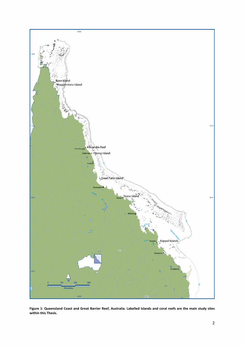
The largest contiguous reef system in the world, the GBR is a natural, social and economic

asset synonymous with Australia (Fig. 1). Spanning two thirds of the Queensland coast, it

contains over 3000 separate reefs covering an area of 345 000 km2, with ~600 of these reefs

being located in inshore environments (defined as inner-shelf, <20m bathymetry under the

influence of terrigenous deposits; Larcombe et al., 2001, Lawrence, 2010). Increased

anthropogenic pressures such as catchment clearing (Fabricius, 2005, Wooldridge, 2009, Risk

and Edinger, 2011), overfishing (Bellwood et al., 2004) and agricultural nutrient input

(Fabricius, 2005, De'ath and Fabricius, 2010, Kroon et al., 2012, Uthicke et al., 2012) are all

contributing to the decline of reefs, especially in regions within close proximity to the

coastline. Estimates suggest a ~50% reduction in coral cover since the 1960’s (Bellwood et

al., 2004, Bruno and Selig, 2007, Hughes et al., 2011) with hard coral cover declining from

27% to ~14% for the period 1985 – 2012 (De'ath et al., 2012). However, it is likely that the

true magnitude of decline may be underestimated due to the “shifting baseline” (sensu Pauly,

1995) against which modern coral assemblages are assessed (Greenstein et al., 1998, Pandolfi

et al., 2003, Knowlton and Jackson, 2008, Hughes et al., 2011, Roff et al., 2013). To enable

improved management strategies on the GBR, an evaluation of natural versus anthropogenic

drivers of change at relevant temporal resolutions is required, in conjunction with longer term

archives of coral decline (or recovery) beyond historical scientific monitoring records

(Pandolfi, 2015).

2

Figure 1: Queensland Coast and Great Barrier Reef, Australia. Labelled Islands and coral reefs are the main study sites within this Thesis.

3

Holocene reef growth on the Great Barrier Reef

Coral reef growth is constrained by a number of climatic and environmental factors such as

light, sea surface temperature (SST), turbidity, salinity and sea level (Buddemeier and

Hopley, 1988, Montaggioni, 2005, Montaggioni and Braithwaite, 2009). These factors have

also determined the geographic location of reefs throughout the Holocene, and beyond into

the deep geological past allowing for comparisons and analogues beyond the “shifting

baseline” of anthropogenic reef decline (Knowlton and Jackson, 2008, Hughes et al., 2011,

Pandolfi, 2011, Pandolfi, 2015).

The GBR as recognised today is a relatively young feature in geological terms. The oldest

date obtained from a Holocene coral is ~9500 years before present (yBP- where present is

defined as 1950; Hopley et al., 1978), with the most prolific accretion phase centred around

~7500 yBP (Smithers et al., 2006). Inshore reefs on the GBR demonstrate similarities in

patterns of reef growth history, initiating soon after inundation of the shallow Pleistocene

shelf during the post glacial marine transgression, and accreting rapidly in a either a “catch

up” or “keep up” mode of growth to ~5500 yBP (McLean et al., 1978, Stoddart et al., 1978,

Neumann and Macintyre, 1985, Kleypas and Hopley, 1992, Dullo, 2005, Montaggioni, 2005,

Hopley, 2006, Smithers et al., 2006, Perry and Smithers, 2011). Yet, after 5500 yBP the

growth history of the GBR becomes somewhat more complicated with a significant reef

“turn-off” and hiatus period of up to ~2000 years identified on many inshore reefs(Smithers

et al., 2006, Perry and Smithers, 2011).

Reef “turn-on” and “turn-off” events were initially defined by Buddemeier and Hopley

(1988) to explain periods of optimal coral growth and non-accretion/net erosion, respectively,

at significant spatial and temporal scales. On the GBR, Smithers et al. (2006) examined data

from 21 inshore and fringing reefs and discovered that Holocene reef flat progradation

reduced abruptly and significantly between 5500 and 4800 yBP. They attributed this slow

down to a scarcity of suitable substrate for further reef expansion and reduced

accommodation space due to a (smoothly) falling sea level following the mid-Holocene

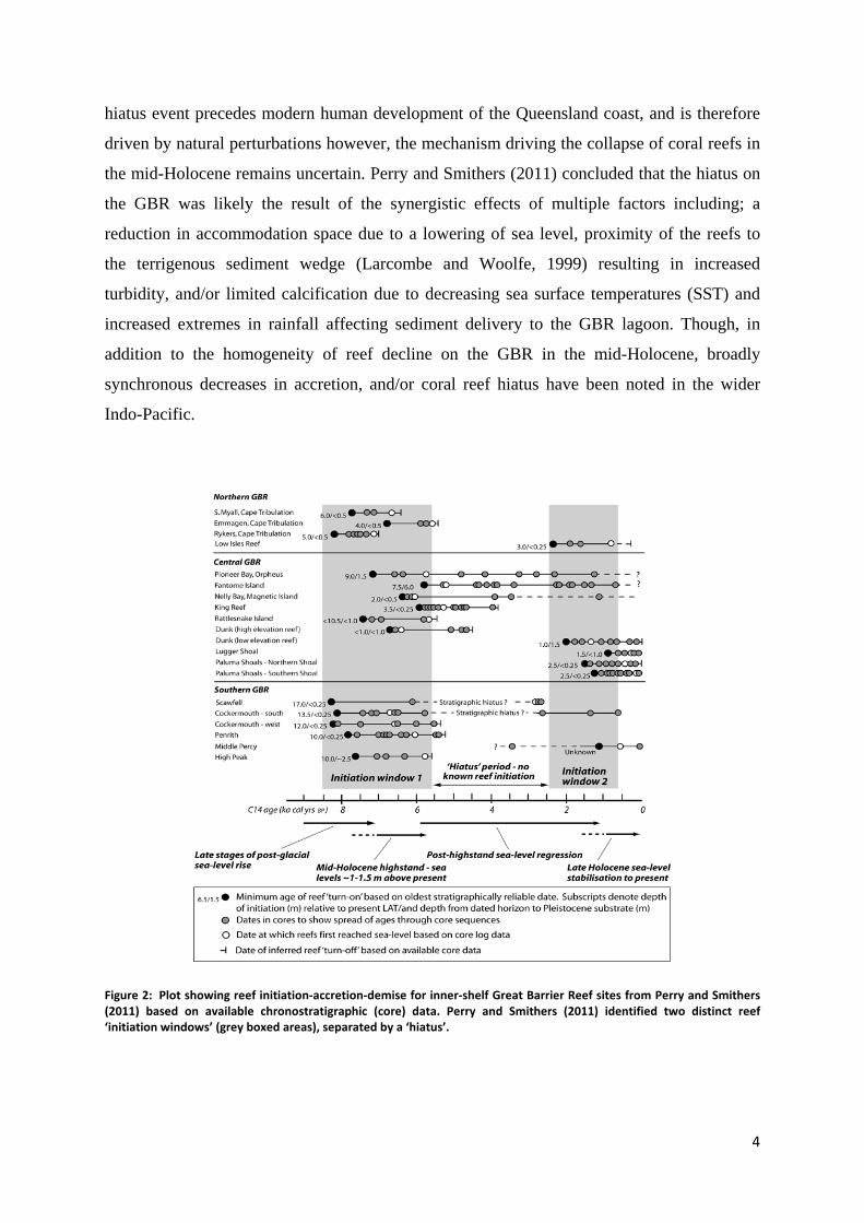
highstand. A subsequent study by Perry and Smithers (2011) examined 76 chronologically

controlled reef cores from new and previously published data from 22 reefs along the GBR,

and identified a distinct “turn off” or hiatus event occurring predominantly at inshore reefs,

and specifically in the northern and southern GBR regions, between ~5500 to 2600 yBP, with

no significant reef accretion after 4500 yBP (Fig. 2; Perry and Smithers, 2011). Clearly this

4

hiatus event precedes modern human development of the Queensland coast, and is therefore

driven by natural perturbations however, the mechanism driving the collapse of coral reefs in

the mid-Holocene remains uncertain. Perry and Smithers (2011) concluded that the hiatus on

the GBR was likely the result of the synergistic effects of multiple factors including; a

reduction in accommodation space due to a lowering of sea level, proximity of the reefs to

the terrigenous sediment wedge (Larcombe and Woolfe, 1999) resulting in increased

turbidity, and/or limited calcification due to decreasing sea surface temperatures (SST) and

increased extremes in rainfall affecting sediment delivery to the GBR lagoon. Though, in

addition to the homogeneity of reef decline on the GBR in the mid-Holocene, broadly

synchronous decreases in accretion, and/or coral reef hiatus have been noted in the wider

Indo-Pacific.

Figure 2: Plot showing reef initiation-accretion-demise for inner-shelf Great Barrier Reef sites from Perry and Smithers (2011) based on available chronostratigraphic (core) data. Perry and Smithers (2011) identified two distinct reef ‘initiation windows’ (grey boxed areas), separated by a ‘hiatus’.

5

Varying scale mechanisms have been invoked as the likely cause of these hiatus including;

eustatic sea level (ESL) oscillations (Hamanaka et al., 2012), regional relative sea level

(RSL) changes (Smithers et al., 2006, Engels et al., 2008), shifting local wave regimes

(Hongo and Kayanne, 2009), strengthening of the El Niño Southern Oscillation (ENSO;

Rooney et al., 2004, Toth et al., 2012) and an increase in intense storm activity and

subsequent sedimentation (Twiggs and Collins, 2010). Yet, the relative synchronicity of reef

decline across the Indo-Pacific in the mid-Holocene is suggestive of a possible broad scale

climatic and/or environmental shift. However high-resolution Holocene SL and climate data,

especially for the southern hemisphere and GBR, are still poorly constrained. Therefore, to

disentangle factors that have caused coral reef decline in the geological past, it is first

necessary to establish centennial to sub-centennial scale environmental and climatic

conditions that potentially led to the mid-Holocene coral hiatus.

Holocene sea level

Development of substantial three dimensional reef structures, such as those seen on the GBR,

are governed by accommodation space which is regulated by both the stage of reef

development and sea level (Veron, 1995, Dullo, 2005, Smithers et al., 2006, Perry and

Smithers, 2011, Murray-Wallace and Woodroffe, 2014). Changes to total global mean sea

level (i.e. eustatic sea level; ESL) is controlled by both changes in volume as a result of the

transfer of water storage to or from land, and the mass of the ocean due to

temperature/density changes (Lambeck et al., 2014). Following the last glacial maximum

(LGM) large scale northern hemisphere ice melt and Antarctic contributions saw ESL rise by

~ 120m between 18,000 y BP and 6000 y BP (Clark and Lingle, 1979, Fairbanks, 1989).

However water redistribution and glacio- hydroisostatic processes mean that relative sea level

histories (RSL; the level of the ocean to land) are regionally specific (Clark et al., 1978,

Milne and Mitrovica, 2008, Lambeck et al., 2014, Rovere et al., 2016). Generally, in the near

field (i.e. near to former icesheets) ice removal from continents (glacio-hydro-isostasy) is

the dominant control on the RSL signal, whereas in the far field (i.e. far from former glacial

centres) the redistribution of water (e.g. ocean syphoning) and hydroisostatic response of

continental shelves and ocean basins to increased water loads dominate (Clark et al., 1978,

Nakada and Lambeck, 1989, Lambeck and Nakada, 1990, Mitrovica and Peltier, 1991,

Pirazzoli and Pluet, 1991, Fleming et al., 1998, Lambeck, 2002, Mitrovica and Milne, 2002,

Milne and Mitrovica, 2008, Lambeck et al., 2014).

6

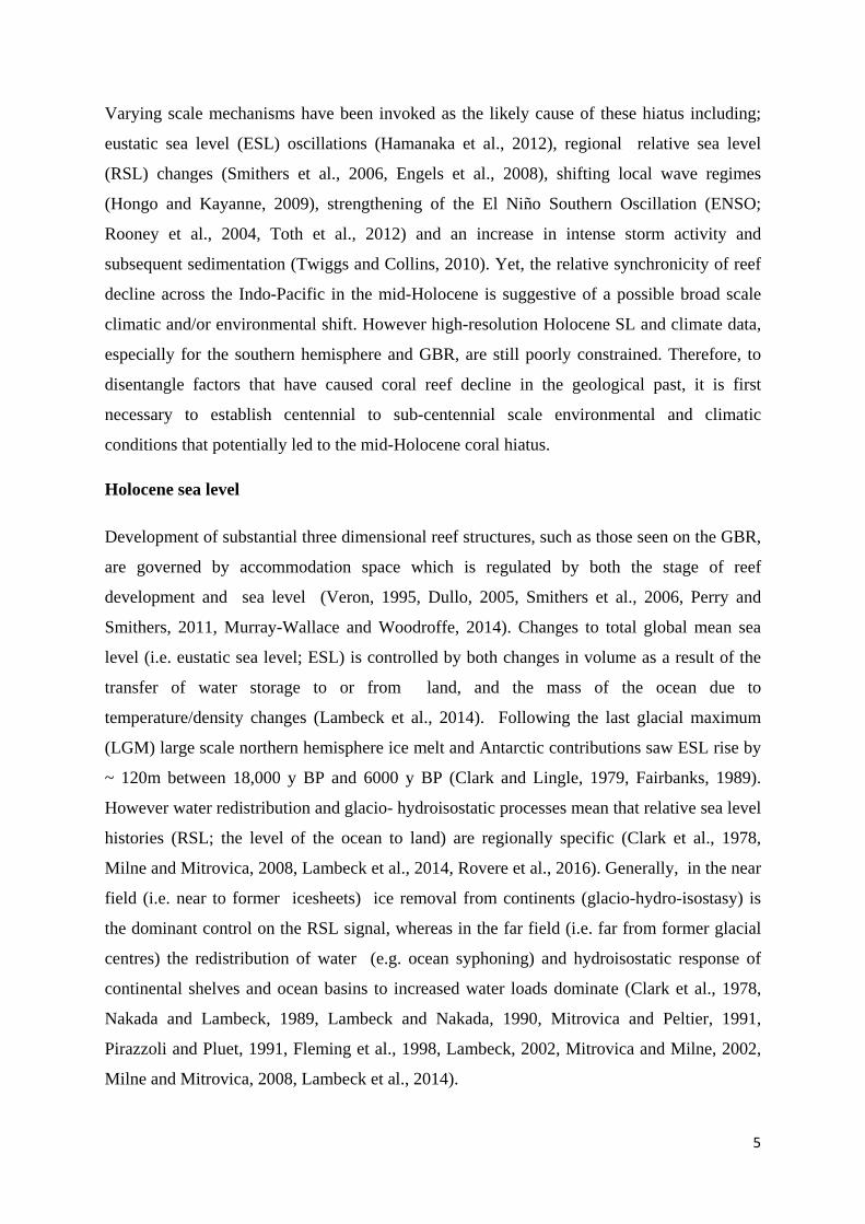
Geophysical models of regional scale RSL response to ESL change place the Australian east

coast (AEC) within a zone characterised by a mid-Holocene highstand (Fig. 3; Clark et al.,

1978) followed by a RSL fall due to water redistribution and hydroisostasy on the continental

shelf (Mitrovica and Milne, 2002). Reconstructions of RSL on the AEC using geomorphic

features (e.g. Gagan et al., 1994, Switzer et al., 2010), fixed biological indicators (e.g. Hopley

and Gill, 1972, Lewis et al., 2008), and fossil coral reefs and microatolls (Chappell, 1983b,

Chappell, 1983a, McLean and Woodroffe, 1990, Woodroffe et al., 2000) generally support a

mid-Holocene RSL highstand, although the exact magnitude and timing varies considerably

with estimates ranging between +0.7m to +3.0m between ~7500 and 5500 yBP (Chappell,

1983b, Chappell, 1983a, Fleming et al., 1998, Sloss et al., 2007, Lewis et al., 2008, Yu and

Zhao, 2010). Yet the most contentious issue is whether RSL regressed smoothly or oscillated

to present levels since the mid-Holocene highstand (Chappell, 1983a, Baker and Haworth,

2000, Horton et al., 2005, Lewis et al., 2008, Lewis et al., 2013).

Figure 3: Geophysical model of relative sea level response (sea level zones) to post glacial melt where no eustatic change in ocean volume (i.e. eustatic change) has occurred since 5000 y BP from (from Clark et al., 1978, Woodroffe and Horton, 2005).

7

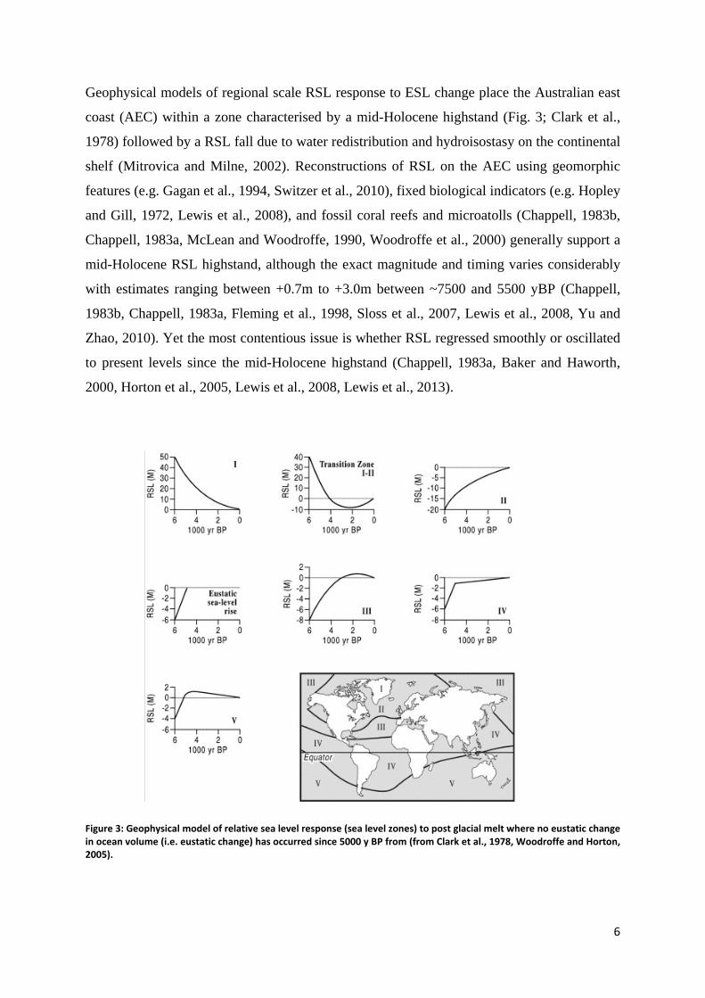
Using coral microatolls from a wide latitudinal range on the northern GBR, Chappell (1983a)

concluded that a linear, or smooth, regression was most likely. However, evidence derived

from fixed biological indicators (Baker and Haworth, 2000, Baker et al., 2005, Lewis et al.,

2008, Lewis et al., 2015) and coral microatolls (Harris et al., 2015) suggests rapid and

significant oscillations were a possibility. A comprehensive review by Lewis et al. (2008)

recalibrated previously published 14C dates of various sea level indicators from the AEC and

proposed two negative RSL oscillations centred at ~4600 and 2800 yBP, however the

persistence of the large age errors in this study limited sub-centennial interpretation (Fig. 4).

Figure 4: Recalibrated 14C sea level data from Lewis et al. (2008; and references therein) with superimposed past sea-level interpretations of Chappell et al. (1983), Larcombe et al. (1995) and Baker et al. (2005) for eastern Australia. The red bars represent growth hiatuses in oyster bed and tubeworm colonies identified by Lewis et al (2008).

Holocene climate

To enable a better understanding of coral reef response to predicted climate change and

increasing anthropogenic pressure it is also important to investigate climate conditions during

periods of reef “turn-off” throughout the Holocene. Until relatively recently the climate of

the Holocene, particularly in the Southern Hemisphere, was considered to be relatively stable

compared with prior geological epochs (Dansgaard et al., 1993, Petit et al., 1999). However,

as the number and quality of palaeoclimate data improve it is becoming evident that

8

significant and sometimes rapid climatic changes have occurred the since the end of the last

glacial maximum (Bond et al., 1997, Steig, 1999, Maslin et al., 2001, Mayewski et al., 2004,

Sang-Ik et al., 2006, Donders et al., 2008, Harrison and Bartlein, 2012). In a comprehensive

overview of global palaeoclimate records from both marine and terrestrial sources,

Mayewski et al. (2004) detected at least six rapid climate change events (over centennial

scales) during the Holocene at 9000–8000, 6000–5000, 4200–3800, 3500–2500, 1200–1000,

and 600–150 y BP. It is notable that most high resolution palaeoclimate data is currently

biased towards Northern Hemisphere records, and that complex ocean-atmospheric

teleconnections that drive global climate means that the response to these events will vary at

hemispherical to regional scales. For example, variations in the average position of the Inter-

Tropical Convergence Zone (ITCZ; e.g. Haug et al., 2001, Fleitmann et al., 2007), historical

expansion and contraction of the Indo-Pacific Warm Pool (IPWP; e.g. Abram et al., 2009, Xu

et al., 2010) and changes in the frequency and/or strength of ENSO events (e.g. Woodroffe et

al., 2003, McGregor and Gagan, 2004, Conroy et al., 2008, Cobb et al., 2013, McGregor et

al., 2013, Lough et al., 2014, Zhang et al., 2014) will differentially effect coral reefs across

the Indo-Pacific.

The El Niño Southern Oscillation (ENSO) is known to be a major driver of Australian

climate, with the position and timing of positive SST anomalies in the equatorial Pacific

controlling precipitation, storm events and general atmospheric circulation at inter-annual

time scales (Lough, 1991, Cane, 2004, Cai and Cowan, 2009, Karumuri et al., 2009,

Redondo-Rodriguez et al., 2012). The two phases of ENSO, El Niño and La Niña, produce

significant changes in effective precipitation (EP) and storm/cyclone occurrence on the AEC,

with La Niña years being wetter with higher than average SSTs and enhanced cyclone

activity, and El Niño years associated with drier and calmer conditions during the Austral

summer (Verdon et al., 2004, Meinke et al., 2005, Redondo-Rodriguez et al., 2012,

Klingaman et al., 2013, King et al., 2014). Additionally, ENSO strength and periodicity is

modulated by the Pacific Decadal Oscillation (PDO) and the Inter-decadal Pacific Oscillation

(IPO) at longer timescales (Power et al., 1999, Power et al., 2006, Verdon and Franks, 2006,

Klingaman et al., 2013, King et al., 2014, Rodriguez-Ramirez et al., 2014).

A number of reconstructions of ENSO periodicity throughout the Holocene have been

developed for the wider Pacific region from both marine [e.g. coral luminescence, Sr/Ca,

δ18O, foraminiferal Mg/Ca analyses] (Hendy et al., 2003, Woodroffe et al., 2003, McGregor

and Gagan, 2004, Cobb et al., 2013, McGregor et al., 2013, Lough et al., 2014) and terrestrial

9

proxy records (e.g. lacustrine sedimentary properties, charcoal and palynology) (Shulmeister

and Lees, 1995, Moy et al., 2002, Donders et al., 2007, Conroy et al., 2008) . It has been

suggested by several authors that ENSO amplitude was subdued during the early to mid-

Holocene [~ 9500-5000 cal. yr. BP; (Tudhope et al., 2001, McGregor and Gagan, 2004,

Brown et al., 2006, Brown et al., 2008, Wanner et al., 2008, Chiang et al., 2009, Lough et al.,

2014)] likely due to insolation characteristics (Clement et al., 2000), however spatial

inconsistencies regarding warm/cool-wet/dry phases in the Southern Hemisphere, including

the GBR region, are still unresolved (Wanner et al., 2008, Wanner et al., 2011) and may

reflect internal rather than external mechanisms [e.g. overarching phases of Pacific Decadal

Oscillations] (Debret et al., 2009, Cobb et al., 2013, Rodriguez-Ramirez et al., 2014, Emile-

geay et al., 2016).

Where palynological and sedimentary records allow for interpretation of long continuous

records of climate trends, they are limited in constraining chronologies to datable features

found within the sediment cores (Kershaw, 1983). Subsequently, although an invaluable

source of palaeoclimate data, these methods are restricted when trying to detect rapid and/or

subtle sub-decadal to centennial changes in climate (Cobb et al., 2013). High resolution

chronologically controlled coral cores address this issue, however proxy reconstructions from

Holocene coral cores on the GBR are limited to a few studies (Gagan et al., 1998, Lough et

al., 2014, Roche et al., 2014) which has resulted in a fragmented and sparse time series with

spatial inconsistencies. Consequently, more records derived from fossil corals are needed to

allow for better interpretation of high resolution environmental and climate conditions during

the Holocene, with a focus on periods for which reef hiatus have been documented.

Objectives and Thesis Outline

The primary objective of this study is to investigate climatic and environmental conditions

from the mid-Holocene to present on the Great Barrier Reef that controlled reef development

and demise. Using high precision Uranium-Thorium (U-Th) dating techniques of sub-fossil

coral microatolls (sea level) and novel treatment of coral luminescence index data from sub-

fossil Porites sp. coral cores (climate/ENSO) this study aims to describe the possible

mechanisms responsible for the previously documented reef “turn-off” event on the GBR in

the mid-Holocene.

10

Refining sub-centennial relative sea level on the Great Barrier Reef

Refining the RSL history of the GBR is paramount to understanding Holocene reef growth

histories and patterns of aggradation and progradation through time. Coral microatolls are

discoid shaped corals that have living polyps around the perimeter but for which the upper

dead flat surface has been constrained by the air-sea interface (Fig. 5a, Fig. 6 a, b) , generally

within ± 10cm of MLWS on the GBR for Porites sp. (Chappell, 1983b).

Figure 5: a) Modern microatoll emerged at lowest astronomical tide. The outer perimeter of the microatoll is living whilst the upper surface has died off as a result of exposure to the air-sea interface at ~mean low water spring tide level (MLWS). b) A field of fossil microatolls surveyed above present MLWS tide level at Alexandra Reef, Australia.

a

b

11

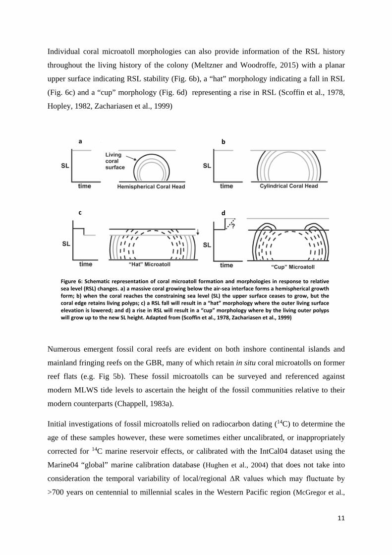
Individual coral microatoll morphologies can also provide information of the RSL history

throughout the living history of the colony (Meltzner and Woodroffe, 2015) with a planar

upper surface indicating RSL stability (Fig. 6b), a “hat” morphology indicating a fall in RSL

(Fig. 6c) and a “cup” morphology (Fig. 6d) representing a rise in RSL (Scoffin et al., 1978,

Hopley, 1982, Zachariasen et al., 1999)

Numerous emergent fossil coral reefs are evident on both inshore continental islands and

mainland fringing reefs on the GBR, many of which retain in situ coral microatolls on former

reef flats (e.g. Fig 5b). These fossil microatolls can be surveyed and referenced against

modern MLWS tide levels to ascertain the height of the fossil communities relative to their

modern counterparts (Chappell, 1983a).

Initial investigations of fossil microatolls relied on radiocarbon dating (14C) to determine the

age of these samples however, these were sometimes either uncalibrated, or inappropriately

corrected for 14C marine reservoir effects, or calibrated with the IntCal04 dataset using the

Marine04 “global” marine calibration database (Hughen et al., 2004) that does not take into

consideration the temporal variability of local/regional ΔR values which may fluctuate by

>700 years on centennial to millennial scales in the Western Pacific region (McGregor et al.,

a b

c d

Figure 6: Schematic representation of coral microatoll formation and morphologies in response to relative sea level (RSL) changes. a) a massive coral growing below the air-sea interface forms a hemispherical growth form; b) when the coral reaches the constraining sea level (SL) the upper surface ceases to grow, but the coral edge retains living polyps; c) a RSL fall will result in a “hat” morphology where the outer living surface elevation is lowered; and d) a rise in RSL will result in a “cup” morphology where by the living outer polyps will grow up to the new SL height. Adapted from (Scoffin et al., 1978, Zachariasen et al., 1999)

12

2008, Yu et al., 2010). More recently uranium-thorium (or U-series) dating has been adopted

as a method for determining coral ages, with age errors significantly reduced compared to

earlier 14C techniques (Clark et al., 2014). U-Th dating relies on the radioactive decay chain

of 238U to 206Pb via intermediate daughter products 234U and 230Th (Cheng et al., 2000,

McCulloch and Mortimer, 2008). Where uranium is soluble in seawater and taken up by

corals during skeletogenesis (between 2 - 4ppm), thorium is non-soluble and therefore

generally negligible in coral aragonite at the time of formation. By measuring the ratio

of 238U to 230Th in corals the absolute age can be calculated using the isotopic half- life

values, with corrections made for detrital contamination calculated from 232Th values

measured simultaneously (Cheng et al., 2000, Cobb et al., 2003, Shen et al., 2008).

Using microatolls dated with high-precision U-Th dating techniques this thesis aims to refine

the RSL history of the GBR throughout the Holocene. Results pertaining to this part of the

thesis are presented in Chapters 2 and 3;

Theme 1: Holocene sea level

Hypothesis 1: Temporal variations of relative sea level have controlled reef development

and demise in the Keppel Islands, GBR, throughout the Holocene.

• Local scale relative sea level, Keppel Islands – Evidence is still equivocal as to

whether RSL regressed smoothly or oscillated following the mid-Holocene highstand.

Previous sea level studies have been restricted from detecting small and possibly rapid

changes in RSL due to uncertainties and errors associated with earlier dating

techniques, and interpretation of a limited number of samples per site (generally < 10).

To evaluate relative sea level (RSL), and the pattern of sea level regression, high

precision U-Th age determinations and elevation surveys of numerous coral

microatolls were conducted on three inshore continental island fringing fossil reefs in

the Keppel Islands, southern GBR. Microatolls are precise indicators of reef phase

shifts from a vertically accreting reef matrix (“catch up”) to one that has reached RSL

and is then constrained vertically to that point (Scoffin et al., 1978, Stoddart et al.,

1978, Stoddart and Scoffin, 1979). This data provided the first evidence of a local

scale oscillatory mode of SL regression using microatolls from multiple sites within

the same region. The results of this study are presented in Chapter 2:

13

“Holocene sea level instability in the southern Great Barrier Reef, Australia: high-

precision U-Th dating of fossil microatolls”

Leonard, N.D., Zhao, J-x., Welsh, K.J., Feng, Y-x., Smithers, S.G., Pandolfi, J.M., Clark, T.R

Coral Reefs (2016)

• Regional scale sea level, Great Barrier Reef - Previous studies and syntheses of SL

on the GBR have included not only a variety of SL indicators with disparate elevation

ranges (fixed biological indicators [FBI’s], foraminiferal transfer functions, reef

cores/microatolls and geomorphological evidence), but also data combined from wide

latitudinal ranges (Hopley, 1975, Chappell, 1983a, Baker and Haworth, 2000, Baker,

2001, Sloss et al., 2007, Lewis et al., 2008, Lewis et al., 2013). This study presents 98

new microatoll U-Th age elevation points from 14 reefs presented separately across a

wide latitudinal range on the GBR (11˚S - 23˚S) based on; a) proximity to each other;

b) width of the continental shelf and; c) post-matching of SL trends. Data from this

study and from Chapter 2 are combined to further constrain Holocene RSL history on

the GBR. The results are presented in Chapter 3:

“Holocene sea level oscillations on the Great Barrier Reef and links to climate”

Leonard, N.D., Zhao, J-x, Welsh, K.J., Feng, Y-x, Clark, T.R, Pandolfi, J.M.

(In prep) – Target Journal – Nature, Nature Geoscience

Theme 2: Holocene climate and novel techniques for palaeoclimate reconstructions

High resolution mid-Holocene climate records in the southern hemisphere are currently

lacking. The second theme of this thesis is therefore concentrated on developing novel

techniques for reconstructing past climatic and environmental conditions on the GBR using

massive Porites sp. corals.

14

Annual resolution climate using coral luminescence

Fluorescent bands (or coral luminescence) revealed under ultraviolet (UV) light in annually

banded massive corals were first described by Isdale (1984), with initial investigations

suggesting that the distinct bands resulted from fluvially derived humic/fulvic acids (Boto

and Isdale, 1985, Susic et al., 1991). However, a subsequent study by Barnes and Taylor

(2005) suggests that luminescent lines are likely the result of skeletal architecture, where low

density portions of skeleton are associated with reduced salinity. This was suggested as corals

far removed from terrestrial influence were also sometimes found to exhibit luminescent lines

that could not be explained by direct humic acid contribution. Regardless, at inshore locations

luminescence bands represent river discharge events by either mechanism, and have been

used extensively to reconstruct river discharge/rainfall on the GBR (Lough, 1991, Isdale et

al., 1998, Lough et al., 2002, Fallon et al., 2003, Hendy et al., 2003, Lough, 2007, Lough,

2011b, Lough, 2011a, Lough et al., 2014, Rodriguez-Ramirez et al., 2014, Lough et al.,

2015). As precipitation on the Queensland coast is strongly modulated by wider climatic

mechanisms, luminescent lines in corals have also been used to reconstruct rainfall frequency

with links to ENSO and the Pacific Decadal Oscillation, to extend the record beyond modern

instrumentation to the past ~300 to 400 years (PDO; Isdale et al., 1998, Lough et al., 2002,

Lough, 2007, Lough, 2011b, Lough et al., 2014, Rodriguez-Ramirez et al., 2014).

Fossil coral reconstructions of ENSO variability on the GBR are currently limited (Roche et

al., 2014). Lough et al. (2014) used both modern and fossil (~6000 yBP) luminescence lines

in massive Porites to reconstruct Burdekin River discharge events, and concluded that ENSO

frequency and strength was reduced in the mid-Holocene compared to present. Roche et al.

(2014) used geochemical analysis and spectral luminescence data from a modern and fossil

microatoll from King Reef and suggested higher salinity variations, increased green/blue

spectral ratios (i.e. increased terrestrial input) and reduced Sr/Ca seasonal SST range all

represent a wetter and warmer phase on the GBR at~4600 yBP, reminiscent of modern La

Niña like conditions. Clearly more Holocene ‘windows’ derived from both coral

luminescence and geochemical proxy reconstructions are needed before a complete picture of

ENSO variability can be assessed on the GBR throughout the Holocene, however data from

elsewhere in Australia and in the wider Pacific generally supports reduced ENSO variability

and strength during the mid-Holocene (Shulmeister and Lees, 1995, Moy et al., 2002, Rodo

15

and Rodriguez-Arias, 2004, Wanner et al., 2008, Chiang et al., 2009, Carré et al., 2012, Cobb

et al., 2013, McGregor et al., 2013, Zhang et al., 2014, Emile-geay et al., 2016).

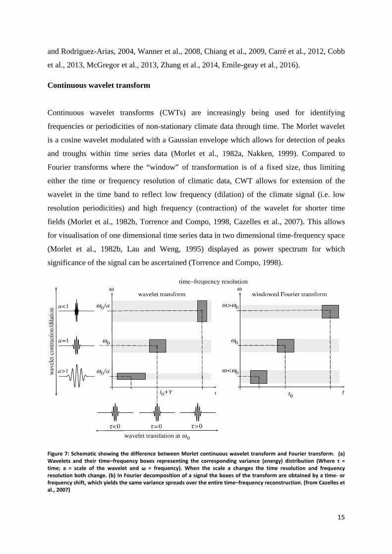
Continuous wavelet transform

Continuous wavelet transforms (CWTs) are increasingly being used for identifying

frequencies or periodicities of non-stationary climate data through time. The Morlet wavelet

is a cosine wavelet modulated with a Gaussian envelope which allows for detection of peaks

and troughs within time series data (Morlet et al., 1982a, Nakken, 1999). Compared to

Fourier transforms where the “window” of transformation is of a fixed size, thus limiting

either the time or frequency resolution of climatic data, CWT allows for extension of the

wavelet in the time band to reflect low frequency (dilation) of the climate signal (i.e. low

resolution periodicities) and high frequency (contraction) of the wavelet for shorter time

fields (Morlet et al., 1982b, Torrence and Compo, 1998, Cazelles et al., 2007). This allows

for visualisation of one dimensional time series data in two dimensional time-frequency space

(Morlet et al., 1982b, Lau and Weng, 1995) displayed as power spectrum for which

significance of the signal can be ascertained (Torrence and Compo, 1998).

Figure 7: Schematic showing the difference between Morlet continuous wavelet transform and Fourier transform. (a) Wavelets and their time–frequency boxes representing the corresponding variance (energy) distribution (Where τ = time; a = scale of the wavelet and ω = frequency). When the scale a changes the time resolution and frequency resolution both change. (b) In Fourier decomposition of a signal the boxes of the transform are obtained by a time- or frequency shift, which yields the same variance spreads over the entire time–frequency reconstruction. (from Cazelles et al., 2007)

16

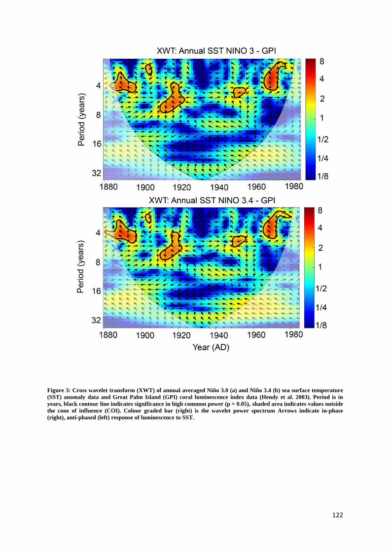
Hypothesis 2: Wavelet analysis of visually assessed ultraviolet (UV) luminescent lines in

corals enables reconstruction of past ENSO variability on the GBR.

Numerous studies are now taking advantage of continuous wavelet transforms (CWT)

of time-series environmental data (Gu and Philander, 1995, Torrence and Compo,

1998, Grinsted et al., 2004, Debret et al., 2009, Grove et al., 2013, Walther et al.,

2013, Soon et al., 2014, Lough et al., 2015) which allows for interpretation in two

dimensional time-frequency space (Torrence and Compo, 1998). This study used a

previously published record of visually assessed luminescence data from a modern

Porites sp. coral from Great Palm Island (GPI), central GBR, and Niño 3 region SST

data to assess the utility of CWTs (Morlet) in reconstructing ENSO frequency and

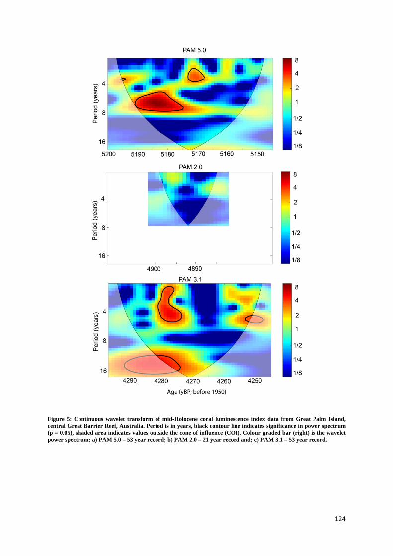
variability. The same method was then applied to three fossil Porites sp. cores from

GPI U-Th dated to ~5200, 4900 and 4300 yBP. The results of this research are

presented in Chapter 4:

“Evidence of reduced mid‐Holocene ENSO variance on the Great Barrier Reef, Australia”

Leonard, N.D., Welsh, K.J., Lough J.M., Pandolfi, J.M., Clark, T.R., Zhao, J-x.

Paleoceanography (2016)

Coral geochemistry

It is undeniable that fluvial terrigenous outputs have been altered since European settlement

on the east coast of Australia. The region has seen a fourfold increase in agriculture and

farming practise within the 38 fluvial catchments entering the GBR over the last 150 years

(Neil et al., 2002, Lawrence, 2010). Further, rapid population increases and a burgeoning

mining industry along the length of the Queensland coast has led to increased land clearing

for infrastructure (e.g. urban growth, port expansions, road development), yet limited

continuous data are available for total sediment load onto inshore reefs. Modelling studies

have reported that sediment loads to the GBR have increased 4 to 10 times since the 1850’s

(e.g. Neil et al., 2002, Kroon et al., 2012) however these models incorporate a number of

assumptions about fluvial and climatic patterns pre-disturbance for which data is limited due

17

to lack of instrumental monitoring beyond a few decades. Consequently, a number of

methods have been developed to obtain riverine sedimentary histories beyond instrumental

records either directly (e.g. sediment cores; Cavanagh et al., 1999), or by proxy (e.g. coral

geochemistry such as Barium/Calcium [Ba/Ca] and luminescence banding; Lough and

Barnes, 1997, McCulloch et al., 2003, Lewis et al., 2007).

Massive long-lived corals offer a unique opportunity to both extend the modern instrumental

record, and to reconstruct environmental conditions throughout the Holocene. When sliced

and X-radiographed, drilled cores of corals can be chronologically constrained by uranium-

thorium (U-Th) dating techniques and band counting, where one couplet of high density

(dark) and low density (light) banding in the aragonite skeleton is equal to one year of growth

(Knutson et al., 1972). Early evaluation of the geochemical composition of the aragonite of

corals recognised that trace elements and stable isotopes within the skeletal architecture

recorded numerous environmental parameters. For example, incorporation of Barium (Ba),

rare earth elements (REEs) and Yttrium (Y)have been shown to reflect the ambient chemistry

of the sea water in which the coral grew (Sholkovitz and Shen, 1995, Sinclair et al., 1998,

McCulloch et al., 2003, Dubinin, 2004). This is significant in that oceanic surface waters are

normally depleted in Ba, REEs and Y (REY), with the major source (>90%) of REYs in

coastal water is derived from suspended and dissolved riverine input (Dubinin, 2004).

Therefore, measuring the geochemically incorporated Ba and REYs in the skeletons of long-

lived massive corals can be used as a proxy to evaluate terrigenous riverine input (Shen and

Sanford, 1990).

Although numerous attempts have been made to reconcile Ba/Ca records with instrumental

data of rainfall/flood events (Alibert et al., 2003, McCulloch et al., 2003, Jupiter et al., 2008)

or known land use changes (Lewis et al., 2007), anomalous peaks and background variability

of Ba/Ca that is decoupled from flood flow data or known land use changes restricts the

interpretation of this proxy beyond the instrumental record. A number of hypothesis have

been suggested to explain possible causes of observed Ba/Ca anomalies including, tidal

mangrove sediment release of stored Ba under hyper-saline conditions during dry seasons

(Alibert et al., 2003), the significance of Ba in biological systems such as phytoplankton

blooms/scavenging processes (Lewis et al., 2007) and upwelling (McCulloch et al., 2003),

however more critical research is needed to fully understand the sources and sinks of Ba at

regional scales.

18

Low resolution (biannual) analysis of Yttrium, using solution ICP-MS, has shown promise as

a gauge of fine sediment budget to the GBR, due to its role in secondary (biological)

processes being considered insignificant (Lewis et al., 2007). Earlier studies applying LA-

ICP-MS analysis of Y also demonstrated a decreasing concentration away from sources of

sedimentary input, further suggesting that peaks may coincide with flood events (Alibert et

al., 2003), but the lower precision in this study renders interpretation equivocal. Seasonally

resolute studies of REEs, that may reflect high flow rainfall events, are to date relatively

under-examined in geochemical investigations of coral aragonite, mainly due to previously

low detection limits available and sample preparation time (Wyndham et al., 2004). As

sample protocols and detection limits of solution ICP-MS improve, investigations into utility

of REEs as a proxy of riverine terrigenous input to nearshore reefs are now more accessible.

Therefore, high-resolution analysis of REEs in chronologically-controlled annual banding of

massive corals, with particular attention to Ce and La (LREEs), are suggested to provide a

more cohesive separation of high flow riverine input onto reefs versus signals resulting from

secondary biological processes as seen in exclusive Ba/Ca analysis.

Hypothesis 3: Time series of rare earth elements and Yttrium from chronologically

controlled coral cores provides a proxy of riverine sedimentary input to coral reefs.

• Coral geochemical proxies for terrigenous input – The rare earth elements (REEs)

offer potential as a proxy for reconstructing rainfall/flood events (Wyndham et al.,

2004) and turbidity as, in coastal waters, ~90% are derived from suspended and

dissolved riverine input (Dubinin, 2004). However, few records coral REE chemistry

in massive corals from the GBR at sub-annual resolution are currently available. This

study used cores from four massive Porites sp. corals live collected from the

Frankland Islands and Sudbury Cay, a region that experiences a known water quality

gradient driven by discharge from the Russell-Mulgrave River. The geochemical

proxy data from these cores is compared with in situ data loggers (Australian Institute

of Marine Science) and river discharge, rainfall (Australian Bureau of Meteorology)

and wind data (DERM). These records have been used to determine regional

relationships between geochemical proxies in corals that can record reliable riverine

input events to inshore turbid reefs that allow for a more cohesive view of reef

sediment input histories and environmental conditions. Results of this study are

presented in Chapter 5:

19

“High resolution geochemical analysis of massive Porites sp. corals, Wet Tropics, GBR;

Rare Earth Elements and Yttrium as indicators of terrigenous input”

Leonard, N.D., Welsh, K.J., Nguyen, A.D., Sadler, J., Pandolfi, J.M., Clark, T.R., Zhao, J-x.,

Webb, G.E.

(In prep) - Target Journal – Geochimica et Cosmochimica Acta

A synthesis and general discussion of the main results of this thesis and directions for future

research is presented in Chapter 6.

20

References

Abram, N. J., Mcgregor, H. V., Gagan, M. K., Hantoro, W. S. & Suwargadi, B. W. 2009. Oscillations in the southern extent of the Indo-Pacific Warm Pool during the mid-Holocene. Quaternary Science Reviews 28, 2794-2803.

Alibert, C., Kinsley, L., Fallon, S. J., Mcculloch, M. T., Berkelmans, R. & Mcallister, F. 2003. Source of trace element variability in Great Barrier Reef corals affected by the Burdekin flood plumes. Geochimica et Cosmochimica Acta 67, 231-246.

Baker, R. 2001. Inter-tidal fixed indicators of former Holocene sea levels in Australia: a summary of sites and a review of methods and models. Quaternary International 83-85, 257-273.

Baker, R. & Haworth, R. J. 2000. Smooth or oscillating late Holocene sea-level curve? Evidence from the palaeo-zoology of fixed biological indicators in east Australia and beyond. Marine Geology 163, 367-386.

Baker, R. G. V., Haworth, R. J. & Flood, P. G. 2005. An Oscillating Holocene Sea-level? Revisiting Rottnest Island, Western Australia, and the Fairbridge Eustatic Hypothesis. Journal of Coastal Research Special Issue, 3-14.

Barnes, D. J. & Taylor, R. B. 2005. On the nature and causes of luminescent lines and bands in coral skeletons: II. Contribution of skeletal crystals. Journal of experimental marine biology and ecology 322, 135-142.

Bellwood, D. R., Hughes, T. P., Folke, C. & Nyström, M. 2004. Confronting the coral reef crisis. Nature 429, 827-833.

Bond, G., Bonani, G., Showers, W., Cheseby, M., Lotti, R., Almasi, P., Demenocal, P., Priore, P., Cullen, H. & Hajdas, I. 1997. A Pervasive Millennial-Scale Cycle in North Atlantic Holocene and Glacial Climates. Science 278, 1257-1266.

Boto, K. & Isdale, P. 1985. Fluorescent bands in massive corals result from terrestrial fulvic acid inputs to nearshore zone. Nature 315, 396-397.

Brodie, J. & Waterhouse, J. 2012. A critical review of environmental management of the 'not so Great' Barrier Reef. Estuarine, Coastal and Shelf Science 104-105, 1.

Brown, J., Collins, M. & Tudhope, A. 2006. Coupled model simulations of mid-Holocene ENSO and comparisons with coral oxygen isotope records. Advances in Geosciences 6, 29-33.

Brown, J., Collins, M., Tudhope, A. W. & Toniazzo, T. 2008. Modelling mid-Holocene tropical climate and ENSO variability: towards constraining predictions of future change with palaeo-data. Climate Dynamics 30, 19-36.

Bruno, J. F. & Selig, E. R. 2007. Regional Decline of Coral Cover in the Indo-Pacific: Timing, Extent, and Subregional Comparisons. PloS one 2, e711.

Buddemeier, R. W. & Hopley, D. Turn-ons and Turn-offs; Causes and mechanisms of the initiation and termination of coral reef growth. In: Proceedings of the 6th International Coral Reef Symposium, 1988 Australia. 253 - 261.

Cai, W. & Cowan, T. 2009. La Niña Modoki impacts Australia autumn rainfall variability. Geophysical Research Letters 36, L12805.

Cane, M. A. 2004. The evolution of El Niño, past and future. Earth and Planetary Science Letters 230, 227-240.

Carpenter, K. E., Abrar, M., Aeby, G., Aronson, R. B., Banks, S., Bruckner, A., Chiriboga, A., Cortés, J., Delbeek, J. C., Devantier, L., Edgar, G. J., Edwards, A. J., Fenner, D., Guzmán, H. M., Hoeksema, B. W., Hodgson, G., Johan, O., Licuanan, W. Y., Livingstone, S. R., Lovell, E. R., Moore, J. A., Obura, D. O., Ochavillo, D., Polidoro, B. A., Precht, W. F., Quibilan, M. C., Reboton, C., Richards, Z. T., Rogers, A. D., Sanciangco, J., Sheppard, A., Sheppard, C., Smith, J., Stuart, S., Turak, E., Veron, J. E. N., Wallace, C., Weil, E. & Wood, E. 2008. One-Third of Reef-Building Corals Face Elevated Extinction Risk from Climate Change and Local Impacts. Science 321, 560-563.

Carré, M., Azzoug, M., Bentaleb, I., Chase, B. M., Fontugne, M., Jackson, D., Ledru, M.-P., Maldonado, A., Sachs, J. P. & Schauer, A. J. 2012. Mid-Holocene mean climate in the south eastern Pacific and its influence on South America. Quaternary International 253, 55-66.

21

Cavanagh, J. E., Burns, K. A., Brunskill, G. J. & Coventry, R. J. 1999. Organochlorine Pesticide Residues in Soils and Sediments of the Herbert and Burdekin River Regions, North Queensland – Implications for Contamination of the Great Barrier Reef. Marine Pollution Bulletin 39, 367-375.

Cazelles, B., Chavez, M., Magny, G. C. D., Guégan, J.-F. & Hales, S. 2007. Time-dependent spectral analysis of epidemiological time-series with wavelets. Journal of The Royal Society Interface 4, 625-636.

Chappell, J. 1983a. Evidence for smoothly falling sea-level relative to North Queensland, Australia, during the past 6,000 yr. Nature 302, 406-408.

Chappell, J. 1983b. Holocene palaeo-environmental changes, Central to North Great Barrier Reef inner zone. BMR Journal of Australian Geology and Geophysics 8, 223-235.

Cheng, H., Edwards, R. L., Hoff, J., Gallup, C. D., Richards, D. A. & Asmerom, Y. 2000. The half-lives of uranium-234 and thorium-230. Chemical Geology 169, 17-33.

Chiang, J. C. H., Fang, Y. & Chang, P. 2009. Pacific Climate Change and ENSO Activity in the Mid-Holocene. Journal of Climate 22, 923-939.

Clark, J. A., Farrell, W. E. & Peltier, W. R. 1978. Global changes in postglacial sea level: A numerical calculation. Quaternary Research 9, 265-287.

Clark, J. A. & Lingle, C. S. 1979. Predicted relative sea-level changes (18,000 years B.P. to present) caused by late-glacial retreat of the Antarctic Ice Sheet. Quaternary Research 11, 279-298.

Clark, T. R., Roff, G., Zhao, J.-X., Feng, Y.-X., Done, T. J. & Pandolfi, J. M. 2014. Testing the precision and accuracy of the U–Th chronometer for dating coral mortality events in the last 100 years. Quaternary Geochronology 23, 35-45.

Clement, A. C., Seager, R. & Cane, M. A. 2000. Suppression of El Niño during the Mid-Holocene by changes in the Earth's orbit. Paleoceanography 15, 731-737.

Cobb, K. M., Charles, C. D., Cheng, H., Kastner, M. & Edwards, R. L. 2003. U/Th-dating living and young fossil corals from the central tropical Pacific. Earth and Planetary Science Letters 210, 91-103.

Cobb, K. M., Westphal, N., Sayani, H. R., Watson, J. T., Di Lorenzo, E., Cheng, H., Edwards, R. L. & Charles, C. D. 2013. Highly variable El Niño-Southern Oscillation throughout the Holocene. Science (New York, N.Y.) 339, 67.

Conroy, J. L., Overpeck, J. T., Cole, J. E., Shanahan, T. M. & Steinitz-Kannan, M. 2008. Holocene changes in eastern tropical Pacific climate inferred from a Galápagos lake sediment record. Quaternary Science Reviews 27, 1166-1180.

Dansgaard, W., Johnsen, S., Clausen, H., Dahl-Jensen, D., Gundestrup, N., Hammer, C., Hvidberg, C., Steffensen, J., Sveinbjörnsdottir, A. & Jouzel, J. 1993. Evidence for general instability of past climate from a 250-kyr ice-core record. Nature 364, 218-220.

De'ath, G. & Fabricius, K. 2010. Water quality as a regional driver of coral biodiversity and macroalgae on the Great Barrier Reef. Ecological Applications 20, 840-850.

De'ath, G., Fabricius, K. E., Sweatman, H. & Puotinen, M. 2012. The 27-year decline of coral cover on the Great Barrier Reef and its causes. Proceedings of the National Academy of Sciences of the United States of America 109, 17995-17999.

Debret, M., Sebag, D., Crosta, X., Massei, N., Petit, J. R., Chapron, E. & Bout-Roumazeilles, V. 2009. Evidence from wavelet analysis for a mid-Holocene transition in global climate forcing. Quaternary Science Reviews 28, 2675-2688.

Donders, T. H., Haberle, S. G., Hope, G., Wagner, F. & Visscher, H. 2007. Pollen evidence for the transition of the Eastern Australian climate system from the post-glacial to the present-day ENSO mode. Quaternary Science Reviews 26, 1621-1637.

Donders, T. H., Wagner-Cremer, F. & Visscher, H. 2008. Integration of proxy data and model scenarios for the mid-Holocene onset of modern ENSO variability. Quaternary Science Reviews 27, 571-579.

Dubinin, A. V. 2004. Geochemistry of Rare Earth Elements in the Ocean. Lithology and Mineral Resources 39, 289-289.

Dullo, W.-C. 2005. Coral growth and reef growth: a brief review. Facies 51, 33-48. Emile-Geay, J., Cobb, K. M., Carré, M., Braconnot, P., Leloup, J., Zhou, Y., Harrison, S. P., Corrège,

T., Mcgregor, H. V., Collins, M., Driscoll, R., Elliot, M., Schneider, B. & Tudhope, A. 2016.

22

Links between tropical Pacific seasonal, interannual and orbital variability during the Holocene. Nature Geoscience 9, 168.

Engels, M. S., Fletcher, C. H., Field, M., Conger, C. L. & Bochicchio, C. 2008. Demise of reef-flat carbonate accumulation with late Holocene sea-level fall: evidence from Molokai, Hawaii. Coral Reefs 27, 991-996.

Fabricius, K. E. 2005. Effects of terrestrial runoff on the ecology of corals and coral reefs: review and synthesis. Marine Pollution Bulletin 50, 125-146.

Fairbanks, R. G. 1989. A 17,000-year glacio-eustatic sea level record: influence of glacial melting rates on the Younger Dryas event and deep-ocean circulation. Nature 342, 637.

Fallon, S., Wyndham, T., Hendy, E., Lough, J. & Barnes, D. 2003. Coral record of increased sediment flux to the inner Great Barrier Reef since European settlement. Nature 421, 727-730.

Fleitmann, D., Burns, S. J., Mangini, A., Mudelsee, M., Kramers, J., Villa, I., Neff, U., Al-Subbary, A. A., Buettner, A., Hippler, D. & Matter, A. 2007. Holocene ITCZ and Indian monsoon dynamics recorded in stalagmites from Oman and Yemen (Socotra). Quaternary Science Reviews 26, 170-188.

Fleming, K., Johnston, P., Zwartz, D., Yokoyama, Y., Lambeck, K. & Chappell, J. 1998. Refining the eustatic sea-level curve since the Last Glacial Maximum using far- and intermediate-field sites. Earth and Planetary Science Letters 163, 327-342.

Gagan, M. K., Ayliffe, L. K., Hopley, D., Cali, J. A., Mortimer, G. E., Chappell, J., Mcculloch, M. T. & Head, M. J. 1998. Temperature and Surface-Ocean Water Balance of the Mid-Holocene Tropical Western Pacific. Science 279, 1014-1018.

Gagan, M. K., Johnson, D. P. & Crowley, G. M. 1994. Sea level control of stacked late Quaternary coastal sequences, central Great Barrier Reef. Sedimentology 41, 329-351.

Greenstein, B., Curran, H. & Pandolfi, J. 1998. Shifting ecological baselines and the demise of Acropora cervicornis in the western North Atlantic and Caribbean Province: a Pleistocene perspective. Coral Reefs 17, 249-261.

Grinsted, A., Moore, J. C. & Jevrejeva, S. 2004. Application of the cross wavelet transform and wavelet coherence to geophysical time series. Nonlinear Processes in Geophysics 11, 561-566.

Grove, C. A., Zinke, J., Peeters, F., Park, W., Scheufen, T., Kasper, S., Randriamanantsoa, B., Mcculloch, M. T. & Brummer, G. J. A. 2013. Madagascar corals reveal a multidecadal signature of rainfall and river runoff since 1708. Climate of the Past 9, 641-656.

Gu, D. & Philander, S. G. H. 1995. Secular Changes of Annual and Interannual Variability in the Tropics during the Past Century. Journal of Climate 8, 864-876.

Hamanaka, N., Kan, H., Yokoyama, Y., Okamoto, T., Nakashima, Y. & Kawana, T. 2012. Disturbances with hiatuses in high-latitude coral reef growth during the Holocene: Correlation with millennial-scale global climate change. Global and Planetary Change 80-81, 21-35.

Harris, D. L., Webster, J. M., Vila-Concejo, A., Hua, Q., Yokoyama, Y. & Reimer, P. J. 2015. Late Holocene sea-level fall and turn-off of reef flat carbonate production: Rethinking bucket fill and coral reef growth models. Geology 43, 175-178.

Harrison, S. P. & Bartlein, P. 2012. Chapter 14 - Records from the Past, Lessons for the Future: What the Palaeorecord Implies about Mechanisms of Global Change. In: Ann, H.-S. & Kendal, M. (eds.) The Future of the World's Climate (Second Edition). Boston: Elsevier.

Haug, G. H., Hughen, K. A., Sigman, D. M., Peterson, L. C. & Röhl, U. 2001. Southward migration of the intertropical convergence zone through the Holocene. Science (New York, N.Y.) 293, 1304-1308.

Hendy, E. J., Gagan, M. K. & Lough, J. 2003. Chronological control of coral records using luminescent lines and evidence for non-stationary ENSO teleconnections in northeast Australia. The Holocene 13, 187-199.

Hongo, C. & Kayanne, H. 2009. Holocene coral reef development under windward and leeward locations at Ishigaki Island, Ryukyu Islands, Japan. Sedimentary Geology 214, 62-73.

Hopley, D. 1975. Contrasting evidence for Holocene sea levels with special reference to the Bowen-Whitsunday area of Queensland. Douglas, I., I-Iobbs, JE and Pigram, JJ (eds.) Geographical Essays in Honour ofGilbert J Butland, Dept. Geogr., Univ. New England, Armidale 5, 1-84.

23

Hopley, D. 1982. The geomorphology of the Great Barrier Reef: quaternary development of coral reefs, New York, Wiley.

Hopley, D. 2006. Fringing and Nearshore Coral Reefs of the Great Barrier Reef: Episodic Holocene Development and Future Prospects. Journal of Coastal Research 22, 175-187.

Hopley, D. & Gill, E. 1972. Holocene sea levels in eastern Australia — A discussion. Marine Geology 12, 223-233.

Hopley, D., Mclean, R. F., Marshall, J. F. & Smith, A. S. 1978. Holocene-Pleistocene boundary in a fringing reef:Hayman Island, North Queensland. Search 9, 323-325.

Horton, B. P., Gibbard, P. L., Mine, G. M., Morley, R. J., Purintavaragul, C. & Stargardt, J. M. 2005. Holocene sea levels and palaeoenvironments, Malay-Thai Peninsula, southeast Asia. The Holocene 15, 1199-1213.

Hughen, K., Lehman, S., Southon, J., Overpeck, J., Marchal, O., Herring, C. & Turnbull, J. 2004. 14C Activity and Global Carbon Cycle Changes over the past 50,000 Years. Science 303, 202-207.

Hughes, T. P., Bellwood, D. R., Baird, A. H., Brodie, J., Bruno, J. F. & Pandolfi, J. M. 2011. Shifting base-lines, declining coral cover, and the erosion of reef resilience: comment on Sweatman et al. (2011). Coral Reefs 30, 653-660.

Hughes, T. P., Day, J. C. & Brodie, J. 2015. Securing the future of the Great Barrier Reef. Nature Climate Change 5, 508-511.

Isdale, P. 1984. Fluorescent bands in massive corals record centuries of coastal rainfall. Nature 310, 578-579.

Isdale, P. J., Stewart, B. J., Tickle, K. S. & Lough, J. M. 1998. Palaeohydrological variation in a tropical river catchment: a reconstruction using fluorescent bands in corals of the Great Barrier Reef, Australia. The Holocene 8, 1-8.

Jupiter, S., Roff, G., Marion, G., Henderson, M., Schrameyer, V., Mcculloch, M. & Hoegh-Guldberg, O. 2008. Linkages between coral assemblages and coral proxies of terrestrial exposure along a cross-shelf gradient on the southern Great Barrier Reef. Coral Reefs 27, 887-903.

Karumuri, A., Tam, C. Y. & Lee, W. J. 2009. ENSO Modoki impact on the Southern Hemisphere storm track activity during extended austral winter. Geophysical Research Letters 36, L12705.

Kershaw, A. P. 1983. A Holocene Pollen Diagram from Lynch's Crater, North-Eastern Queensland, Australia. New Phytologist 94, 669-682.

King, A. D., Klingaman, N. P., Alexander, L. V., Donat, M. G., Jourdain, N. C. & Maher, P. 2014. Extreme Rainfall Variability in Australia: Patterns, Drivers, and Predictability. Journal of Climate 27, 6035.

Kleypas, J. A. & Hopley, D. Reef Development Across a Broad Continental Shelf, Southern Great Barrier Reef, Australia. In: Richmond, R. H., ed. Seventh International Coral Reef Symposium, 1992 Guam. University of Guam Press, 1129-1141.

Klingaman, N. P., Woolnough, S. J. & Syktus, J. 2013. On the drivers of inter‐annual and decadal rainfall variability in Queensland, Australia. International Journal of Climatology 33, 2413-2430.

Knowlton, N. & Jackson, J. B. C. 2008. Shifting Baselines, Local Impacts, and Global Change on Coral Reefs. PLoS Biol 6, e54.

Knutson, D. W., Buddemeier, R. W. & Smith, S. V. 1972. Coral chronometers: Seasonal growth bands in reef corals. Science 177, 270-272.

Kroon, F. J., Kuhnert, P. M., Henderson, B. L., Wilkinson, S. N., Kinsey-Henderson, A., Abbott, B., Brodie, J. E. & Turner, R. D. R. 2012. River loads of suspended solids, nitrogen, phosphorus and herbicides delivered to the Great Barrier Reef lagoon. Marine Pollution Bulletin 65, 167-181.

Lambeck, K. 2002. Sea level change from mid Holocene to recent time: an Australian example with global implications. Geodynamics Series 29, 33-50.

Lambeck, K. & Nakada, M. 1990. Late Pleistocene and Holocene sea-level change along the Australian coast. Palaeogeography, Palaeoclimatology, Palaeoecology (Global and Planetary Change Section) 89, 143-176.

24

Lambeck, K., Rouby, H., Purcell, A., Sun, Y. & Sambridge, M. 2014. Sea level and global ice volumes from the Last Glacial Maximum to the Holocene. Proceedings of the National Academy of Sciences 111, 15296-15303.

Larcombe, P., Costen, A. & Woolfe, K. J. 2001. The hydrodynamic and sedimentary setting of nearshore coral reefs, central Great Barrier Reef shelf, Australia: Paluma Shoals, a case study. Sedimentology 48, 811-835.

Larcombe, P. & Woolfe, K. J. 1999. Terrigenous sediments as influences upon Holocene nearshore coral reefs, central Great Barrier Reef, Australia. Australian Journal of Earth Sciences 46, 141-154.

Lau, K.-M. & Weng, H. 1995. Climate Signal Detection Using Wavelet Transform: How to Make a Time Series Sing. Bulletin of the American Meteorological Society 76, 2391-2402.

Lawrence, K. 2010. Social and economic profile of the Great Barrier Reef catchment 2009. Townsville, Qld.: Great Barrier Reef Marine Park Authority.

Lewis, S. E., Shields, G. A., Kamber, B. S. & Lough, J. M. 2007. A multi-trace element coral record of land-use changes in the Burdekin River catchment, NE Australia. Palaeogeography, Palaeoclimatology, Palaeoecology 246, 471-487.

Lewis, S. E., Sloss, C. R., Murray-Wallace, C. V., Woodroffe, C. D. & Smithers, S. G. 2013. Post-glacial sea-level changes around the Australian margin: a review. Quaternary Science Reviews 74, 115-138.

Lewis, S. E., Wu, R. a. J., Webster, J. M. & Shields, G. A. 2008. Mid-late Holocene sea-level variability in eastern Australia. Terra Nova 20, 74-81.

Lewis, S. E., Wüst, R. a. J., Webster, J. M., Collins, J., Wright, S. A. & Jacobsen, G. 2015. Rapid relative sea-level fall along north-eastern Australia between 1200 and 800 cal. yr BP: An appraisal of the oyster evidence. Marine Geology 370, 20-30.

Lough, J., Barnes, D. & Mcallister, F. 2002. Luminescent lines in corals from the Great Barrier Reef provide spatial and temporal records of reefs affected by land runoff. Coral Reefs 21, 333-343.

Lough, J. M. 1991. Rainfall variations in Queensland, Australia: 1891–1986. International Journal of Climatology 11, 745-768.

Lough, J. M. 2007. Tropical river flow and rainfall reconstructions from coral luminescence: Great Barrier Reef, Australia. Paleoceanography 22.

Lough, J. M. 2011a. Great Barrier Reef coral luminescence reveals rainfall variability over northeastern Australia since the 17th century. Paleoceanography 26.

Lough, J. M. 2011b. Measured coral luminescence as a freshwater proxy: comparison with visual indices and a potential age artefact. Coral Reefs 30, 169-182.

Lough, J. M. & Barnes, D. J. 1997. Several centuries of variation in skeletal extension, density and calcification in massive Porites colonies from the Great Barrier Reef: A proxy for seawater temperature and a background of variability against which to identify unnatural change. Journal of experimental marine biology and ecology 211, 29-67.

Lough, J. M., Lewis, S. E. & Cantin, N. E. 2015. Freshwater impacts in the central Great Barrier Reef: 1648–2011. Coral Reefs 34, 739-751.

Lough, J. M., Llewellyn, L. E., Lewis, S. E., Turney, C. S. M., Palmer, J. G., Cook, C. G. & Hogg, A. G. 2014. Evidence for suppressed mid‐Holocene northeastern Australian monsoon variability from coral luminescence. Paleoceanography 29, 581-594.

Maslin, M., Stickley, C. & Ettwein, V. 2001. Holocene Climate Variability. In: Editors-in-Chief: john, H. S., Karl, K. T. & Steve, A. T. (eds.) Encyclopedia of Ocean Sciences (Second Edition). Oxford: Academic Press.

Mayewski, P. A., Holmgren, K., Lee-Thorp, J., Rosqvist, G., Rack, F., Staubwasser, M., Schneider, R. R., Steig, E. J., Rohling, E. E., Curt Stager, J., Karlén, W., Maasch, K. A., David Meeker, L., Meyerson, E. A., Gasse, F. & Van Kreveld, S. 2004. Holocene climate variability. Quaternary Research 62, 243-255.

Mcculloch, M., Fallon, S., Wyndham, T., Hendy, E., Lough, J. & Barnes, D. 2003. Coral record of increased sediment flux to the inner Great Barrier Reef since European settlement. Nature 421, 727-730.

25

Mcculloch, M. T. & Mortimer, G. E. 2008. Applications of the 238U–230Th decay series to dating of fossil and modern corals using MC-ICPMS. Australian Journal of Earth Sciences 55, 955-965.

Mcgregor, H. V., Fischer, M. J., Gagan, M. K., Fink, D., Phipps, S. J., Wong, H. & Woodroffe, C. D. 2013. A weak El Niño/Southern Oscillation with delayed seasonal growth around 4,300 years ago. Nature Geoscience 6, 949-953.

Mcgregor, H. V. & Gagan, M. K. 2004. Western Pacific coral δ18O records of anomalous Holocene variability in the El-Nino-Southern Oscillation. Geophysical Research Letters 31, 1-4.

Mcgregor, H. V., Gagan, M. K., Mcculloch, M. T., Hodge, E. & Mortimer, G. 2008. Mid-Holocene variability in the marine 14C reservoir age for northern coastal Papua New Guinea. Quaternary Geochronology 3, 213-225.

Mclean, R. & Woodroffe, C. 1990. Microatolls and recent sea level change on coral atolls. Nature 344, 531-534.

Mclean, R. F., Stoddart, D. R., Hopley, D. & Polach, H. 1978. Sea Level Change in the Holocene on the Northern Great Barrier Reef. Philosophical Transactions of the Royal Society of London. Series A, Mathematical and Physical Sciences 291, 167-186.

Meinke, H., Devoil, P., Hammer, G. L., Power, S., Allan, R., Stone, R. C., Folland, C. & Potgieter, A. 2005. Rainfall Variability at Decadal and Longer Time Scales: Signal or Noise? Journal of Climate 18, 89-96.

Meltzner, A. J. & Woodroffe, C. D. 2015. Coral microatolls. Handbook of Sea-Level Research. John Wiley & Sons, Ltd.

Miller, J., Muller, E., Rogers, C., Waara, R., Atkinson, A., Whelan, K., Patterson, M. & Witcher, B. 2009. Coral disease following massive bleaching in 2005 causes 60% decline in coral cover on reefs in the US Virgin Islands. Coral Reefs 28, 925-937.

Milne, G. A. & Mitrovica, J. X. 2008. Searching for eustasy in deglacial sea-level histories. Quaternary Science Reviews 27, 2292-2302.

Mitrovica, J. X. & Milne, G. A. 2002. On the origin of late Holocene sea-level highstands within equatorial ocean basins. Quaternary Science Reviews 21, 2179-2190.

Mitrovica, J. X. & Peltier, W. R. 1991. On Postglacial Geoid Subsidence Over the Equatorial Oceans. Journal of Geophysical Research 96, 20053-20071.

Montaggioni, L. F. 2005. History of Indo-Pacific coral reef systems since the last glaciation: Development patterns and controlling factors. Earth Science Reviews 71, 1-75.

Montaggioni, L. F. & Braithwaite, C. J. R. 2009. Chapter One Introduction: Quaternary Reefs in Time and Space. In: Montaggioni, L. F. & Braithwaite, C. J. R. (eds.) Developments in Marine Geology. Elsevier.

Morlet, J., Arens, G., Fourgeau, E. & Giard, D. 1982a. Wave Propagation and Sampling Theory-Part 1: Complex Signal and Scattering in Multilayered Media. Geophysics 47, 203-221.

Morlet, J., Arens, G., Fourgeau, E. & Giard, D. 1982b. Wave propagation and sampling Theory - Part II: Sampling theory and complex waves. Geophysics 47, 222-236.

Moy, C. M., Anderson, D. M., Seltzer, G. O. & Rodbell, D. T. 2002. Variability of El Niño/Southern Oscillation activity at millennial timescales during the Holocene epoch. Nature 420, 162-165.

Murray-Wallace, C. V. & Woodroffe, C. D. 2014. Quaternary sea-level changes: a global perspective. Cambridge;New York;: Cambridge University Press.

Nakada, M. & Lambeck, K. 1989. Late Pleistocene and Holocene sea-level change in the Australian region and mantle rheology. Geophysical Journal International 96, 497-517.

Nakken, M. 1999. Wavelet analysis of rainfall–runoff variability isolating climatic from anthropogenic patterns. Environmental Modelling and Software 14, 283-295.

Neil, D. T., Orpin, A. R., Ridd, P. V. & Yu, B. 2002. Sediment yield and impacts from river catchments to the Great Barrier Reef lagoon.

Neumann, A. C. & Macintyre, I. G. Reef response to sea level rise: keep-up, catch up or give-up. In: Proc. 5th Int Coral Reef Congr, 1985 Tahiti. 105-110.

Pandolfi, J. M. 2011. The Paleoecology of Coral Reefs. Dordrecht: Springer Netherlands. Pandolfi, J. M. 2015. Incorporating Uncertainty in Predicting the Future Response of Coral Reefs to

Climate Change. Annual Review of Ecology, Evolution, and Systematics 46, 281-303.

26

Pandolfi, J. M., Bradbury, R. H., Sala, E., Hughes, T. P., Bjorndal, K. A., Cooke, R. G., Mcardle, D., Mcclenachan, L., Newman, M. J. H., Paredes, G., Warner, R. R. & Jackson, J. B. C. 2003. Global Trajectories of the Long-Term Decline of Coral Reef Ecosystems. Science 301, 955-958.

Pauly, D. 1995. Anecdotes and the shifting baseline syndrome of fisheries. Trends in Ecology and Evolution 10, 430.

Perry, C. & Smithers, S. 2011. Cycles of coral reef 'turn-on', rapid growth and 'turn-off' over the past 8500 years: a context for understanding modern ecological states and trajectories. Global Change Biology 17, 76-86.

Petit, J.-R., Jouzel, J., Raynaud, D., Barkov, N. I., Barnola, J.-M., Basile, I., Bender, M., Chappellaz, J., Davis, M. & Delaygue, G. 1999. Climate and atmospheric history of the past 420,000 years from the Vostok ice core, Antarctica. Nature 399, 429-436.

Pirazzoli, P. A. & Pluet, J. 1991. World atlas of Holocene sea-level changes, Amsterdam ; New York, Elsevier.

Power, S., Casey, T., Folland, C., Colman, A. & Mehta, V. 1999. Inter-decadal modulation of the impact of ENSO on Australia. Climate Dynamics 15, 319-324.

Power, S., Haylock, M., Colman, R. & Wang, X. 2006. The predictability of interdecadal changes in ENSO activity and ENSO teleconnections. Journal of Climate 19, 4755-4771.

Redondo-Rodriguez, A., Weeks, S. J., Berkelmans, R., Hoegh-Guldberg, O. & Lough, J. M. 2012. Climate variability of the Great Barrier Reef in relation to the tropical Pacific and El Niño-Southern Oscillation. Marine and Freshwater Research 63, 34.

Risk, M. J. & Edinger, E. 2011. Encyclopedia of modern coral reefs: structure, form and process. In: Hopley, D. (ed.). Dordrecht: Springer.

Roche, R. C., Perry, C. T., Smithers, S. G., Leng, M. J., Grove, C. A., Sloane, H. J. & Unsworth, C. E. 2014. Mid-Holocene sea surface conditions and riverine influence on the inshore Great Barrier Reef. The Holocene 24, 885-897.

Rodo, X. & Rodriguez-Arias, M.-A. 2004. El Nino-Southern Oscillation: Absent in the Early Holocene? Journal of Climate 17, 423-426.

Rodriguez-Ramirez, A., Grove, C. A., Zinke, J., Pandolfi, J. M. & Zhao, J.-X. 2014. Coral Luminescence Identifies the Pacific Decadal Oscillation as a Primary Driver of River Runoff Variability Impacting the Southern Great Barrier Reef. PloS one 9, e84305.

Roff, G., Clark, T. R., Reymond, C. E., Zhao, J.-X., Feng, Y., Mccook, L. J., Done, T. J. & Pandolfi, J. M. 2013. Palaeoecological evidence of a historical collapse of corals at Pelorus Island, inshore Great Barrier Reef, following European settlement. Proceedings. Biological sciences / The Royal Society 280.

Rooney, J., Fletcher, C., Grossman, E., Engels, M. & Field, M. 2004. El Nino Influence on Holocene Reef Accretion in Hawai'i1. Pacific Science 58, 305.

Rovere, A., Stocchi, P. & Vacchi, M. 2016. Eustatic and Relative Sea Level Changes. Current Climate Change Reports, 1-11.

Sang-Ik, S., Prashant, D. S., Robert, S. W., Robert, J. O. & Joseph, J. B. 2006. Understanding the Mid-Holocene Climate. Journal of Climate 19, 2801.

Scoffin, T. P., Stoddart, D. R. & Rosen, B. R. 1978. The Nature and Significance of Microatolls. Philosophical Transactions of the Royal Society of London. Series B, Biological Sciences 284, 99-122.

Shen, C.-C., Fan, T.-Y., Meltzner, A. J., Taylor, F. W., Quinn, T. M., Chiang, H.-W., Kilbourne, K. H., Li, K.-S., Sieh, K., Natawidjaja, D., Cheng, H., Wang, X., Edwards, R. L., Lam, D. D. & Hsieh, Y.-T. 2008. Variation of initial 230Th/ 232Th and limits of high precision U–Th dating of shallow-water corals. Geochimica et Cosmochimica Acta 72, 4201-4223.

Shen, G. T. & Sanford, C. L. 1990. Trace element indicators of climate variability in reef-building corals. Global ecological consequences of the 1982-83 El Nino-Southern Oscillation, 255-283.

Sholkovitz, E. & Shen, G. T. 1995. The incorporation of rare earth elements in modern coral. Geochimica et Cosmochimica Acta 59, 2749-2756.

Shulmeister, J. & Lees, B. G. 1995. Pollen evidence from tropical Australia for the onset of an ENSO-dominated climate at c. 4000 BP. The Holocene 5, 10-18.

27

Sinclair, D. J., Kinsley, L. P. J. & Mcculloch, M. T. 1998. High resolution analysis of trace elements in corals by laser ablation ICP-MS. Geochimica et Cosmochimica Acta 62, 1889-1901.

Sloss, C. R., Murray-Wallace, C. V. & Jones, B. G. 2007. Holocene sea-level change on the southeast coast of Australia: a review. The Holocene 17, 999.

Smithers, S. G., Hopley, D. & Parnell, K. E. 2006. Fringing and Nearshore Coral Reefs of the Great Barrier Reef: Episodic Holocene Development and Future Prospects. Journal of Coastal Research, 175-187.

Soon, W., Velasco Herrera, V. M., Selvaraj, K., Traversi, R., Usoskin, I., Chen, C.-T. A., Lou, J.-Y., Kao, S.-J., Carter, R. M., Pipin, V., Severi, M. & Becagli, S. 2014. A review of Holocene solar-linked climatic variation on centennial to millennial timescales: Physical processes, interpretative frameworks and a new multiple cross-wavelet transform algorithm. Earth-Science Reviews 134, 1-15.

Steig, E. J. 1999. Mid-Holocene Climate Change. Science 286, 1485-1487. Stoddart, D. R., Mclean, R. F., Scoffin, T. P., Thom, B. G. & Hopley, D. 1978. Evolution of Reefs

and Islands, Northern Great Barrier Reef: Synthesis and Interpretation. Philosophical Transactions of the Royal Society of London. Series B, Biological Sciences 284, 149-159.

Stoddart, D. R. & Scoffin, T. P. 1979. Microatolls: Review of Form, Origin and Terminology. Atoll Research Bulletin No. 224, 1-17.

Susic, M., Boto, K. & Isdale, P. 1991. Fluorescent humic acid bands in coral skeletons originate from terrestrial runoff. Marine Chemistry 33, 91-104.

Switzer, A., Sloss, C. R., Jones, B. G. & Bristow, C. 2010. Geomorphic evidence for mid-late Holocene higher sea level from southeastern Australia. Quaternary International 221, 13-22.

Torrence, C. & Compo, G. P. 1998. A practical guide to wavelet analysis. Bulletin of the American Meteorological Society 79, 61-78.

Toth, L. T., Macintyre, I. G., Aronson, R. B., Vollmer, S. V., Hobbs, J. W., Urrego, D. H., Cheng, H., Enochs, I. C., Combosch, D. J. & Van Woesik, R. 2012. ENSO drove 2500-year collapse of eastern Pacific coral reefs. Science (New York, N.Y.) 337, 81.

Tudhope, A. W., Chilcott, C. P., Mcculloch, M. T., Cook, E. R., Chappell, J., Ellam, R. M., Lea, D. W., Lough, J. M. & Shimmield, G. B. 2001. Variability in the El Niño-Southern Oscillation through a glacial-interglacial cycle. Science (New York, N.Y.) 291, 1511-1517.

Twiggs, E. J. & Collins, L. B. 2010. Development and demise of a fringing coral reef during Holocene environmental change, eastern Ningaloo Reef, Western Australia. Marine Geology 275, 20-36.

Uthicke, S., Patel, F. & Ditchburn, R. 2012. Elevated land runoff after European settlement perturbs persistent foraminiferal assemblages on the Great Barrier Reef. Ecology 93, 111-121.

Verdon, D. C. & Franks, S. W. 2006. Long-term behaviour of ENSO: Interactions with the PDO over the past 400 years inferred from paleoclimate records. Geophysical Research Letters 33, L06712.

Verdon, D. C., Wyatt, A. M., Kiem, A. S. & Franks, S. W. 2004. Multidecadal variability of rainfall and streamflow: Eastern Australia. Water Resources Research 40, W10201.

Veron, J. E. N. 1995. Corals in space and time: the biogeography and evolution of the Scleractinia, Ithaca, Comstock/Cornell.

Walther, B. D., Kingsford, M. J. & Mcculloch, M. T. 2013. Environmental Records from Great Barrier Reef Corals: Inshore versus Offshore Drivers. PloS one 8, e77091.

Wanner, H., Beer, J., Bütikofer, J., Crowley, T. J., Cubasch, U., Flückiger, J., Goosse, H., Grosjean, M., Joos, F., Kaplan, J. O., Küttel, M., Müller, S. A., Prentice, I. C., Solomina, O., Stocker, T. F., Tarasov, P., Wagner, M. & Widmann, M. 2008. Mid- to Late Holocene climate change: an overview. Quaternary Science Reviews 27, 1791-1828.

Wanner, H., Solomina, O., Grosjean, M., Ritz, S. P. & Jetel, M. 2011. Structure and origin of Holocene cold events. Quaternary Science Reviews 30, 3109-3123.

Woodroffe, C. D., Beech, M. R. & Gagan, M. K. 2003. Mid-late Holocene El Niño variability in the equatorial Pacific from coral microatolls. Geophysical Research Letters 30, 1358.

Woodroffe, C. D. & Horton, B. P. 2005. Holocene sea-level changes in the Indo-Pacific. Journal of Asian Earth Sciences 25, 29-43.

28

Woodroffe, C. D., Kennedy, D. M., Hopley, D., Rasmussen, C. E. & Smithers, S. G. 2000. Holocene reef growth in Torres Strait. Marine Geology 170, 331-346.

Wooldridge, S. A. 2009. Water quality and coral bleaching thresholds: Formalising the linkage for the inshore reefs of the Great Barrier Reef, Australia. Marine Pollution Bulletin 58, 745-751.

Wyndham, T., Mcculloch, M., Fallon, S. & Alibert, C. 2004. High-resolution coral records of rare earth elements in coastal seawater: biogeochemical cycling and a new environmental proxy. Geochimica et Cosmochimica Acta 68, 2067-2080.

Xu, J., Kuhnt, W., Holbourn, A., Regenberg, M. & Andersen, N. 2010. Indo-Pacific Warm Pool variability during the Holocene and Last Glacial Maximum. Paleoceanography 25, PA4230.

Yu, K.-F. & Zhao, J.-X. 2010. U-series dates of Great Barrier Reef corals suggest at least +0.7m sea level ~7000 years ago. The Holocene 20, 161-168.

Yu, K., Hua, Q., Zhao, J.-X., Hodge, E., Fink, D. & Barbetti, M. 2010. Holocene marine 14C reservoir age variability: Evidence from 230Th-dated corals in the South China Sea. Paleoceanography 25.

Zachariasen, J., Sieh, K., Taylor, F. W., Edwards, L. & Hantoro, W. S. 1999. Submergence and uplift associated with the giant 1833 Sumatran subduction earthquake: Evidence from coral microatolls. Journal of Geophysical Research: Solid Earth 104, 895-919.

Zhang, Z., Leduc, G. & Sachs, J. P. 2014. El Nino evolution during the Holocene revealed by a biomarker rain gauge in the Galapagos Islands. Earth and Planetary Science Letters 404, 420.

29

Chapter 2

Holocene sea level instability in the southern Great Barrier Reef, Australia: high-precision U-Th dating of

fossil microatolls

Nicole D Leonard1,2, Zhao, J-x.1,2, Welsh, K.J.1, Feng, Y-x1,2, Smithers, S.G.3, Pandolfi, J.M.4, Clark, T.R1,2.

1. School of Earth Sciences, The University of Queensland; St Lucia, Queensland, 4072.

2. Radiogenic Isotope Facility, The University of Queensland; St Lucia, Queensland, 4072.

3. School of Earth and Environmental Sciences, James Cook University; Townsville, Queensland, 4811.

4. Australian Research Council Centre of Excellence for Coral Reef Studies, Centre for Marine Science, School of Biological Sciences, The University of Queensland, Brisbane,

Queensland 4072.

Published: Coral Reefs (2016) 35: 625

Keywords: Sea level; Holocene; Great Barrier Reef; microatoll; uranium-thorium; reef hiatus

30

Abstract

Three emergent sub-fossil reef flats from the inshore Keppel Islands, Great Barrier Reef

(GBR), Australia, were used to reconstruct relative sea level (RSL). Forty-two high-precision

uranium-thorium (U-Th) dates obtained from coral microatolls and non-microatoll colonies

(2σ age errors from ± 8 to 37 years) in conjunction with elevation surveys provide evidence

in support of a non-linear RSL regression throughout the Holocene. Results show that RSL

was as least 0.75 m above present from ~6,500 – 5,500 years before present (yr. BP; before

1950). Following this highstand, two sites indicate a coeval lowering of RSL of at least 0.4 m

from 5,500 – 5,300 yr. BP which was maintained for ~200 years. After the lowstand, RSL

returns to higher levels before a 2,000 year hiatus in reef flat corals after 4,600 yr. BP at all

three sites. A second possible RSL lowering event of ~0.3 m from ~2,800 –1,600 yr. BP is

then detected before RSL stabilises ~0.2 m above present levels by 900 yr. BP. Whilst the

mechanism of the RSL instability is still uncertain, the alignment with previously reported

RSL oscillations, rapid global climate changes and mid-Holocene reef “turn-off” on the GBR

are discussed.

31

Introduction

It is indisputable that coral reefs are under increasing pressure from anthropogenic influence

globally (Pandolfi et al., 2003, Veron et al., 2009, Muthukrishnan and Fong, 2014).

Nevertheless, natural processes have equally affected reef development throughout geological

history, and worldwide coral reefs have suffered significant disturbances and hiatuses prior to

anthropogenic influence (Buddemeier and Hopley, 1988, Hughes and Connell, 1999,

Smithers et al., 2006, Perry and Smithers, 2011, Hamanaka et al., 2012, Toth et al., 2012).

Determining the driving mechanisms of previous reef disturbance events is not only vital to

interpreting Holocene reef histories, but allows for improved understanding of the future

trajectory of reefs under changing climatic and environmental conditions.

Eustatic sea level (ESL) transgressive/regressive cycles are one of the primary controls of

coral reef expansion/contraction throughout the Quaternary (Kennedy and Woodroffe, 2002,

Hopley et al., 2007). Where ESL is dominated by changes in ice sheet volume and global

steric variations, relative sea level (RSL) at any given coastline is governed by ESL

contributions, as well as regional glacio-hydro-isostatic and tectonic effects (Lambeck and

Nakada, 1990, Lambeck, 1993, Lambeck et al., 2014), water redistribution (Mitrovica and

Milne, 2002) and climate (Hamanaka et al., 2012). At near-field sites (i.e. close to former

icesheets and melt water) glacio-isostatic influence on RSL is dominant, however at far-field

locations (distant from major ice accumulations) RSL at centennial to millennial timescales is

mainly controlled by hydro-isostasy, equatorial ocean syphoning and steric effects which can

produce significant spatial and temporal variability over just a few hundred kilometres

(Lambeck and Nakada, 1990, Mitrovica and Milne, 2002).

Geophysical modelling of the regional response to glacio-hydro-isostatic processes has

resulted in the identification of distinct zones of globally predicted RSL throughout the

Holocene (Clark et al., 1978, Pirazzoli and Pluet, 1991). The islands and reefs of the inshore

Great Barrier Reef (GBR), proximal to the mainland Queensland coast are characterised by a

rapidly rising RSL from the early to mid-Holocene, culminating in a RSL highstand of +1 to

+3 m by ~5,000 years before present after which significant meltwater contribution from the

large northern hemisphere icesheets ceased (Clark et al., 1978, Nakada and Lambeck, 1989).

Evidence of this highstand along the Australian east coast (AEC) between 7,000 – 5,000

years before present (yr. B.P; where present is 1950) is widespread and widely accepted

(McLean et al., 1978, Hopley, 1980, Chappell et al., 1982, Chappell, 1983, Woodroffe et al.,

32

2000, Lewis et al., 2008, Yu and Zhao, 2010b, Leonard et al., 2013), although the magnitude

and precise timing of the highstand is yet to be unequivocally refined (see Lewis et al., 2008

and , Lewis et al., 2013 for comprehensive reviews of Australian sea level throughout the

Holocene).

Inshore reef development on the GBR reflects the rapid early to mid-Holocene RSL rise with

coral initiation following inundation of the shallow Pleistocene shelf from ~8,500 yr. BP,

followed by rapid reef accretion in either “catch up” or “keep up” modes of growth until

~5,500 yr. BP (Neumann and Macintyre, 1985, Kleypas and Hopley, 1992, Smithers et al.,

2006, Perry and Smithers, 2011, Camoin and Webster, 2015). After ~5,500cal yr. BP

however, both RSL and reef growth histories become increasingly ambiguous. Whether RSL

regressed smoothly (Chappell, 1983) or oscillated/stepped down (Baker and Haworth, 2000,

Baker, 2001, Lewis et al., 2008) on the AEC following the mid-Holocene highstand has been

a contentious issue for over four decades. Indeed, different statistical treatments of the same

sea level (SL) data suggests either regression mode to be equally likely (Woodroffe, 2009).

At the same time, stratigraphic hiatuses in coral reef cores and a lack of reef initiation in the

northern and southern inshore GBR have been documented from 5,500 – 2,800 yr. BP,

suggestive of significant environmental change at this time, yet this hiatus is not detected in

the central GBR (Perry and Smithers, 2011). Perry and Smithers (2011) proposed that a

reduction in vertical accommodation space due to a slowly falling RSL in synergy with

changes to environmental conditions at inshore locations (e.g. temperature, rainfall and shore

progradation) limited significant reef aggradation/progradation in the mid-Holocene.

However, such a synchronous and broad-scale response is suggestive of either a more abrupt

change in RSL than currently proposed for the GBR (Chappell, 1983), or that rapid and

wide scale climatic and environmental change was the primary driver of reef “turn-off”

(Buddemeier and Hopley, 1988).

Whilst rapid changes or oscillations of RSL during the Holocene have been proposed for the

AEC, they are most often dismissed as artefacts of the proxies used and uncertainties of age-

error calculations (Perry and Smithers, 2011). In order to obtain a temporally continuous

record it is often necessary to incorporate dissimilar SL indicators, or SL indicators from

large latitudinal ranges, into a single interpretation potentially obscuring subtle variations

(Chappell, 1983, Sloss et al., 2007, Lewis et al., 2008, Lewis et al., 2013). Additionally,

directly comparing or combining data from separate studies is problematic as: a) the

reference datum and the absolute elevation of the indicators being used may differ; b)

33

inconsistent methods between studies are used to establish elevation and age; c) large age

errors may be associated with dating techniques [e.g. for 14C dating, substantial age errors up

to ± 500 years may be introduced if temporal changes in atmospheric production rates as well

as global and regional marine 14C reservoir effects are taken into consideration (McGregor et

al., 2008, Yu et al., 2010, Hua et al., 2015)]; and d) the environmental context of the

indicators is critically important but is often difficult to interpret and commonly not reported.

The primary objective of this study was to determine whether low magnitude RSL instability

could be detected using highly precise U-Th dating techniques of coral microatolls from

multiple sites in a tectonically stable far-field region. In addition, we also obtained samples of

non-microatolls to relate dated microatolls to reef flat development at their time of growth.

This sampling regime allowed for both intra- and inter-site comparisons of equivalent data,

thereby increasing the confidence in the absolute RSL signal versus single reef

geomorphological effects. This study is the first comprehensive evaluation of Holocene RSL

and reef flat history in the Keppel Islands, a region for which data has been notably absent

(Hopley et al., 2007, Lewis et al., 2013).


Regional Setting

The Keppel Islands are a group of continental islands located on the inner shelf of the

southern GBR, Queensland, Australia (23˚10’S, 150˚59’E; Fig. 1). The islands are located in

a macro tidal setting with a maximum tidal range of ~5 m. The region experiences a

seasonally dry tropical climate in which most (on average 60%) of the rainfall typically

occurs in the short wet season between December and March (B.O.M., 2011). Inter-annual

variability is also high, with long dry periods often followed by episodic high flow rainfall

events associated with tropical cyclones or monsoonal lows (Douglas et al., 2006, Brooke et

al., 2008) which are modulated by complex interactions of the El Niño Southern Oscillation

(ENSO) and Pacific Decadal Oscillation (Rodriguez-Ramirez et al., 2014). Due to frequent

disturbance events (e.g. cyclones flood plumes) the modern Keppel Islands reefs are

dominated by fast growing arborescent Acropora sp. (see Supp. 1). Although it has been

suggested that in the Holocene suspended sediment loads from flood events were likely to be

relatively high due to naturally sparse vegetative cover, no data are currently available for

Holocene reef development or environmental conditions in this region (Douglas et al., 2006).

34

Three islands with evident emergent reef flats containing fossil corals and microatolls in

growth position were visited from the 19th to 23rd June 2013 at low tide: North Keppel Island

(NKI), Great Keppel Island (GKI) and Humpy Island (HI; Fig. 1). All sites displayed seaward

sloping reef flats with no evidence of significant reef rims present. Microatolls of various

sizes (diameter range 40 cm to 250 cm; Fig. 2; Table 1) were targeted to allow for the

detection of possible shorter phases of RSL instability that may not be recognised if only the

largest microatolls were sampled. Microatolls were elevated up to 0.4 m above the fossil reef

flat substrate that was either overlain by thick unconsolidated mixed siliciclastic/carbonate

sediments (Fig. 2a) or infilled with authogenic carbonate sands (Fig. 2d). At HI (microatolls

n=12; non-microatolls n=10) and GKI (microatolls n=8), elevations were taken using a

Magnum-Proshot 4.7 Laser Level and Apache Lightning 2 receiver and referenced against

replicate timed-still tide levels. Due to limited time to access the reef flat at low tide at NKI,

microatolls (n=13) were measured directly against still water level within groups that had

elevation differences <5 cm. All elevations were determined using tide gauge data from

Rosslyn Bay (Station-024011A; Fig. 1) provided by Maritime Safety Queensland (MSQ) and

reduced to metres relative to present which we defined as the height above local mean low

water spring tide (MLWS; 0.76 metres above lowest astronomical tide for the Keppel

Islands); the level to which microatolls are constrained by the air-sea interface (Scoffin et al.,

1978, Smithers and Woodroffe, 2000, Murray-Wallace and Woodroffe, 2014).

Even though conditions were calm on all days (<5 kt winds; mean sea-level pressure (MSLP)

~1,000 hPa), we acknowledge that measuring the absolute elevation of microatolls by

referencing to timed-still tide levels is imprecise, mainly related to possible time lags between

tide gauge location (Rosslyn Bay) and our sites. Although the difference in tide time in the

Keppel Islands is only ± 5 minutes from the mainland (which was taken into consideration

when calculating heights), so as not to underestimate errors associated with our methodology

we calculated the propagated error terms of both the tide heights within a half hour period of

our sea level tie points (<0.1 m) and the replicate tie points (<0.05 m) giving an error term of

0.11 m. We therefore assigned a conservative error of ±15 cm to our measurements to

incorporate both sources of potential error associated with tide measurements. It must be

noted however, that the error of the relative position of each coral sample to each other within

each site is minimal and is a function of the laser level (accuracy of ± 1.0 mm/30 m; HI and

GKI) or relative position to each other (< 0.05 m; NKI).

35

Samples of coral were collected with a hammer and chisel from the centre of each coral

microatoll where the elevation and diameter were recorded (Table 1). The flat, upper surface

of the centre of the coral microatoll where the corallites were observed to radiate (Fig. 2c)

represents the surface of the colony that was originally constrained be the air-sea interface,

and was used to justify our sampling strategy. Samples were also taken from the centre of

non-microatoll fossil colonies (i.e. in situ remnant robust branching colonies and massive

corals with no radial corallites) at HI (n=10) to determine the timing of reef flat development.

Personal observations and previous dating trials have revealed that the centres of microatolls

and corals are generally less prone to bio-erosion and detrital inclusions allowing for more

precise U-Th age determinations.

Uranium-thorium dating

Samples were prepared for U-Th dating by Multi-Collector Inductively Coupled Mass

Spectrometry (MC-ICP-MS) at the Radiogenic Isotope Facility, the University of

Queensland, using methods described in Clark et al. (2012, 2014b) and Leonard et al. (2013).

Full laboratory methods are described in detail in Supplementary 2 of the present paper.

Samples of coeval material with different levels of cleaning protocol were measured for age

validation of replicate samples and to determine local detrital 230Th/232Th ratios

using 230Th/232Th-238U/232Th isochrons (Supp. Fig. 3.1). Sample ages were calculated using

the decay constants of Cheng et al. (2000) using Isoplot/Ex software (Ludwig, 2003) and

corrected for initial/detrital 230Th using a two-component mixing correction scheme described

by Clark et al. (2014a) using 230Th/232Thhyd and 230Th/232Thdet ratios of 1.08 ± 0.23 and 0.62 ±

0.14, respectively.

Results

Uranium-thorium age data

Measured 232Th for the corals collected from the Keppel Islands was variable, with 98% of

samples ranging from 0.08–12.41 ppb (72% <3.5 ppb) suggesting relatively small to

negligible initial 230Th and/or non-radiogenic detrital 230Th contamination in most of the

samples we collected (Table 1). Elevated 232Th (25.72 ppb) and a low 230Th/232Th ratio (6.84)

was determined for sample GKI007, indicating significant contamination with detrital 230Th

and justifying the removal of this sample from further analysis (N.B. removal of this data

point did not affect the interpretation of RSL). All samples appear to have remained a closed

36

system supported by δ234U values falling within analytical error of the modern seawater value

of 146.0 ± 3‰ and uranium concentrations similar to previously reported values for pristine

coral, ranging from 2.6–3.5 ppm (Henderson, 2002, Cobb et al., 2003, Shen et al., 2008,

Clark et al., 2012, Leonard et al., 2013). The average detrital 230Th/232Th ratio obtained from

the Keppel Islands isochrons (0.62 ± 0.14; Supp. Fig. 3.1) is close to the 0.64 ± 0.04 ratio

reported by Clark et al. (2014a) for massive Porites corals from the Palm Islands

(18°43/146°35; Fig. 1) - a comparable inshore site ~650 km north of the present study area.

The three replicate isochron samples used for age validation (GKI003, GKI004 and GKI005)

are all within age error of the reported U-Th age of the final ultra-cleaned sample (Supp. Fig.

3.2).

Age-Elevation

Keppel Islands corrected 230Th ages of non-microatoll corals and microatolls (n = 42;

reported hereafter as calendar years before present – 1950) ranged from 6,864 - 968 yr. BP,

although distributed discontinuously throughout this time (Table 1). Reef flats had developed

at all three sites by the mid-Holocene, yet no reef flat samples were found to be dated at any

site between ~4,600 – 2,800 yr. BP. All elevations are reported relative to MLWS tide height

to which open water microatolls are constrained and therefore considered representative of

height above/below present RSL.

Humpy Island is the smallest island and reef flat of the three sites investigated in this study.

The modern leeward reef lies 150–350 m from the emerged reef flat, which is situated in a

small embayment on the southwest of the island (Fig. 1 and Supp. 4a). The oldest microatoll

at this site was Cyphastrea spp. (6,209 ± 27 yr. BP) at 0.4 m above present, however, large

branching corals as early as 6,800 yr. BP are present (Fig. 3, Table 1). Both microatolls and

non-microatolls are found from ~6,200 to 5,500 yr. BP at ~ 0.7 m above present, suggestive

of a fully developed reef flat (Fig. 3). Four Porites sp. microatolls dated between ~5,300-

5,100 yr. BP are ~0.4 – 0.7 m lower than their older counterparts (Fig. 3) with no corals

found above this elevation for this period. After 5,100 yr. BP, only two late-Holocene

microatolls ~0.2 m above present at ~970 yr. BP are found at this site.

On Great Keppel Island (Fig. 1, Supp. 4b), the modern reef is located almost perpendicular to

a rocky headland at the seaward edge of an embayment on the south west of the island and is

dominated by branching Acropora sp. (Fig. 2b). The relict emergent reef is located ~50 m

towards the shore from the living coral zone and is partially covered by mixed

37

siliciclastic/carbonate sediment. Only one mid-Holocene sample (GKI 009) was dated at

~6,500 yr. BP at 0.52 m above present MLWS level. Whilst more mid-Holocene samples are

most likely present at GKI, the occurrence of relatively thick unconsolidated sediments

means that they are probably only intermittently exposed (Fig. 2a). The remaining samples

from GKI are all late Holocene from 2,800 -1,400 yr. BP. Microatolls are at 0.3 m above

present sea level at 2,856 yr. BP, -0.07 m by 1,640 yr. BP, 0.05 m at 1,550 yr. BP and 0.17 m

at 1468 yr. BP (Fig.4a).

At North Keppel Island (NKI; Fig. 1, Supp. 4c) modern coral growth is mainly constrained to

the reef slope, with small Acropora sp. recruits and a few modern microatolls (living tissue

<5 cm thick on the edge of the colony; Supp. 4d) in areas of intermittent negative relief.

Fossil microatolls at NKI are ~0.8 m above present sea level from 5,800 – 5,700 yr. BP and

0.4 m above present sea level between 5,350 – 5,125 yr. BP. From 5,000 – 4,600 yr. BP,

microatolls are ~0.7 m above present sea level after which no further reef flat corals were

sampled in this study at NKI (Fig 4a).

Discussion and interpretation

High-precision U-Th age-elevation data from corals and microatolls in the Keppel Islands

provides evidence in support of a non-linear RSL regression throughout the Holocene on the

southern GBR. Our study is based on 42 U-Th dates obtained from in situ fossil microatolls

(n=32) and relict reef flat corals (non-microatolls; n=10) from three continental islands. This

is the first account of centennial scale RSL instability documented from multiple reefs within

the same region.

Mid-Holocene (6,500-4,600 yr. BP)

Models of glacio-hydro-isostatic response of RSL predict a highstand of +1 to + 3 m for the

inshore GBR in the mid-Holocene (Clark et al., 1978, Chappell et al., 1982, Lambeck and

Nakada, 1990, Lambeck, 2013). The earliest microatoll samples in the Keppel Islands are 0.4

– 0.5 m above present from ~6,500 – 6,200 yr. BP and ~ 0.7 m by 6,000 yr. BP (Fig. 3 and 4).

Elevations of non-microatoll corals from HI suggests that the highstand was likely reached

just after ~6,200 yr. BP, however, determining absolute RSL from non-microatolls is not

possible (Fig. 3a). The highstand in the Keppel Islands, is both later and lower than

previously proposed highstand for the AEC [e.g. 1.0 -1.5 m at 7,400 yr. BP (Sloss et al.,

2007) and 7,000 yr. BP (Lewis et al., 2008)]. However, these previous highstand age and

38

elevation data must be treated with caution as they are based either on a limited number of

radiocarbon ages obtained from supratidal deposits, for which upper elevation ranges are

difficult to determine (Sloss et al., 2007), or recalibrated radiocarbon data from a number of

different studies utilising different methods and indicators (Lewis et al., 2008). Early reef

initiation in the Keppel Islands may have been inhibited by conditions unsuitable or marginal

for coral growth due to the movement of the coastal terrigenous sediment wedge (TSW)

and/or resuspension of pre-transgressive sediments (Larcombe and Woolfe, 1999).

Nevertheless, RSL appears to have not peaked in the southern GBR until after 6,200 yr. BP.

Furthermore, microatoll elevations designate the lower height estimate of RSL, commonly

~0.5 m lower than fixed biological indicators ( FBI's; e.g. tubeworms and oyster beds; Lewis

et al., 2008) or more when compared to mangrove deposits (Sloss et al., 2007), which makes

our data comparable to previous elevation reconstructions. Furthermore, the magnitude and

timing of the mid-Holocene highstand may vary between coastal and shelf sites due to mantle

rheology, or by latitude as a function of Antarctic melt water contribution (Lambeck, 2002).

Following the highstand in the Keppel Islands, two sites (HI and NKI) show a rapid coeval

fall in RSL of 0.4 m – 0.7 m at 5,500 yr. BP, with no microatolls or non-microatoll corals

found above 0.4 m between 5,300 – 5,100 yr. BP. This lowering of RSL cannot be explained

by a lack of accommodation space as microatolls reform at NKI at higher elevations (0.6 –

0.7 m) from 5,000 – 4,600 yr. BP at more landward locations on the reef flat (see Fig. 5).

Although ponding must be considered when interpreting the return to higher RSL after 5,100

yr. BP, we consider this unlikely at NKI. A shore-to-sea survey showed that towards the reef

slope the area of highest elevation (potentially causing ponding) is only 0.4 m above present

(Supp. 4d). Thin ponded extant microatolls (<5 cm vertical living tissue above the substrate;

Supp. 4e) are present on the reef flat at NKI at ~0.4 m above present MLWS, which is still

0.2 – 0.3 m lower than the microatolls dated between 5,000 – 4,600 yr. BP. The morphology

of the modern microatolls also differs from their fossil counterparts with the former defined

by planar surfaces formed by very still moated water levels and the latter being vertically

more substantial with irregular surfaces (Fig. 2d) which is indicative of a free draining reef

flat environment (Smithers and Woodroffe, 2000). Due to the temporal overlap of this

lowstand at two reef sites we consider that the macro tidal setting, which can result in

significant elevation differences between modern microatolls, is not sufficient to explain this

lowstand. If elevation differences in this region were driven primarily by tidal range, the data

39

obtained in our study would consistently show temporally indiscreet elevation differences of

> 0.3 m throughout the Holocene, which is not apparent.

The timing and magnitude of the sudden RSL lowering in the Keppel Islands is in strong

agreement with FBI data from the southern AEC which exhibited a RSL fall of ~0.6 m

between 5,400 – 5,000 yr. BP (Baker and Haworth, 2000, Sloss et al., 2007). On Magnetic

Island, U-Th derived microatoll data also indicates that RSL was higher at 5,800 yr. BP

compared to 5,400 – 5,000 yr. BP (Yu and Zhao, 2010b). When previously reported

(recalibrated; Lewis et al., 2008) microatoll data from the GBR (Chappell, 1983) are

compared with the Keppel Islands data, the lowered RSL between 5,300 – 5,100 yr. BP is

still evident, with samples elevated higher found prior to and following the inferred lowstand

(Fig. 4b).

The RSL lowering in the Keppel Islands at 5,500 yr. BP is contemporaneous with a period of

significant change to reefs on the GBR (Smithers et al., 2006, Lybolt et al., 2011, Perry and

Smithers, 2011, Leonard et al., 2013). Following the concept of reef “turn on” and “turn off”

events initially proposed by Buddemeier and Hopley (1988), Perry and Smithers (2011)

analysed data from 76 reef core records from the inshore GBR and noted that reef initiation

ceased from ~5,500 yr. BP in both the northern (Cape Tribulation; 1,000 km north) and

southern GBR (Cockermouth, Penrith, and Scawfell Islands; ~300 km north of the present

study). Similarly, in Moreton Bay (~550 km south of the Keppel Islands) sudden reef flat

termination (Leonard et al., 2013) and increasing coral depth followed by a reef hiatus

(Lybolt et al., 2011) have been documented from ~ 5,600 yr. BP. Lack of vertical

accommodation space, proximity to the coastal TSW and climate change were suggested as

the likely cause of reef “turn-off” (i.e. reduction of accretion) on the inshore GBR (Perry and

Smithers, 2011). However, it was noted by the authors that similar patterns and/or transitions

from aggrading to prograding modes of growth were observed on mid- and outer -shelf reefs

far from the effects of terrigenous input or resuspension. In Moreton Bay, a rapid fall in RSL

and/or climatic change were suggested to have increased turbidity producing unfavourable

conditions for coral growth (Leonard et al., 2013). However, a recent analysis of

foraminiferal assemblages from Moreton Bay demonstrated water quality was continuously

and consistently marginal to degraded from 7,400 yr. BP to present (Narayan et al., 2015),

suggesting that a sudden increase in turbidity was likely not the primary driver of reef demise

in this region.

40

The period of reduced accretion (“turn-off”) was followed by a significant hiatus in reef

growth from ~4,600 yr. BP that lasted for two millennia in the northern and southern GBR

(Smithers et al., 2006, Perry and Smithers, 2011). Equally, no corals or microatolls were

found in the Keppel Islands between 4,600 and 2,800 yr. BP. Previously presented RSL data

from the AEC is contradictory, with some authors suggesting that SLs were 1 m (Flood and

Frankel, 1989) to 1.7 m higher (Baker and Haworth, 2000) during this period, whilst others

contest possible lowered RSLs at this time (Lewis et al., 2008). Lewis et al. (2008) proposed

a significant negative oscillation of RSL at 4,600 yr. BP based on 115 recalibrated 14C sea-

level indicators from the AEC (Fig 4b). If RSLs were lowered during these periods, sediment

loads to inshore reefs would increase due to mainland coastal sedimentary progradation, with

flood plumes reaching further across the shelf and increased wave re-suspension of fine

sediments which may have resulted in significantly reduced reef accumulation or hiatus at

some locations as noted by Perry and Smithers (Perry and Smithers, 2011). Clearly, more SL

proxies that temporally bracket, or are within, the GBR hiatus period are needed before any

conclusions can be drawn. Nevertheless, the synchronicity of a RSL oscillation at 5,500 yr.

BP and reef flat hiatus at 4,600 yr. BP in the Keppel Islands with significant reductions in

reef initiation and reef hiatus elsewhere on the GBR is noteworthy.

Late Holocene re-initiation (2,800 yr. BP to present)

Microatoll records suggest that reef flats in the Keppel Islands reinitiated between 2,800 –

2,500 yr. BP, similar to the timing of reef re-initiation (~2,300 yr. BP) reported in the

northern and southern GBR (Perry and Smithers, 2011). As only a limited number of

samples at GKI and HI were found in the present study in the late Holocene, our

interpretation of RSL is at this stage cautious. Microatoll evidence suggests that between

2,800 – 2,500 yr. BP RSL was 0.3 – 0.2 m above present, after which RSL appears to have

been just below or close to present levels by 1,640 yr. BP. Microatolls are then found at

increasing elevations up to 0.2 m above present from 1,470 – 970 yr. BP. Lewis et al. (2008)

proposed a similar oscillation centred at 2,800 yr. BP at comparable elevations to our present

record. More recently, Harris et al. (2015) reported a rapid fall in RSL after ~2,200 yr. BP at

One Tree Island (southern GBR), however they suggested that RSL was ~1.0 m above

present between 3,900 – 2,200 yr. BP. Baker and Haworth (2000) suggested that an absence

of succession of various FBIs indicated a rapid RSL fall in Port Hacking (1,200 km south of

the Keppel Islands) between 3,500 and 3,400 yr. BP, after which RSL was stable until ~2,800

yr. BP. However, following this period of RSL stability the Port Hacking data from two

41

sites within the same region displayed divergent trends, one falling and one rising (Baker and

Haworth, 2000). Perry and Smithers (2011) inferred that reef re-initiation on the GBR during

the late Holocene likely occurred due to RSL stabilisation and the associated retreat of the

TSW and shoreline resulting in conditions becoming more favourable for accretion.

However, data from the Keppel Islands and elsewhere on the GBR and AEC suggests that

after 2,800 yr. BP RSL was unstable at centennial timescales. It is unclear at this stage as to

why reefs re-initiated in the late Holocene even if RSL fell smoothly or oscillated.

Mechanisms of relative sea level oscillations

Neotectonics and hydro-isostasy

The AEC is considered to have been tectonically stable throughout the Holocene (Lambeck

and Nakada, 1990, Lambeck, 2002, Woodroffe and Horton, 2005), however, neotectonic

uplift of up to 1 m per 1,000 years to the east of the Broad Sound fault (~130 km north of the

Keppel Islands) has been suggested (Kleypas and Hopley, 1992). At Broad Sound the

continental shelf is at its widest (~200 km) compared with just south of the Keppel Islands

where the shelf is approximately three times narrower (~70 km; Fig. 1). The resulting tidal

range is the highest on the GBR (Cook and Mayo, 1977); being up to twice that of the Keppel

Islands. It is possible that differential down warping (i.e. larger effect on the wider shelf)

following the mid-Holocene highstand resulted in an increase in tidal range in the Keppel

Islands region, which would result in a lowering of the MLWS level without a need for any

RSL change or eustatic contribution (Kleypas and Hopley, 1992). Although feasible, we

consider this unlikely as tidal adjustment would likely manifest as a more gradual change in

the RSL curve which is not the case in the present study. This process would also fail to

explain the extended period of RSL lowering then the return to higher RSL following the

lowstand and cannot explain the oscillations reported from other sites both north and south of

the Keppel Islands that occur synchronously.

Antarctic ice melt history in response to the Arctic melt water transgression is predicted to

have continued throughout the mid- to late Holocene as a result of increasing ESL (Nakada

and Lambeck, 1989), although the effect on RSL in the southern hemisphere is poorly

constrained and rarely discussed. Antarctic contributions to the RSL history of the AEC have

been predicted to result in lower amplitude highstands being reached in the southern GBR

compared to the northern GBR (Nakada and Lambeck, 1989), which is broadly supported by

42

the data presented here; ~0.7 m above present compared to 0.7 - 2 m highstands reported in

more northerly regions (Hopley, 1980, Chappell, 1983, Flood and Frankel, 1989, Baker,

2001, Lewis et al., 2008, Yu and Zhao, 2010a). Conversely, Bryant (1992) suggested that the

peak highstands were trending opposite, with higher SL reached in the southeast of the

continent and reducing northwards. Neither of these models is in agreement with the FBI data

presented by Haworth et al. (2002), who suggested the AEC continental shelf had not

responded differentially to hydro-isostatic down warping across north-south latitudinal

gradient. Therefore, although the data presented here appears to support the earlier models of

Nakada and Lambeck (1989), uncertainties regarding variation in continental shelf width and

isostatic response to mass water loading during the mid-Holocene transgression are yet to be

resolved. Although it is important to understanding regional responses of RSL to water

loading, the rapidity of the oscillations detected in the present study also generally precludes

continental tilting or shelf down warping as the driving mechanism of the RSL oscillations in

the present study.

Climate and sea level

Evidence of rapid climate change events during the Holocene are numerous, and although

attempts to reconcile a global Holocene climate signal have been made (Bond et al., 1997,

Bond et al., 2001, Mayewski et al., 2004, Wanner et al., 2011, Wanner et al., 2015) the

currently available records are significantly biased to the northern hemisphere, with

continuous high resolution records from the southern hemisphere being relatively sparse

(Wanner et al., 2015). Furthermore, whether rapid (sub-centennial to centennial) shifts in

climate translated to either minor relative or eustatic SL variability is difficult to ascertain and

rarely discussed. In the Northwest Pacific, Hamanaka et al. (2012) interpreted reef hiatus

events at Kodakara Island in the Mid-Holocene to be associated with oscillations in RSL, and

suggested links to possible eustatic oscillations driven by Atlantic and Pacific cold events and

associated short lived ice build-up. Similarly, links between climate perturbations and SL

oscillations in the Atlantic at ~6,500 and 2,200 yr. BP (Schellmann and Radtke, 2010) and in

the Pacific in response to the “Little Climatic Optimum” and “Little Ice Age” of the late

Holocene have also been proposed (Nunn, 1998, Nunn, 2000a, Nunn, 2000b). Conversely,

glacio-isostatically adjusted mangrove and reef deposit data from the Seychelles (Indian

Ocean) suggests that ESL has been largely insensitive to climate fluctuations over the past

2,000 years prior to anthropogenic influence (Woodroffe et al., 2015). Although a recent re-

analysis of available “far-field” sea level data by Lambeck et al. (2014) concluded that no

43

oscillations of >0.2 m occurred during the last 6,000 years, this conclusion is limited to

timescales of ≥200 years due to age uncertainties, which is above the temporal detection

limit of the oscillations presented here for the Keppel Islands. Unfortunately, insufficient

continuous high resolution climate data in the southern hemisphere (Wanner et al., 2011,

Wanner et al., 2015) makes interpretation of Holocene regional and global climate signals on

SL variability tenuous. Coral proxy derived (Sr/Ca and δ18O) sea surface temperature (SST)

data from Orpheus Island (18.5˚S, 146.5˚E) and King Reef (17°46’S, 146°08’E) in the

northern GBR suggest that SSTs were ~1.0 – 1.2˚C warmer than present at ~5,300 (Gagan et

al., 1998) and 4,700 years before present (Roche et al., 2014). Warmer SSTs have also been

inferred from foraminiferal δ18O analysis from near Indonesia, with warm/wet and stable

conditions prior to 5,500 – 5,300 yr. BP (Brijker et al., 2007). Conversely, coral data from

Indonesia and Papua New Guinea suggests a cooling of ~1.2˚C at ~5,500 yr. BP (Abram et

al., 2009). With consideration of the age errors in these records, a possible 1.0 – 2.0˚C change

in SST affecting the Indo-Pacific during the mid-Holocene is possible, however this cannot

be validated with the data currently available.

In this study we have demonstrated that by using high precision U-Th dating techniques, in

conjunction with elevation surveys of a single SL indicator at multiple sites, it is possible to

detect minor (<1 m) RSL fluctuations. The RSL oscillations presented here for the Keppel

Islands are in good temporal agreement with episodes of significant change to reefs on the

GBR throughout the Holocene (“turn-off” and hiatus events). With current models predicting

a 0.2 - 0.6 m contribution to sea level rise for each 1˚C of global warming in the future

(Church et al., 2013) is it not then possible that similar scale cooling events in the Holocene

had comparable effects on at least RSL signals in the far-field? Given the rates and

magnitudes of change in the present study, and lack of evidence for any other geological or

geomorphological contributions, we consider significant sub-centennial to centennial climate

perturbations the most likely driver of RSL oscillations in the Keppel Islands. Clearly, more

high resolution RSL records are needed to determine whether this is a local, regional or

global signal, and robust links to possible climate perturbations are required before any

further conclusions can be drawn.

High resolution palaeo-sea level reconstructions are not only critical to interpreting reef

growth history on the GBR, but will enable improved predictions of reef response to future

SL variability (Camoin and Webster, 2015). Further, precisely dated RSL records in

44

conjunction with high resolution palaeo-climate data will enable refinement to model

parameters for use in future sea level rise projections.

Acknowledgements

We thank C. Murray-Wallace and one anonymous reviewer for their constructive comments

which greatly improved this manuscript. We would like to thank Hannah Markham, Mauro

Lepore, Martina Prazeres, Ian Butler and all others involved in fieldwork and Dr Ai Duc

Nguyen for invaluable laboratory assistance. Special thanks to the crew of the MV Adori,

Len and John.

Funding

This study was funded by the National Environmental Research Programme (NERP) Tropical

Ecosystems Hub Project 1.3 ‘Characterising the cumulative impacts of global, regional and

local stressors on the present and past biodiversity of the GBR’ to J-xZ, JMP, SGS, TRC, Y-

xF and others, and Australian Research Council LIEF grant (LE0989067 for the purchase and

installation of the MC-ICP-MS essential for this study) to J-xZ, JMP, Y-xF and others, as

well as an Australian Postgraduate Award (APA) to NDL. Samples were collected under

permit number G12/34979.1.

45

References

Abram, N. J., Mcgregor, H. V., Gagan, M. K., Hantoro, W. S. & Suwargadi, B. W. 2009. Oscillations in the southern extent of the Indo-Pacific Warm Pool during the mid-Holocene. Quaternary Science Reviews 28, 2794-2803.

B.O.M. 2011. Australian climate variability & change - Time series graphs [Online]. Australian Bureau of Meteorology, Commonwealth of Australia. Available: http://www.bom.gov.au/cgi-bin/climate/change/timeseries. [Accessed 15th October 2011].

Baker, R. 2001. Inter-tidal fixed indicators of former Holocene sea levels in Australia: a summary of sites and a review of methods and models. Quaternary International 83-85, 257-273.

Baker, R. & Haworth, R. J. 2000. Smooth or oscillating late Holocene sea-level curve? Evidence from the palaeo-zoology of fixed biological indicators in east Australia and beyond. Marine Geology 163, 367-386.

Bond, G., Bonani, G., Kromer, B., Beer, J., Muscheler, R., Evans, M. N., Showers, W., Hoffmann, S., Lotti-Bond, R. & Hajdas, I. 2001. Persistent Solar Influence on North Atlantic Climate During the Holocene. Science 294, 2130-2136.

Bond, G., Bonani, G., Showers, W., Cheseby, M., Lotti, R., Almasi, P., Demenocal, P., Priore, P., Cullen, H. & Hajdas, I. 1997. A Pervasive Millennial-Scale Cycle in North Atlantic Holocene and Glacial Climates. Science 278, 1257-1266.

Brijker, J. M., Jung, S. J. A., Ganssen, G. M., Bickert, T. & Kroon, D. 2007. ENSO related decadal scale climate variability from the Indo-Pacific Warm Pool. Earth and Planetary Science Letters 253, 67-82.

Brooke, B., Ryan, D., Pietsch, T., Olley, J., Douglas, G., Packett, R., Radke, L. & Flood, P. 2008. Influence of climate fluctuations and changes in catchment land use on Late Holocene and modern beach-ridge sedimentation on a tropical macrotidal coast: Keppel Bay, Queensland, Australia. Marine Geology 251, 195-208.

Bryant, E. 1992. Last interglacial and Holocene trends in sea-level maxima around Australia: Implications for modern rates. Marine Geology 108, 209-217.

Buddemeier, R. W. & Hopley, D. Turn-ons and Turn-offs; Causes and mechanisms of the initiation and termination of coral reef growth. In: Proceedings of the 6th International Coral Reef Symposium, 1988 Australia. 253 - 261.

Camoin, G. F. & Webster, J. M. 2015. Coral reef response to Quaternary sea-level and environmental changes: State of the science. Sedimentology 62, 401-428.

Chappell, J. 1983. Evidence for smoothly falling sea-level relative to North Queensland, Australia, during the past 6,000 yr. Nature 302, 406-408.

Chappell, J., Rhodes, E. G., Thom, B. G. & Wallensky, E. 1982. Hydro-isostasy and the sea-level isobase of 5500 B.P. in north Queensland, Australia. Marine Geology 49, 81-90.


Church, J. A., Clark, P. U., Cazenave, A., Gregory, J. M., Jevrejeva, S., Levermann, A., Merrifield, M. A., Milne, G. A., Nerem, R. S., Nunn, P. D., Payne, A. J., Pfeffer, W. T., Stammer, D. & Unnikrishnan, A. S. 2013. Sea Level Change. In: Stocker, T. F., Qin, D., Plattner, G.-K., Tignor, M., Allen, S. K., Boschung, J., Nauels, A., Xia, Y., Bex, V. & Midgley, P. M. (eds.) Climate Change 2013: The Physical Science Basis Contribution of Working Group I to the Fifth Assessment Report of the Intergovernmental Panel on Climate Change. Cambridge, United Kingdom and New York, NY, USA.

Clark, J. A., Farrell, W. E. & Peltier, W. R. 1978. Global changes in postglacial sea level: A numerical calculation. Quaternary Research 9, 265-287.

Clark, T. R., Roff, G., Zhao, J.-X., Feng, Y.-X., Done, T. J. & Pandolfi, J. M. 2014a. Testing the precision and accuracy of the U–Th chronometer for dating coral mortality events in the last 100 years. Quaternary Geochronology 23, 35-45.

Clark, T. R., Zhao, J.-X., Feng, Y.-X., Done, T. J., Jupiter, S., Lough, J. & Pandolfi, J. M. 2012. Spatial variability of initial 230Th/232Th in modern Porites from the inshore region of the Great Barrier Reef. Geochemica et Cosmochimca Acta 78, 99-118.

http://www.bom.gov.au/cgi-bin/climate/change/timeseries

http://www.bom.gov.au/cgi-bin/climate/change/timeseries

46

Clark, T. R., Zhao, J.-X., Roff, G., Feng, Y.-X., Done, T. J., Nothdurft, L. D. & Pandolfi, J. M. 2014b. Discerning the timing and cause of historical mortality events in modern Porites from the Great Barrier Reef. Geochimica et Cosmochimica Acta 138, 57-80.

Cobb, K. M., Charles, C. D., Cheng, H., Kastner, M. & Edwards, R. L. 2003. U/Th-dating living and young fossil corals from the central tropical Pacific. Earth and Planetary Science Letters 210, 91-103.

Cook, P. J. & Mayo, W. 1977. Sedimentology and Holocene history of a tropical estuary (Broad Sound, Queensland). Bulletin 170. Canberra: Bureau of Mineral Resources.

Cowie, B. A., Thornton, C. M. & Radford, B. J. 2007. The Brigalow Catchment Study: I*. Overview of a 40-year study of the effects of land clearing in the brigalow bioregion of Australia. Soil Research 45, 479-495.

Douglas, G. B., Ford, P. W., Palmer, M., Noble, R. M. & Packett, R. 2006. Fitzroy River Basin, Queensland, Australia. I. Identification of Sediment Sources in Impoundments and Flood Events. Environmental Chemistry 3, 364.

Elvidge, C., D, B. Dietz, J., B, Berkelmans, R., Andréfouët, S., Skirving, W., Strong, A., E & Tuttle, B., T 2004. Satellite observation of Keppel Islands (Great Barrier Reef) 2002 coral bleaching using IKONOS data. Coral Reefs 23, 123-132.

Flood, P. G. & Frankel, E. 1989. Late Holocene higher sea level indicators from eastern Australia. Marine Geology 90, 193-195.

Gagan, M. K., Ayliffe, L. K., Hopley, D., Cali, J., Mortimer, G., Chappell, J., Mcculloch, M. T. & Head, M. 1998. Temperature and surface-ocean water balance of the mid-Holocene tropical western Pacific. Science 279, 1014-1018.

Great Barrier Reef Marine Park Authority 2006. Great Barrier Reef coral bleaching surveys 2006. Research Publication 87. Townsville, Queensland.



Haworth, R. J., Flood, P. G. & Baker, R. G. V. 2002. Predicted and observed Holocene sea‐levels on the Australian coast: what do they indicate about hydro‐isostatic models in far‐field sites? Journal of Quaternary Science 17, 581-591.

Henderson, G. M. 2002. Seawater ( 234U/ 238U) during the last 800 thousand years. Earth and Planetary Science Letters 199, 97-110.

Hopley, D. 1980. Mid-Holocene high sea levels along the coastal plain of the Great Barrier Reef Province: A discussion. Marine Geology 35, M1-M9.

Hopley, D., Smithers, S. G. & Parnell, K. 2007. The Geomorphology of the Great Barrier Reef: Development, Diversity and Change, Cambridge, Cambridge University Press.

Hua, Q., Webb, G. E., Zhao, J.-X., Nothdurft, L. D., Lybolt, M., Price, G. J. & Opdyke, B. N. 2015. Large variations in the Holocene marine radiocarbon reservoir effect reflect ocean circulation and climatic changes. Earth and Planetary Science Letters 422, 33-44.

Hughes, T. P. & Connell, J. H. 1999. Multiple Stressors on Coral Reefs: A Long-Term Perspective. Limnology and Oceanography 44, 932-940.

Jones, A. M. & Berkelmans, R. 2014. Flood impacts in Keppel Bay, southern Great Barrier Reef in the aftermath of cyclonic rainfall. PloS one 9, 84739.

Kennedy, D. M. & Woodroffe, C. D. 2002. Fringing reef growth and morphology: a review. Earth Science Reviews 57, 255-277.

Kleypas, J. A. & Hopley, D. Reef Development Across a Broad Continental Shelf, Southern Great Barrier Reef, Australia. In: Richmond, R. H., ed. Seventh International Coral Reef Symposium, 1992 Guam. University of Guam Press, 1129-1141.

Lambeck, K. 1993. Glacial rebound and sea-level change: An example of a relationship between mantle and surface processes. Tectonophysics 223, 15-37.

47

Lambeck, K. 2002. Sea level change from mid Holocene to recent time: an Australian example with global implications. Geodynamics Series 29, 33-50.

Lambeck, K. 2013. Sea Level Change from Mid Holocene to Recent Time: an Australian Example With Global Implications. Ice Sheets, Sea Level and the Dynamic Earth. American Geophysical Union.

Lambeck, K. & Nakada, M. 1990. Late Pleistocene and Holocene sea-level change along the Australian coast. Palaeogeography, Palaeoclimatology, Palaeoecology (Global and Planetary Change Section) 89, 143-176.

Lambeck, K., Rouby, H., Purcell, A., Sun, Y. & Sambridge, M. 2014. Sea level and global ice volumes from the Last Glacial Maximum to the Holocene. Proceedings of the National Academy of Sciences 111, 15296-15303.

Larcombe, P. & Woolfe, K. J. 1999. Terrigenous sediments as influences upon Holocene nearshore coral reefs, central Great Barrier Reef, Australia. Australian Journal of Earth Sciences 46, 141-154.

Leonard, N. D., Welsh, K. J., Zhao, J.-X., Nothdurft, L. D., Webb, G. E., Major, J., Feng, Y.-X. & Price, G. J. 2013. Mid-Holocene sea-level and coral reef demise: U-Th dating of subfossil corals in Moreton Bay, Australia. The Holocene 23, 1841-1852.

Lewis, S. E., Sloss, C. R., Murray-Wallace, C. V., Woodroffe, C. D. & Smithers, S. G. 2013. Post-glacial sea-level changes around the Australian margin: a review. Quaternary Science Reviews 74, 115-138.

Lewis, S. E., Wu, R. a. J., Webster, J. M. & Shields, G. A. 2008. Mid-late Holocene sea-level variability in eastern Australia. Terra Nova 20, 74-81.

Ludwig, K. R. 2003. Isoplot/Ex, version 3: a Geochronological Toolkit for Microsoft Excel. Berkeley Geochronology Center Special Publications.

Lybolt, M., Neil, D. T., Zhao, J., Feng, Y., Yu, K. & Pandolfi, J. 2011. Instability in a marginal coral reef: the shift from natural variability to a human-dominated seascape. Frontiers in Ecology and the Environment [Online].


Mcgregor, H. V., Gagan, M. K., Mcculloch, M. T., Hodge, E. & Mortimer, G. 2008. Mid-Holocene variability in the marine 14C reservoir age for northern coastal Papua New Guinea. Quaternary Geochronology 3, 213-225.

Mclean, R. F., Stoddart, D. R., Hopley, D. & Polach, H. 1978. Sea Level Change in the Holocene on the Northern Great Barrier Reef. Philosophical Transactions of the Royal Society of London. Series A, Mathematical and Physical Sciences 291, 167-186.

Mitrovica, J. X. & Milne, G. A. 2002. On the origin of late Holocene sea-level highstands within equatorial ocean basins. Quaternary Science Reviews 21, 2179-2190.


Muthukrishnan, R. & Fong, P. 2014. Multiple anthropogenic stressors exert complex, interactive effects on a coral reef community. Coral Reefs 33, 911-921.

Nakada, M. & Lambeck, K. 1989. Late Pleistocene and Holocene sea-level change in the Australian region and mantle rheology. Geophysical Journal International 96, 497-517.

Narayan, Y. R., Lybolt, M., Zhao, J.-X., Feng, Y. & Pandolfi, J. M. 2015. Holocene benthic foraminiferal assemblages indicate long-term marginality of reef habitats from Moreton Bay, Australia. Palaeogeography, Palaeoclimatology, Palaeoecology 420, 49-64.

Neumann, A. C. & Macintyre, I. G. Reef response to sea level rise: keep-up, catch up or give-up. In: Proc. 5th Int Coral Reef Congr, 1985 Tahiti. 105-110.

Nunn, P. D. 1998. Sea-Level Changes over the past 1,000 Years in the Pacific. Journal of Coastal Research 14, 23-30.

Nunn, P. D. 2000a. Environmental catastrophe in the Pacific Islands around A.D. 1300. Geoarchaeology 15, 715-740.

48

Nunn, P. D. 2000b. Illuminating Sea‐Level Fall around AD 1220–1510 (730‐440 cal yr BP) in the Pacific Islands: Implications for Environmental Change and Cultural Transformation. New Zealand Geographer 56, 46-54.



Pirazzoli, P. A. & Pluet, J. 1991. World atlas of Holocene sea-level changes, Amsterdam ; New York, Elsevier.

Roche, R. C., Perry, C. T., Smithers, S. G., Leng, M. J., Grove, C. A., Sloane, H. J. & Unsworth, C. E. 2014. Mid-Holocene sea surface conditions and riverine influence on the inshore Great Barrier Reef. The Holocene 24, 885-897.


Schellmann, G. & Radtke, U. 2010. Timing and magnitude of Holocene sea-level changes along the middle and south Patagonian Atlantic coast derived from beach ridge systems, littoral terraces and valley-mouth terraces. Earth-Science Reviews 103, 1-30.

Scoffin, T. P., Stoddart, D. R. & Rosen, B. R. 1978. The Nature and Significance of Microatolls. Philosophical Transactions of the Royal Society of London. Series B, Biological Sciences 284, 99-122.

Shen, C.-C., Fan, T.-Y., Meltzner, A. J., Taylor, F. W., Quinn, T. M., Chiang, H.-W., Kilbourne, K. H., Li, K.-S., Sieh, K., Natawidjaja, D., Cheng, H., Wang, X., Edwards, R. L., Lam, D. D. & Hsieh, Y.-T. 2008. Variation of initial 230Th/ 232Th and limits of high precision U–Th dating of shallow-water corals. Geochimica et Cosmochimica Acta 72, 4201-4223.

Sloss, C. R., Murray-Wallace, C. V. & Jones, B. G. 2007. Holocene sea-level change on the southeast coast of Australia: a review. The Holocene 17, 999.


Smithers, S. G. & Woodroffe, C. D. 2000. Microatolls as sea-level indicators on a mid-ocean atoll. Marine Geology 168, 61-78.


Van Woesik, R. 1991. Immediate impact of the January 1991 floods on the coral assemblages of the Keppel Islands. Research Publication No. 23. Townsville: Great Barrier Reef Marine Park Authority.

Van Woesik, R. & Done, T. J. 1997. Coral communities and reef growth in the southern Great Barrier Reef. Coral Reefs 16, 103-115.

Veron, J. E. N., Hoegh-Guldberg, O., Lenton, T. M., Lough, J. M., Obura, D. O., Pearce-Kelly, P., Sheppard, C. R. C., Spalding, M., Stafford-Smith, M. G. & Rogers, A. D. 2009. The coral reef crisis: The critical importance of <350 ppm CO2. Marine Pollution Bulletin 58, 1428-1436.

Wanner, H., Mercolli, L., Grosjean, M. & Ritz, S. P. 2015. Holocene climate variability and change; a data-based review. Journal of the Geological Society 172, 254-263.

Wanner, H., Solomina, O., Grosjean, M., Ritz, S. P. & Jetel, M. 2011. Structure and origin of Holocene cold events. Quaternary Science Reviews 30, 3109-3123.

Woodroffe, C. D. & Horton, B. P. 2005. Holocene sea-level changes in the Indo-Pacific. Journal of Asian Earth Sciences 25, 29-43.

Woodroffe, C. D., Kennedy, D. M., Hopley, D., Rasmussen, C. E. & Smithers, S. G. 2000. Holocene reef growth in Torres Strait. Marine Geology 170, 331-346.

49

Woodroffe, S. A. 2009. Testing models of mid to late Holocene sea-level change, North Queensland, Australia. Quaternary Science Reviews 28, 2474-2488.

Woodroffe, S. A., Long, A. J., Milne, G. A., Bryant, C. L. & Thomas, A. L. 2015. New constraints on late Holocene eustatic sea-level changes from Mahé, Seychelles. Quaternary Science Reviews 115, 1-16.

Yu, K., Hua, Q., Zhao, J.-X., Hodge, E., Fink, D. & Barbetti, M. 2010. Holocene marine 14C reservoir age variability: Evidence from 230Th-dated corals in the South China Sea. Paleoceanography 25.

Yu, K. & Zhao, J. 2010a. U-series dates of Great Barrier Reef corals suggest at least +0.7 m sea level ~7000 years ago. The Holocene 20, 161-168.

Yu, K. F. & Zhao, J. X. 2010b. U-series dates of Great Barrier Reef corals suggest at least+0.7 m sea level similar to 7000 years ago. Holocene 20, 161-168.

50

Tables Table 1: Results of MC-ICP-MS uranium–thorium dating and elevation surveys of fossil microatolls from the Keppel Islands, Southern Great Barrier Reef, Australia. Elevation is relative to modern mean low water spring tide level (MLWS). Elevation errors for microatolls are based on the standard deviation of tidal datum measurements (1σ) and positive elevation errors for non-microatolls (≥0.35m) reflect the uncertainty of depth range of non-microatoll samples.

Sample Name U (ppm) 232Th (ppb) (230Th/ 232Th) (230Th/238U) (234U/238U) Uncorr.

Age (a) Corr.

Age (b) Age (yr BP

- 1950) initial

δ234U (c) Genus/Growt

h form (*)

Coral Diam. (cm)

Elev. (m)

Elevation error Latitude Longitude

HUMP 001 2.8147 ± 0.0017 1.3017 ± 0.0028 385.5 ± 1.7 0.05875 ± 0.00024 1.1435 ± 0.0013 5753 ± 25 5739 ± 25 5676 ± 25 145.9 ± 1.3 Leptastrea 85 0.66 ±0.15 23˚12'46.4 150˚58'10.8

HUMP 002 2.6366 ± 0.0018 0.1065 ± 0.0012 4294 ± 49 0.05705 ± 0.00019 1.1449 ± 0.007 5576 ± 19 5570 ± 19 5507 ± 19 147.2 ± 0.7 Cyphastrea 150 0.64 ±0.15 23˚12'46.4 150˚58'11.0

HUMP 003 3.3272 ± 0.0024 1.6978 ± 0.0025 364.9 ± 1.6 0.61366 ± 0.00026 1.1436 ± 0.0010 6015 ± 27 6002 ± 27 5939 ± 27 143.6 ± 1.0 Pavona* 120 0.23 -0.15/≥0.35 23°12'45.9 150°58'09.5

HUMP 004 3.3226 ± 0.0024 7.366 ± 0.013 82.5 ± 0.3 0.06026 ± 0.00021 1.1449 ± 0.0009 5898 ± 22 5849 ± 25 5785 ± 25 147.4 ± 0.9 Branching* 180 0.46 -0.15/≥0.35 23˚12'46.8 150˚58'10.5

HUMP 006 3.4795 ± 0.0013 2.4757 ± 0.0038 227.4 ± 1.0 0.05332 ± 0.00021 1.1422 ± 0.0010 5215 ± 21 5197 ± 22 5134 ± 22 144.4 ± 1.0 Porites 250 0.16 ±0.15 23˚12'46.0 150˚58'08.6

HUMP 007 3.5303 ± 0.0017 1.4009 ± 0.0021 404.0 ± 1.4 0.05284 ± 0.00017 1.1436 ± 0.0011 5161 ± 18 5149 ± 18 5086 ± 18 145.7 ± 1.1 Porites 70 0.09 ±0.15 23˚12'45.9 150˚58'08.6

HUMP 008 3.0912 ± 0.0027 2.3010 ± 0.0044 225.2 ± 1.2 0.05525 ± 0.00028 1.1437 ± 0.0011 5402 ± 28 5382 ± 29 5319 ± 29 145.9 ± 1.1 Porites 75 0.2 ±0.15 23˚12'45.8 150˚58'08.9

HUMP 009 3.3431 ± 0.0019 5.5019 ± 0.0075 112.5 ± 0.5 0.06104 ± 0.00024 1.1455 ± 0.0010 5973 ± 24 5930 ± 32 5867 ± 32 145.6 ± 1.0 Pavona* 110 0.19 -0.15/≥0.35 23°12'45.6 150°58'09.7

HUMP 010 3.4909 ± 0.0021 3.6409 ± 0.0049 205.6 ± 0.7 0.07067 ± 0.00023 1.1442 ± 0.0009 6953 ± 24 6928 ± 25 6864 ± 25 147.1 ± 1.0 Branching* 250 0.1 -0.15/≥0.35 23˚12'44.1 150˚58'10.1

HUMP 011 2.8329 ± 0.0018 0.4291 ± 0.0015 1283.4 ± 6.8 0.06407 ± 0.00026 1.1449 ± 0.0012 6281 ± 27 6273 ± 27 6209 ± 27 147.5 ± 1.2 Cyphastrea 75 0.4 ±0.15 23˚12'44.4 150˚58'10.7

HUMP 012 3.0712 ± 0.0014 1.2108 ± 0.0022 514.7 ± 2.0 0.06688 ± 0.00022 1.1440 ± 0.0010 6570 ± 23 6558 ± 24 6495 ± 24 146.7 ± 1.0 Porites Cylindrica* 90 0.46 -0.15/≥0.35 23˚12'44.4 150˚58'11.0






HUMP 018 2.8587 ± 0.0014 0.4336 ± 0.0012 219.2 ± 1.9 0.010959 ± 0.000090 1.1468 ± 0.0007 1048 ± 9 1041 ± 9 977 ± 9 147.3 ± 0.7 Cyphastrea 230 0.1 ±0.15 23˚12'47.9 150˚58'08.2

HUMP 019 3.0813 ± 0.0014 0.4114 ± 0.0014 246.7 ± 2.0 0.010854 ± 0.000080 1.1460 ± 0.0013 1039 ± 8 1032 ± 8 968 ± 8 146.4 ± 1.3 Cyphastrea 170 0.2 ±0.15 23˚12'46.7 150˚58'08.5

HUMP 020 3.4097 ± 0.0015 0.4805 ± 0.0014 1176.3 ± 6.3 0.05464 ± 0.00025 1.1463 0.0011 5328 ± 25 5321 ± 25 5257 ± 25 148.6 ± 1.1 Porites 150 0.3 ±0.15 23˚12'47.1 150˚58'08.7

HUMP 021 2.7724 ± 0.0017 0.054188 ± 0.00066 9150± 120 0.05867 ± 0.00023 1.1449 ± 0.0012 5739 ± 24 5734 ± 24 5670 ± 24 147.2 ± 1.3 Cyphastrea 180 0.7 ±0.15 23˚12'46.4 150˚58'11.1

HUMP 022 3.2932 ± 0.0014 1.8478 ± 0.0023 327.9 ± 1.3 0.06065 ± 0.00024 1.1452 ± 0.0007 5935 ± 24 5920 ± 24 5856 ± 24 147.6 ± 0.7 Porites 210 0.66 ±0.15 23˚12'46.4 150˚58'11.0

51

Sample Name U (ppm) 232Th (ppb) (230Th/ 232Th) (230Th/238U) (234U/238U) Uncorr.

Age (a) Corr.

Age (b) Age (yr BP

- 1950) initial

δ234U (c) Genus/Growt

h form (*)

Coral Diam. (cm)

Elev. (m)

Elevation error Latitude Longitude

HUMP 023 3.5361 ± 0.0016 1.2274 ± 0.0019 546.7 ± 2.0 0.06254 ± 0.00021 1.1456 ± 0.0008 6123 ± 21 6112 ± 21 6048 ± 21 148.2 ± 0.8 Leptastrea 130 0.68 ±0.15 23˚12'46.2 150˚58'11.0

NKI 001 3.1841 ± 0.0022 0.5042 ± 0.0016 1018.0 ± 6.0 0.05313 ± 0.00027 1.1422 ± 0.0008 5196 ± 27 5189 ± 27 5125 ± 27 144.3 ± 0.8 Porites 250 0.39 ±0.15 23°04'57.6 150°53'52.8

NKI 002 2.8433 ± 0.0014 7.5792 ± 0.0084 63.9 ± 0.2 0.05615 ± 0.00017 1.1457 ± 0.0010 5482 ± 18 5423 ± 23 5359 ± 23 148.0 ± 1.0 Porites 120 0.39 ±0.15 23°04'57.6 150°53'52.2

NKI 003 2.9487 ± 0.0011 0.0203 ± 0.0010 2238 ± 14 0.05082 ± 0.00018 1.1434 ± 0.0008 4960 ± 18 4954 ± 18 4891 ± 18 145.5 ± 0.8 Cyphastrea 70 0.63 ±0.15 23°04'52.7 150°53'51.7

NKI 004 3.2567 ± 0.0015 2.5073 ± 0.0039 205.9 ± 0.9 0.05224 ± 0.00021 1.1438 ± 0.0010 5101 ± 21 5081 ± 21 5017 ± 21 145.9 ± 1.0 Porites 110 0.63 ±0.15 23°04'52.4 150°53'51.6

NKI 005 3.2033 ± 0.0014 3.7824 ± 0.0044 134.1 ± 0.5 0.05218 ± 0.00018 1.1448 ± 0.0009 5089 ± 19 5061 ± 20 4997 ± 20 147.0 ± 1.0 Porites 100 0.63 ±0.15 23°04'52.4 150°53'51.1

NKI 006 2.6269 ± 0.0012 0.2884 ± 0.0014 1382.9 ± 9.6 0.05004 ± 0.00024 1.1454 ± 0.0008 4874 ± 25 4867 ± 25 4803 ± 25 147.4 ± 0.8 Favites 90 0.73 ±0.15 23°04'50.5 150°53'50.8

NKI 007 3.2162 ± 0.0011 0.2171 ± 0.0011 2202 ± 15 0.04899 ± 0.00020 1.1450 ± 0.0010 4770 ± 21 4764 ± 21 4701 ± 21 147.0 ± 1.0 Cyphastrea 100 0.73 ±0.15 23°04'49.8 150°53'50.9

NKI 008 3.2828 ± 0.0016 10.544 ± 0.013 50.1 ± 0.2 0.05303 ± 0.00025 1.1442 ± 0.0010 5177 ± 25 5108 ± 30 5044 ± 30 146.4 ± 1.0 Porites 90 0.73 ±0.15 23°04'49.6 150°53'50.9

NKI 009 2.9348 ± 0.0012 3.4989 ± 0.0050 130.6 ± 0.5 0.05132 ± 0.00018 1.1443 ± 0.0010 5006 ± 19 4977 ± 20 4913 ± 20 146.4 ± 1.0 Porites 80 0.73 ±0.15 23°04'49.2 150°53'50.6

NKI 010 2.7258 ± 0.0012 0.5414 ± 0.0016 792.8 ± 4.7 0.05189 ± 0.00027 1.1448 ± 0.0008 5061 ± 27 5052 ± 27 4988 ± 27 146.9 ± 0.8 Favites 160 0.77 ±0.15 23°04'48.5 150°53'49.3

NKI 011 3.2569 ± 0.0014 0.0837 ± 0.0010 5687 ± 72 0.04819 ± 0.00020 1.1475 ± 0.0008 4680 ± 20 4676 ± 20 4612 ± 20 149.5 ± 0.8 Cyphastrea 120 0.77 ±0.15 23°04'48.4 150°53'48.9

NKI 012 2.7301 ± 0.0015 3.1752 ± 0.0039 158.5 ± 0.7 0.06075 ± 0.00024 1.1448 ± 0.0010 5948 ± 25 5919 ± 26 5856 ± 26 147.2 ± 1.0 Porites 200 0.77 ±0.15 23°04'48.0 150°53'49.0

NKI 013 2.8941 ± 0.0011 0.3032 ± 0.0011 1716 ± 10 0.05925 ± 0.00027 1.1452 ± 0.0008 5795 ± 27 5789 ± 27 5725 ± 27 147.6 ± 0.8 Cyphastrea 140 0.79 ±0.15 23°04'47.1 150°53'49.3

GKI 001 3.2827 ± 0.0012 2.3108 ± 0.0033 131.0 ± 0.6 0.03039 ± 0.00015 1.1445 ± 0.0007 2938 ± 15 2919 ± 15 2856 ± 15 145.7 ± 0.7 Porites 130 0.29 ±0.15 23°11'48.2 150°56'19.4

GKI 002 3.1006 ± 0.0012 11.496 ± 0.017 14.5 ± 0.1 0.01772 ± 0.00012 1.1456 ± 0.0009 1702 ± 12 1623 ± 23 1559 ± 23 146.3 ± 0.9 Porites 90 0.1 ±0.15 23°11'47.8 150°56'18.8

GKI 003 2.9822 ± 0.0011 4.4127 ± 0.0058 33.5 ± 0.3 0.01632 ± 0.00012 1.1456 ± 0.0008 1566 ± 12 1532 ± 15 1468 ± 15 146.3 ± 0.8 Porites 130 0.17 ±0.15 23°11'47.3 150°56'19.5

GKI 004 2.7803 ± 0.0010 1.4822 ± 0.0023 96.6 ± 0.7 0.01698 ± 0.00012 1.1482 ± 0.0011 1626 ± 12 1611 ± 13 1547 ± 13 148.9 ± 1.1 Cyphastrea 150 0.05 ±0.15 23°11'45.9 150°56'19.8

GKI 005 3.1125 ± 0.0010 7.356 ± 0.011 23.5 ± 0.2 0.01827 ± 0.00011 1.1448 ± 0.0009 1756 ± 11 1704 ± 17 1640 ± 17 145.6 ± 0.9 Porites 50 -0.07 ±0.15 23°11'44.9 150°56'19.6

GKI 007# 3.1193 ± 0.0010 25.717 ± 0.034 6.8 ± 0.1 0.01859 ± 0.00014 1.1478 ± 0.0007 1783 ± 14 1611 ± 45 1548 ± 45 147.9 ± 0.9 Porites 70 0.12 ±0.15 23°11'46.0 150°56'20.1

GKI 008 3.0879 ± 0.0013 2.3435 ± 0.0033 110.8 ± 0.4 0.02770 ± 0.00010 1.1456 ± 0.0009 2672 ± 10 2652 ± 11 2588 ± 11 146.7 ± 0.9 Cyphastrea 100 0.2 ±0.15 23°11'45.4 150°56'21.4

GKI 009 3.0791 ± 0.0014 0.7192 ± 0.0014 867.2 ± 4.1 0.06676 ± 0.00029 1.1442 ± 0.0010 6557 ± 30 6548 ± 30 6484 ± 30 146.9 ± 1.1 Goniastrea 40 0.52 ±0.15 23°11'45.3 150°56'24.0

Ratios in parentheses are activity ratios calculated from atomic ratios using decay constants of Cheng et al. (2000) (2000) (2000) (2000)(a) Uncorrected 230Th age was calculated using Isoplot/EX 3.0 program (Ludwig, 2003).(b) 230Th ages were corrected using the two-component correction method of Clark et al. (2014a) Th/232Thhyd and 230Th/232Thdet activity ratios of 1.08 ± 0.23 and 0.62 ± 0.14, respectively. (c) 234U = [(234U/238U) − 1] × 1000. * Indicates non- microatoll # Sample removed from analysis.# Sample removed from analysis.

52

Figures

Figure 1: Queensland, Australia, showing the Great Barrier Reef (in grey) and the location of the Keppel Islands. Blue line is 200 m isobath; the continental shelf is shaded in blue; b) Locations of the Keppel Islands (North Keppel, Great Keppel and Humpy Islands) and fossil reef flat sites (black stars).

53

Figure 2: a) Microatoll at Great Keppel Island. Note thick unconsolidated sediment surrounding sample. b) Modern reef seaward of relict reef at Great Keppel Island dominated by branching and plate Acropora sp. c) Surface morphology of Cyphastrea sp. microatoll demonstrating radiation of corallites from the centre of the colony d) Large microatoll at the seaward edge of North Keppel Island reef (survey rod in centre of microatoll is ~1.3m)

.

54

Figure 3: Uranium-thorium (U-Th) age-elevation data for microatolls and non-microatoll samples from Humpy Island, Great Barrier Reef, Australia. Solid symbols are microatoll samples (elevation errors of ±0.15 m; see methods). Open symbols are non-microatoll samples. As non-microatoll corals are not constrained equally by the air-sea interface, positive elevation errors are given as ≥0.35 m. Elevation is metres (m) above present mean low water spring tide. U-Th ages are years before present (yr. BP; before 1950) with errors at 2σ level (N.B. some age error bars are smaller than symbol width).

Figure 4: a) Uranium-Thorium (U-Th) age-elevation data for microatolls from the Keppel Islands, Great Barrier Reef (GBR), Australia; Great Keppel Island (GKI; green), North Keppel Island (NKI; blue) and Humpy Island (HUMP; red). Elevation is metres (m) above present mean low water Spring tide. U-Th ages are years before present (yr. BP; before 1950) with errors at 2σ level (N.B. some age error bars are smaller than symbol width). b) Microatoll data from the Keppel Islands (same as [a]) compared to previously published recalibrated (Lewis et. al 2008) microatoll data from the Great Barrier Reef; black circles - Chappell (1983) minimum elevation and grey shaded area – Lewis et al. (2008) sea level envelope for the Australian east coast. Shaded red bars are periods of suggested relative sea level (RSL) oscillations.

55

Figure 5: Schematic of inferred Holocene reef flat development at North Keppel Island, Great Barrier Reef, Australia. Microatoll positions are based on actual position on the reef flat and reef age is from U-Th derived ages. Elevation is metres relative to present mean low water spring tide. Red microatoll symbols represent those being formed at that time period (i.e. living); black microatoll symbols represent fossil corals at that time period. Blue shaded area represents RSL for each phase. N.B. Subsurface corals are an assumption based on general models of reef development.

56

Supplementary

Supplementary 1: Keppel Islands

Situated ~18 km from the Queensland coastal town of Yeppoon and ~40 km north of the

mouth of the Fitzroy River (Fig. 1 main text), the Keppel Islands group is impacted by

intermittent flood plumes and high turbidity events. It has been suggested that throughout the

Holocene, suspended sediment loads from flood events were likely to be relatively high in the

Fitzroy River basin due to naturally sparse vegetative cover in the region (Douglas et al.,

2006). However, commencing in 1962 as part of the Brigalow Land Development Fitzroy

Basin Scheme, 4.5 million hectares of native vegetation were cleared for agricultural and

grazing development (Cowie et al., 2007). Long-term monitoring of these sites indicate an

increase in run-off within cleared catchments from 5% to 9-11% (Cowie et al., 2007). Recent

major flood events have resulted in mass mortality of corals in the Keppel Islands; most

notably in 1991 (up to 85% mortality; Van Woesik, 1991) and 2011 (up to 100% in some

locations; Jones and Berkelmans, 2014). Mass coral bleaching due to positive thermal

anomalies combined with increased turbidity were also documented in this region during the

2002 and 2006 El Niño events, with up to 100% of coral affected to some degree in both

events, and ~40% mortality reported in 2006 (GBRMPA Elvidge et al., 2004, 2006). These

acute and relatively frequent disturbance events, in conjunction with the latitudinal

marginality of the Keppel Island reefs, have been suggested as the primary driver for the

dominant mono-specific stands of fast growing arborescent Acropora sp.[Fig. 2b – main text]

(van Woesik and Done, 1997).

Supplementary 2: Uranium-thorium methods

All coral aragonite samples in the present study were prepared at the Radiogenic Isotope

Facility, University of Queensland, Australia. Sub-samples of the coral were cut using a

diamond blade saw, avoiding areas of obvious bio-erosion and surficial organics. For further

removal of detrital and organic contaminants, sub-samples were crushed to a small grain size

(~1 mm diameter) and soaked in 15% H2O2 overnight. The crushed sub-samples were then

ultra-sonicated for 15 minutes, rinsed with Milli-Q water (18.2 MΩcm-1), ultra-sonicated and

rinsed until the water ran clear and then dried on a hotplate in the ultra-clean lab at <40˚C

overnight. Once dried, approximately 15-50 mg of sample material was inspected under a

compound microscope to select the purest aragonite material (i.e. no inclusion of

57

detritus/organics, sediment, calcite, or pyrite) for dating. Samples were spiked with a 233U-229Th mixed tracer and fully dissolved in a pre-cleaned Teflon beaker with 15.8N quartz-

double-distilled HNO3. To ensure complete homogenisation of the spike-sample solution, 3-

4 drops of 30% H2O2 was added to remove any organic contaminants, each beaker was

tightly capped, and the solution heated on a hotplate with a temperature setting of 120°C

overnight. Once the sample was completely dissolved, each beaker was uncapped and the

spiked solution dried down at 90°C on a hot-plate. Dried samples were then re-dissolved

using 1-2 drops of 7N HNO3 and passed through ion-exchange columns containing Bio-Rad

AG1X8 anion resin to separate U from Th using column separation procedures described in

detail in Clark et al. (2014). After collection, separate U and Th solutions were centrifuged at

3,500 rpm for 10 min, remixed in appropriate proportions based on quadrupole ICP-MS pre-

screening of U-Th concentrations in the stock solutions, and then measured on a Nu Plasma

multi-collector inductively coupled plasma mass spectrometer (MC ICP-MS) fully

automatically using a Cetac ASX110 auto-sampler (see Clark et al., 2014b for detailed

procedure).

58

Supplementary 3: U-Th validation

Supplementary Figure 3.1: 230Th/232Th versus 238U/232Th isochrons for three sub-samples of fossil microatolls from Great Keppel Island, Australia. Inset shows the isochron-inferred averaged 230Th/232Th ratio of 0.62 ± 0.14, which is comparable to the ratio reported by Clark et al. (2014a) for massive Porites corals from the Palm Islands of 0.64 ± 0.04.

Supplementary Figure 3.2: Uranium-Thorium (U-Th) age determination of replicate samples with no cleaning, H2O2 cleaning and ultra-cleaned samples for the Keppel Islands, Great Barrier Reef. Note all replicate ages are within error (2σ). Largest age errors are “uncleaned” samples.

1400 1450 1500 1550 1600 1650 1700 1750Age (yr. BP)

GKI 005

GKI 004

GKI 003

59

Supplementary 4: Microatoll locations and ages

Figure 4: Satellite imagery of islands and reefs of the Keppel Islands, Great Barrier Reef showing microatoll and non-microatoll coral locations and elevations relative to present (where present is equivalent to Mean Low water Spring tide). a) Humpy Island; b) Great Keppel Island and c) North Keppel Island.

a) Humpy Island microatolls (black) and non microatolls (red)

60

b) Great Keppel Island microatolls

61

c) North Keppel Island microatolls

62

Supplementary Figure 4e: Photograph of a thin ponded modern microatoll (<0.05 m depth of living tissue) and small Acropora spp. recruits on the reef flat at North Keppel Island, southern Great Barrier Reef, Australia.

0

0.5

1

1.5

2

0 100 200 300 400 500

Elev

atio

n (m

LAT)

Distance (m)

MLWS

Emergent fossil reef flatBeach start of living coral zone

Supplementary Figure 4d: Substrate survey from shore to reef slope of the emerged fossil reef at North Keppel Island, Great Barrier Reef, Australia. Elevation is in metres lowest astronomical tide (MLAT), vertical distance is in metres. Dashed line is modern mean low water spring tide (MLWS) and red squares are approximate fossil microatoll locations across the reef flat with elevation error of ± 0.15m.

63

Supplementary References

Clark TR, Roff G, Zhao J-x, Feng Y-x, Done TJ, Pandolfi JM (2014a) Testing the precision and accuracy of the U–Th chronometer for dating coral mortality events in the last 100 years. Quaternary Geochronology 23:35-45

Clark TR, Zhao J-x, Roff G, Feng Y-x, Done TJ, Nothdurft LD, Pandolfi JM (2014b) Discerning the timing and cause of historical mortality events in modern Porites from the Great Barrier Reef. Geochimica et Cosmochimica Acta 138:57-80

Cowie BA, Thornton CM, Radford BJ (2007) The Brigalow Catchment Study: I; Overview of a 40-year study of the effects of land clearing in the Brigalow bioregion of Australia. Soil Research 45:479-495

Douglas GB, Ford PW, Palmer M, Noble RM, Packett R (2006) Fitzroy River Basin, Queensland, Australia. I. Identification of Sediment Sources in Impoundments and Flood Events. Environmental Chemistry 3:364

Elvidge C, D, B. Dietz J, B, Berkelmans R, Andréfouët S, Skirving W, Strong A, E, Tuttle B, T (2004) Satellite observation of Keppel Islands (Great Barrier Reef) 2002 coral bleaching using IKONOS data. Coral Reefs 23:123-132

Great Barrier Reef Marine Park Authority (2006) Great Barrier Reef coral bleaching surveys 2006 Research Publication 87, Townsville, Queensland

Jones AM, Berkelmans R (2014) Flood impacts in Keppel Bay, southern Great Barrier Reef in the aftermath of cyclonic rainfall. PloS one 9:84739

Lewis SE, Wu RAJ, Webster JM, Shields GA (2008) Mid-late Holocene sea-level variability in eastern Australia. Terra Nova 20:74-81

Van Woesik R (1991) Immediate impact of the January 1991 floods on the coral assemblages of the Keppel Islands Research Publication No 23. Great Barrier Reef Marine Park Authority, Townsville 1-33

Van Woesik R, Done TJ (1997) Coral communities and reef growth in the southern Great Barrier Reef. Coral Reefs 16:103-115

64


65

Chapter 3

Holocene sea level oscillations on the Great Barrier

Reef and links to climate

Leonard, N.D.1, Welsh, K.J.1, Clark, T.R.1, Feng, Y-x.1, Pandolfi, J.M.2, Zhao, J-x.1

1School of Earth Sciences, The University of Queensland, Brisbane, Qld 4072, Australia

2Centre for Marine Science, Australian Research Council Centre of Excellence for Coral Reef Studies, School of Biological Sciences, The University of Queensland, Brisbane, Qld 4072,

Australia

*Corresponding author: Nicole Leonard; email: [email protected]

Target Journal: Nature

Keywords: Holocene, sea level, microatolls, Great Barrier Reef, U-Th dating, oscillations, climate

66

Abstract

Rising sea level is of significant concern in the coming century, yet predicting the rate and

magnitude of eustatic and relative sea level rise in response to global climate change is

complex. Potential analogues are provided within the recent geological past, yet previous

links between palaeo-climate and -sea level have been tenuous due to large age uncertainties

and paucity in relative sea level records. Here we present a sea level history for the Great

Barrier Reef, Australia derived from 94 high precision uranium-thorium dates of sub-fossil

coral microatolls across a wide latitudinal range (11˚S – 20˚S). Our results provide evidence

for two periods of relative sea level instability (>-0.3m) at ~5500 and 4600 years before

present which coincide with significant reef “turn-off” events. We suggest that these sea level

events may be synchronous with periods Indo-Pacific sea surface temperature anomalies, of

dampened El Niño Southern Oscillation activity, rapid global cooling events and glacial

advances. We conclude that the magnitude of these events suggests a eustatic/thermosteric

contribution operating in conjunction with regional climatic controls.

67

Introduction

Within the coming century rising sea level is one of the greatest consequences of climate

change (Haigh et al., 2014). Not only are millions of people living in coastal communities at

threat of being displaced, but the vulnerabilities of coastal ecosystems are still relatively

uncertain (Hamylton et al., 2014). At local to regional scales the immediate and future

impacts of sea level rise (SLR) will be governed largely by the rate of change and adaptation

thresholds (Hamylton et al., 2014), yet understanding the spatial heterogeneity of relative sea

level (RSL) change in response to eustatic SLR is complex (Wong et al., 2014, Milne et al.,

2009, Milne and Mitrovica, 2008). The Holocene offers a potential analogy for understanding

future sea level variability with temperatures and sea levels higher than present comparable in

magnitude to those projected for the coming century (Hodell et al., 2001). Yet whether sea

level has oscillated significantly at centennial timescales in response to climate perturbations

during the Holocene is controversial (Fairbridge, 1961, Baker and Haworth, 2000, Baker et

al., 2005, Baker et al., 2001, Woodroffe and Horton, 2005, Lambeck et al., 2014).

Efforts to reconstruct eustatic sea level (ESL) since the termination of the Last Glacial

Maximum (LGM) are often hampered by differentiating true eustatic signals from hydro-

glacio- isostatic adjustment and local tectonics (Lambeck et al., 2014, Milne and Mitrovica,

2008). Therefore, precisely dated geological indicators in tectonically stable “far-field”

regions (far from former glaciations) such as Australia offer the best potential to develop RSL

histories that may shed light on global ESL history (Milne and Mitrovica, 2008, Lambeck,

2002, Lambeck and Nakada, 1990).

Geophysical models place the Australian East Coast (AEC) within Zone IV of post-glacial

melt response (Clark et al., 1978) which is characterised by a mid-Holocene RSL highstand,

representing the cessation of northern hemisphere ice melt (glacio-eustasy), followed by a

RSL regression to present levels where ocean mass redistribution and hydro-isostasy

dominate the signal (Nakada and Lambeck, 1989, Mitrovica and Milne, 2002). These models

were supported by the seminal work of Chappell (1983) using coral microatoll data from the

GBR which demonstrated a mid-Holocene highstand of 1.0 - 1.5m above modern levels by

~6000 years before present (yBP), followed by a linear (smooth fall) RSL regression to

modern levels. However, reports of an oscillating or stepped RSL signal both relative to

Australia (Woodroffe and Horton, 2005, Baker and Haworth, 2000, Baker et al., 2005,

Fairbridge, 1961, McGowan and Baker, 2014) and elsewhere in the Indo-Pacific are

68

numerous (Hamanaka et al., 2012, Compton, 2001, Compton, 2006, Rashid et al., 2013).

Whilst geophysical models are informative of centennial to millennial scale processes

pertaining to rheological and water redistribution response of RSL to ESL changes, they do

not take into consideration climatic perturbations that may have played a role in sub-

centennial ESL or RSL variability.

Here we present the results of 94 high-precision uranium-thorium (U-Th) dates of coral

microatolls (Porites sp.), in conjunction with elevation surveys, across ~ 10 degrees of

latitude on the GBR (Fig 1b). Coral microatolls, especially Porites sp., are considered one of

the most reliable palaeo-sea-level indicators, as the upper flat surface of the colony is

constrained by the air-sea interface (Murray-Wallace and Woodroffe, 2014), with modern

microatoll elevations lying generally within a vertical range of ~10cm of mean low water

spting (MLWS) tide level (Chappell et al., 1983). We therefore report all elevations relative

to modern site specific MLWS level (see Methods) with all U-Th ages reported as years

before present (yBP), where present is defined as 1950.

Holocene sea level

Our results show that continental island reefs flats had developed by 7000 yBP along ~10˚ of

latitude on the inshore GBR (Fig 1, Fig. 2; Extended Data Table 1). In the northern GBR (Fig

2a, c - High, Haggerstone and Gore Islands) microatolls are found at least 0.5 ± 0.15m above

modern MLWS from ~7000 – 5500 yBP (Ext. data Fig. 1a). The timing of this highstand is in

good agreement with previous data from the GBR (Lewis et al., 2008) and AEC (Sloss et al.,

2007) although we found no evidence of RSLs >1m in the mid-Holocene. Higher mid-

Holocene RSLs cannot be discounted however, as microatolls delineate the MLWS tide level.

Lewis et al (2008) reported a systematic -0.5m offset between microatoll RSL data when

compared data obtained from fixed biological indicator data likely due to site specific

environmental conditions (e.g. wave energy). Furthermore, we acknowledge the limitation of

deriving absolute RSLs using our methodology, and therefore concentrate on the relative

elevations of the microatolls both within and between sites (instrumental precision ±

0.001m/30m; see Methods).

Compared to the Northern GBR, data from the central GBR indicates a rising RSL from 6900

to 6600 yBP at an average rate of ~1.4mmyr-1 (Fig. 2d – Stone Island). This rate of RSL rise

is similar to a contemporaneous record from the Keppel Islands (southern GBR) of ~0.5 –

69

1.1mmyr-1 between ~6900 and 6200 yBP (Fig 2e; Leonard et al., 2016). This pattern of RSL

rise in the southern and central GBR suggests that either a) the timing of the RSL highstand is

latitudinally displaced due to a lag in water mass redistribution; or more likely b) hydro-

isostatic adjustment occurred on this wider section of the continental shelf in the early mid-

Holocene, with regional variation possibly related to the NE-SW structural lineament

boundaries across the shelf in this region (Kleypas and Hopley, 1992).

After 5500 yBP reef flat growth ceased abruptly at High Island (Fig. 2c) and north Gore

Island (Fig. 2a). Evidence that Holocene MLWS level was close to present MLWS levels

between 5200 – 5000 yBP is found both at Fitzroy Island (-0.2m) and Hayman Island

(~0.0m; Fig. 2c-d). At Alexandra Reef, a mainland fringing reef, substantial microatoll

development at ~0.5 ± 0.15m above present did not commence until after 5000 yBP (Fig 2b).

This later initiation was likely due to turbid conditions being unfavourable for substantial

coral growth due to reworking of coastal pre-transgressive sediments (Larcombe and Woolfe,

1999). A rapid RSL lowering of -0.3 - 0.5m then occurs at Alexandra Reef ~4600 yBP lasting

for at least 400 years (Fig. 2b). Whilst there is overlap of microatoll U-Th dates at the time of

the transition from higher to lower RSL this can be explained by both our sampling strategy

and the individual coral morphologies at this site. Whilst we sampled and measured the

microatolls from the centre of the colony, the outer rims of the microatolls of the higher

population displayed lowered rims indicating a RSL fall during their lifetime, whilst the

lower population were planar suggesting they grew up to lower RSL (Supp. Fig. 1). This

lowstand is also further supported by evidence from the leeward reef flat of Gore Island

where microatolls occur close to the elevation (~+0.08m) of their modern counterparts

between 4300 and 4000 yBP (Fig. 2a; Ext. data Fig.1b) and at Fitzroy Island where

microatolls were found to be below their modern counterparts at 4400 yBP (Fig. 2c). After

4000 yBP RSL appears to have risen 0.2 - 0.3m to 2800 yBP, after which no further samples

were dated in our present work.

Linear and Gaussian models (with 95% confidence bounds) of the microatoll data from the

present study combined with previously published data from the Keppel Islands (obtained

using the same methodology; Leonard et al., 2016) indicates that a four term Gaussian model

is the best fit for the data (adjusted r-squared– 0.36) compared with the linear model (0.15;

Suppl. Table 2). Significance in the normality of residuals (p = 0.05, n=130; Filliben, 1975) is

also only achieved with an increase in terms (Gauss 4; Supp. Fig 4). Both the linear and

lower term Gaussian functions (Gauss 1) over estimate the microatoll RSL height from 5500

70

– 5000 yBP and 4500 – 4000 yBP (negative residuals) and under estimate RSL from 5000 –

4500 yBP (positive residuals; Supp. Fig 4), supporting RSL oscillations in the mid-Holocene.

Rapid sea level lowering events

In agreement with previous AEC sea-level records and geophysical models (Fig.3a; Nakada

and Lambeck, 1989) our data indicates a RSL regression from a mid-Holocene highstand at

~7000 yBP to present levels largely attributable to ocean syphoning (Chappell, 1983,

Mitrovica and Milne, 2002). However we find the regression to be punctuated by rapid

lowering events at 5500 and 4600 yBP (Fig. 2, Fig. 3a).

The RSL lowering event at 5500 yBP in the central GBR and the Keppel Islands of at least -

0.4m after 5500 yBP (Leonard et al., 2016) also coincides with significant reductions in reef

flat progradation (Smithers et al., 2006, Perry and Smithers, 2011) as well as a sudden reef

“turn-off” in Moreton Bay by 5600 yBP (Fig. 2e; Leonard et al., 2013). The second RSL

level lowering event of ~0.2 - 0.4m at 4600 yBP in the present study agrees well with the

oscillation proposed by Lewis et al. (2008) which was based on a comprehensive review and

re-calibration of sea level data from the AEC (Fig 2e). This negative oscillation is also

synchronous with reef flat “turn-off” in the Keppel Islands (Leonard et al., 2016) and a

significant reef “hiatus” event in the southern and northern GBR (Perry and Smithers, 2011).

The lack of samples after 2800 yBP in our far north GBR record, albeit tentative, adds

support to another possible RSL fall previously identified on the AEC (Lewis et al., 2008,

Leonard et al., 2016). Despite the response of individual reefs being variable, the

configuration of the combined RSL signal and synchronicity of re/initiation at some sites

between these lowstand periods suggests a return to higher levels.

The question then remains as to the cause of these oscillations in the Australian coastal zone.

Firstly, the coherence of the oscillations across an extensive latitudinal range rules out

regional neotectonic activity or local reef/coastal dynamics, although local variations in the

absolute level of the RSL reconstruction may be affected. Secondly, the centennial timescales

of the oscillations precludes hydroisostasy/ocean syphoning as the primary driver however,

these factors explain well the overall regressive trend following the highstand. Therefore, we

infer that the oscillations detected in our record are of a eustatic, thermosteric or regional

climatic origin, or a combination of these factors. In an attempt to resolve the mechanism/s

71

for these oscillations, we compare our data to both regional and global records of sea level,

temperature and climatic conditions throughout the Holocene.

Eustasy

Mid- to late- Holocene eustatic sea level oscillations of over 1m, as first proposed by

Fairbridge (1961), have been debated for over half a century. If the oscillations we present

are of eustatic origin, then oscillations with comparable chronologies should be detectable in

other tectonically stable far-field locations, although the magnitude may differ due to local

response and the indicators used. As stated previously the oscillations we present here are in

good agreement with data from elsewhere on the GBR and AEC at 5500, 4600 and after 2800

yBP (Lewis et al., 2008, Leonard et al., 2016). In the north west Pacific at Kodakara Island

(Fig. 1A) disconformities (and hiatus) in an uplifted coral reef at ~5800, ~4200 and ~3200

yBP were reported, with the latter two events associated with sea level oscillations linked to

northern hemisphere cooling (Hamanaka et al., 2012). Geomorphic evidence from the

Atlantic coast of South Africa (Fig 1A) indicates a rapid SL drop to below present after

~5500 yBP and between 4800 - 4200 yBP (Compton, 2006) consistent with the GBR record

presented here, although of much larger amplitudes. Facies and faunal interpretations on the

coast of Bangladesh (Fig 1A) also record a stepped RSL regression with rapid lowering from

5900 – 5700 yBP, and at 5500 yBP and a minor regression after 4800 yBP (Rashid et al.,

2013). Yet, a recent comprehensive analysis of far-field RSL and global ice volume data

since the LGM by Lambeck et al. (Lambeck et al., 2014) reported that no oscillations of

>0.2m were detectable during the last 6000 years of the Holocene. However, limitations

apply to using differing sea-level indicators with various elevation errors from a number of

studies, and may only provide information on the upper or lower limits of the SL signal

within any one region (Lambeck et al., 2014).

The most chronologically continuous far-field RSL record for the Holocene is that from

Kiritimati (Fig. 1AWoodroffe et al., 2012). Derived from microatoll age-elevation data, this

record has two limitations as acknowledged by the authors (Woodroffe et al., 2012). Firstly,

an unexpectedly large (~1m) geoidal gradient was discovered in the living microatoll

populations across the atoll (Woodroffe et al., 2012). This was rectified by comparing fossil

microatoll elevations to their nearest living counterparts, which is common practice, yet

requires that the geoid has remained stable over millennia. More significantly, no living

comparisons were available on the emergent atoll interior (Woodroffe and McLean, 1998), so

72

the interior populations were aligned with reef flat populations (Woodroffe et al., 2012). This

method of elevation reduction, although unavoidable in this instance, is somewhat limiting as

it negates the effects of ponding or tide attenuation associated with lagoon populations, which

makes determination of absolute sea level difficult (Woodroffe and McLean, 1998).

Separating the interior microatoll population data from reef flat data greatly affects the

continuity of the record, resulting in a RSL history that cannot state explicitly against

possible oscillations of >0.25m. The elevation of the fossil reef flat microatolls close to

present sea level between 4700 – 4100 yBP and after 2800 yBP does not disagree with the

timing of the negative SL oscillations proposed here for the GBR (Ext. data Fig 2b).

Interestingly, the highest (uncorrected) microatoll population from the centre of the atoll

occur between our lowstand periods, suggesting that populations inside the former reticulate

lagoon may have been either isolated from oceanic influence or have reduced tidal flushing

leading to coral demise between 4600 - 4000 yBP and 2800-2100 yBP (within dating

uncertainties). Unfortunately the age errors (> ±500 years) of the two earliest reef flat

samples between 6000 – 5000 yBP make comparisons with our data difficult. We therefore

suggest that current studies in support of a stable ESL during the mid to late Holocene are

still open to alternate interpretation.

Links to climate

At a regional scale, the largest annual to decadal modulating climate system on the GBR is

the El Niño Southern Oscillation (ENSO), with La Niña (El Niño) associated with increased

(decreased) precipitation in the Austral summer. Although the effect of El Niño/La Niña

events on sea surface height (SSH) on the AEC is not well understood, in the central Pacific

SSH can vary by as much as 0.3 – 0.4m due to the varying phases of ENSO (Woodroffe and

McLean, 1998). Recent evidence also suggests that during La Niña phases low latitude

glaciers advance (Francou et al., 2004) and Antarctic glacier melting is greatly reduced

(Dutrieux et al., 2014) increasing the potential of terrestrial water storage in the Southern

Hemisphere (SH).

Marine based reconstructions of ENSO variability on the GBR in the Holocene are restricted

to short time windows. Sea surface temperature (SST-Sr/Ca) and sea surface salinity (SSS -

δ18O) at ~6200 (re-calibrated 14C) and 4700 yBP SSTs were shown to be ~1˚ warmer than

present on the GBR with a suggested increase in evaporation and salinity ranges associated

with strong flood events (Gagan et al., 1998, Roche et al., 2014). A multi-proxy terrestrial

73

record of pluvial conditions in southern Australia (Fig. 1A) also shows a La Niña like mean

state of climate inferred from rainfall maximums at ~5800 – 5200, ~4500 and from ~3500 –

2700 yBP (Gliganic et al., 2014). These periods are also synchronous with phases of

dampened El Niño events identified at Laguna Pallcacocha, Ecuador (Moy et al., 2002) and

to cooling (or contraction) of the Indo-Pacific warm pool (IPWP) in the western Pacific (Fig.

1A; Supp. Fig. 3e-f; Abram et al., 2009). Coral based SST anomaly data from the Indo-

Pacific also demonstrates warmer than present conditions ~6500 followed by a transition to

cooler temperatures by ~5500 y BP (Fig. 3b; Sadler et al., 2016 and references therein).

At a broader scale, foraminiferal abundance and δ18O analysis of a deep sea core off the

South Australian coast (Fig. 1A –CORE 1) demonstrates distinct marine cooling events at

5800, 4300 and 2700 yBP of possibly ~2˚C (Ext. data Fig 3b), which are observed to be

aligned with cooling events in the EPICA DOME C ice core (Moros et al., 2009). Significant

SST cooling and ice expansion was also detected in the South Atlantic sector of the Southern

Ocean between ~5500 – 4700 yBP (Fig. 1A – CORE 2; Hodell et al., 2001). In the northern

hemisphere, evidence from Greenland (GISP2; Fig.1A) suggests rapid cooling events of 1.5 –

2.0˚C from 5600 – 5400 yBP, 5000 – 4700 yBP and a stepped cooling trend from 2100 –

1200 yBP (Ext. data Fig 2d; Alley, 2004). Rapid cooling also occurs in the North Atlantic

(Bond Cycles 4, 3 and 2) at 5900, 4200 and 2800 yBP (Supp. Fig. 5c; Bond et al., 1997)

which is aligned with periods of global glacier advances (Supp. Fig .5a; Mayewski et al.,

2004, Denton and Karlén, 1973). With modelled projections of future SLR suggesting a 0.2 –

0.6m per +1°C (Church et al., 2013), a first order approximation of observed cooling events

of ~1˚C in the northern and southern hemisphere during the Holocene may reconcile the RSL

oscillations on the GBR. Although marine and terrestrial palaeo-temperature reconstructions

within a given study are not indicative of global mean response, the synchronicity of cooling

events and the RSL oscillations described here for the GBR are noteworthy and require

further investigation.

Conclusions

Based upon measurements of coral microatoll elevations dated with high-precision U-Th

techniques, our study is the first to show coherent rapid RSL oscillations represented across a

large geographic range, supporting a model of SL instability throughout the Holocene. We

suggest that although the response of individual coral reefs to RSL lowering events on the

GBR has been variable throughout the Holocene, the broad scale synchronicity of responses

74

at 5500 and 4600 yBP and after 2800 yBP, co-occurring oscillations reported at other far-

field locations, and links to documented climate shifts is noteworthy. The RSL oscillations

detected in our study are of a much smaller magnitude (<0.5m) than previously suggested

ESL oscillations (>1m). Although still open for debate, we propose that the RSL oscillations

presented here are likely the result of ocean-atmosphere climatic perturbations affecting SSTs

and sensitive mountain ice-cap and non-polar icesheet water storage balances in both the

northern and southern hemispheres. These climate signals may have further been emphasized

locally due to the response of the ENSO system.

With recent advancements in the accuracy and precision of geochronological techniques we

suggest that future research effort be concentrated on high resolution SL data from other

regions (where tectonic history is negligible) and on reconstructing high resolution

palaeoclimate records, especially in the southern hemisphere. Establishing links between sea

level and climate in the recent geological past, and refining RSL histories with regards to

eustatic changes will ultimately improve models of future climate change scenarios, which

are imperative for coastal planning and management.

Methods

As part of a multi-faceted project conducted under the National Environmental Research

Program (NERP) numerous islands and coral reefs of the inshore GBR (11˚S to 23˚S) were

visited between 2012 and 2014 (see Supp. 1 for site descriptions). Reef flats were visited at

the lowset tides possible to be able to target fossil Porites sp. microatolls for RSL

reconstructions. Corals were deemed to be in situ based on the orientation of corallite growth

direction and relationship to the surrounding substrate (i.e. relative position of other fossil

microatolls and other fossil reef features). It must be considered however that some samples

may have been transported as a result of high energy storm/cyclone events so careful

evaluation of the final data is necessary.

Using only a single type of sea-level indicator that is well constrained to a predictable level

mean low water spring (MLWS) tide reduces the uncertainty of interpretation between sites

and negates the need for elevation interpolation required when a variety of sea level

indicators are used. As current hydro-and-glacio-isostatic models for the region are based on

a limited number of previously published sea level records that are geographically and

chronologically discontinuous, we present our age-elevation data separated into four

75

latitudinal zones ranging between 11˚S - 20˚S (<25km from the mainland) based on relative

location of sites to each other, and width of the continental shelf. No correction has been

applied for glacial isostatic adjustment (GIA), as although this would affect the absolute RSL

elevation, it has little effect on the relative position of microatolls to each other within one

region.

Sample collection and elevation surveys

Elevations of microatolls were taken using a Magnum-Proshot 4.7 Laser Level and Apache

Lightning 2 receiver and referenced against a timed-still tide level and, where possible,

modern living counterparts. The elevation was taken from the centre of each microatoll along

with the coral surface diameter and GPS location (Ext. Data TBL 1). Elevations were

calculated using the nearest tide gauge data from Maritime Safety Queensland (MSQ), time

adjusted, and reduced to elevation relative to present mean low water spring tide (MLWS;

semi-diurnal tides) or mean lowest low water (MLLW; diurnal tides) as given by the

Australian Bureau of Meteorology. Although elevation errors between each sample within

sites is minimal and a function of the laser level accuracy (± 0.001m/30m), we acknowledge

the uncertainties of deriving absolute elevations from timed-still tide levels and assign a

vertical error term to measurements of ± 18cm for Haggerstone Island and a conservative

error term of ±15 cm to the remaining sites (based on the propagation of tidal error correction

and tide tie points of the living population of microatolls at this site compared to modern

MLWS/MLLW levels; Supp. Fig. 6).

Our previous dating experience indicated that the centre of the microatolls generally had

lower detrital inclusions and micro-borings than the edges, which greatly improves the

uranium-thorium (U-Th) age accuracy. Therefore, samples of each microatoll were collected

for dating from the centre of each colony using a hammer and chisel. Sometimes the centre of

the colony was more bio-eroded than the edge, or the exact centre unclear, so samples were

taken from the edge of these colonies as indicated in as (E) in Extended Data Table 1.

U-Th dating

Samples were prepared for U-Th dating at the Radiogenic Isotope Facility, at The University

of Queensland, using a pre-cleaning treatment as described in Leonard et al. (2015). Crushed

and ultra-cleaned samples were picked manually under a binocular microscope to allow the

best aragonite to be selected for dating (i.e. lacking any detritus, alteration or cements).

76

Picked samples were then weighed (15-50mg), spiked with a 233U-229Th mixed tracer and

dissolved in pre-cleaned Teflon beakers with 15.8N quartz-double-distilled HNO3.

Additionally, 6-10 drops of 30% H2O2 was added to the dissolved sample solutions to

remove any remaining organics and ensure complete homogenisation of the spike-sample

solution. The Teflon beakers were capped, and the solution heated to 90˚C on a hotplate

overnight to ensure complete digestion. The solution was then dried down completely on a

hotplate set at 90°C. Following complete drying, samples were re-dissolved using 700µl of

7N HNO3 and passed through pre-conditioned Bio-Rad AG1X8 anion resin ion-exchange

columns to separate U from Th. Quadrupole ICP-MS pre-screening of the collected U and Th

solutions was conducted, and where necessary, U and Th solutions were remixed in

appropriate proportions. After thorough mixing of the U-Th solution samples were

centrifuged at 3500 rpm for 10 minutes and then measured fully automatically using a Cetac

ASX110 auto-sampler on a Nu Plasma multi-collector inductively coupled plasma mass

spectrometer (MC ICP-MS) as described in Clark et al. (2014). Sample ages were calculated

using the decay constants of Cheng et al. (2000) using Isoplot/Ex software (Ludwig, 2003),

and corrected for initial detrital 230Th using a two-component mixing correction scheme

described by Clark et al. (2014).

Statistical Analysis

Relative sea level microatoll data from this study as well as U-Th dated microatoll data

obtained from the Keppel Islands by Leonard et al. (2016) was combined to a derive a single

sea level envelope for the GBR. The mode of RSL fall to present levels was tested by

applying linear and Gaussian models (two – four terms employed) to the data points with

95% confidence in Matlab®. The significance of the normality of the residuals from the

models were assessed using the correlation coefficient of the probability in PAST statistical

programme.

77

Acknowledgements






well as an Australian Postgraduate Award (APA) to NDL. We are grateful to the skippers and

crews of the MV Coral Emperor, MV Phoenix and MV Adori.

78

References

Abram, N. J., Mcgregor, H. V., Gagan, M. K., Hantoro, W. S. & Suwargadi, B. W. 2009. Oscillations in the southern extent of the Indo-Pacific Warm Pool during the mid-Holocene. Quaternary Science Reviews, 28, 2794-2803.

Alley, R. B. 2004. GISP2 Ice Core Temperature and Accumulation Data. In: PALEOCLIMATOLOGY, I. P. W. D. C. F. (ed.). Boulder CO, USA: NOAA/NGDC Paleoclimatology Program.

Baker, R. & Haworth, R. J. 2000. Smooth or oscillating late Holocene sea-level curve? Evidence from the palaeo-zoology of fixed biological indicators in east Australia and beyond. Marine Geology, 163, 367-386.

Baker, R. G. V., Haworth, R. J. & Flood, P. G. 2001. Warmer or cooler late Holocene marine palaeoenvironments?: interpreting southeast Australian and Brazilian sea-level changes using fixed biological indicators and their δ18O composition. Palaeogeography, Palaeoclimatology, Palaeoecology, 168, 249-272.

Baker, R. G. V., Haworth, R. J. & Flood, P. G. 2005. An Oscillating Holocene Sea-level? Revisiting Rottnest Island, Western Australia, and the Fairbridge Eustatic Hypothesis. Journal of Coastal Research, Special Issue, 3-14.

Bond, G., Bonani, G., Showers, W., Cheseby, M., Lotti, R., Almasi, P., Demenocal, P., Priore, P., Cullen, H. & Hajdas, I. 1997. A Pervasive Millennial-Scale Cycle in North Atlantic Holocene and Glacial Climates. Science, 278, 1257-1266.

Chappell, J. 1983. Evidence for smoothly falling sea-level relative to North Queensland, Australia, during the past 6,000 yr. Nature, 302, 406-408.

Chappell, J., Chivas, A., Wallensky, E., Polach, H. & Aharon, P. 1983. Holocene palaeo-environmental changes, central to north Great Barrier Reef inner zone. BMR Journal of Australian Geology and Geophysics, 8, 223-235.

Cheng, H., Edwards, R. L., Hoff, J., Gallup, C. D., Richards, D. A. & Asmerom, Y. 2000. The half-lives of uranium-234 and thorium-230. Chemical Geology, 169, 17-33.

Church, J. A., Clark, P. U., Cazenave, A., Gregory, J. M., Jevrejeva, S., Levermann, A., Merrifield, M. A., Milne, G. A., Nerem, R. S., Nunn, P. D., Payne, A. J., Pfeffer, W. T., Stammer, D. & Unnikrishnan, A. S. 2013. Sea Level Change. In: STOCKER, T. F., QIN, D., PLATTNER, G.-K., TIGNOR, M., ALLEN, S. K., BOSCHUNG, J., NAUELS, A., XIA, Y., BEX, V. & MIDGLEY, P. M. (eds.) Climate Change 2013: The Physical Science Basis Contribution of Working Group I to the Fifth Assessment Report of the Intergovernmental Panel on Climate Change. Cambridge, United Kingdom and New York, NY, USA.

Clark, J. A., Farrell, W. E. & Peltier, W. R. 1978. Global changes in postglacial sea level: A numerical calculation. Quaternary Research, 9, 265-287.

Clark, T. R., Roff, G., Zhao, J.-X., Feng, Y.-X., Done, T. J. & Pandolfi, J. M. 2014. Testing the precision and accuracy of the U–Th chronometer for dating coral mortality events in the last 100 years. Quaternary Geochronology, 23, 35-45.

Compton, J. 2001. Holocene sea-level fluctuations inferred from the evolution of depositional environments of the southern Langebaan Lagoon salt marsh, South Africa. The Holocene, 11, 395-405.

Compton, J. S. 2006. The mid-Holocene sea-level highstand at Bogenfels Pan on the southwest coast of Namibia. Quaternary Research, 66, 303-310.

Denton, G. H. & Karlén, W. 1973. Holocene climatic variations—their pattern and possible cause. Quaternary Research, 3, 155IN1175-174IN2205.

Dutrieux, P., De Rydt, J., Jenkins, A., Holland, P. R., Ha, H. K., Lee, S. H., Steig, E. J., Ding, Q., Abrahamsen, E. P. & Schröder, M. 2014. Strong sensitivity of Pine Island ice-shelf melting to climatic variability. Science, 343, 174-178.

Fairbridge, R. W. 1961. Eustatic changes in sea level. Physics and Chemistry of the Earth, 4, 99-185. Filliben, J. J. 1975. The Probability Plot Correlation Coefficient Test for Normality. Technometrics,

17, 111-117.

79

Francou, B., Vuille, M., Favier, V. & Cáceres, B. 2004. New evidence for an ENSO impact on low‐latitude glaciers: Antizana 15, Andes of Ecuador, 0 28′ S. Journal of Geophysical Research: Atmospheres, 109.

Gagan, M. K., Ayliffe, L. K., Hopley, D., Cali, J., Mortimer, G., Chappell, J., Mcculloch, M. T. & Head, M. 1998. Temperature and surface-ocean water balance of the mid-Holocene tropical western Pacific. Science, 279, 1014-1018.

Gliganic, L. A., Cohen, T. J., May, J.-H., Jansen, J. D., Nanson, G. C., Dosseto, A., Larsen, J. R., Aubert, M., Stockholms, U., Naturvetenskapliga, F. & Institutionen För Naturgeografi Och, K. 2014. Late-Holocene climatic variability indicated by three natural archives in arid southern Australia. The Holocene, 24, 104-117.

Haigh, I. D., Wahl, T., Rohling, E. J., Price, R. M., Pattiaratchi, C. B., Calafat, F. M. & Dangendorf, S. 2014. Timescales for detecting a significant acceleration in sea level rise. Nat Commun, 5.

Hamanaka, N., Kan, H., Yokoyama, Y., Okamoto, T., Nakashima, Y. & Kawana, T. 2012. Disturbances with hiatuses in high-latitude coral reef growth during the Holocene: Correlation with millennial-scale global climate change. Global and Planetary Change, 80-81, 21-35.

Hamylton, S. M., Leon, J. X., Saunders, M. I. & Woodroffe, C. D. 2014. Simulating reef response to sea-level rise at Lizard Island: A geospatial approach. Geomorphology, 222, 151-161.

Hodell, D. A., Kanfoush, S. L., Shemesh, A., Crosta, X., Charles, C. D. & Guilderson, T. P. 2001. Abrupt Cooling of Antarctic Surface Waters and Sea Ice Expansion in the South Atlantic Sector of the Southern Ocean at 5000 cal yr B.P. Quaternary Research, 56, 191-198.

Kleypas, J. A. & Hopley, D. Reef Development Across a Broad Continental Shelf, Southern Great Barrier Reef, Australia. In: RICHMOND, R. H., ed. Seventh International Coral Reef Symposium, 1992 Guam. University of Guam Press, 1129-1141.

Lambeck, K. 2002. Sea level change from mid Holocene to recent time: an Australian example with global implications. Geodynamics Series, 29, 33-50.

Lambeck, K. & Nakada, M. 1990. Late Pleistocene and Holocene sea-level change along the Australian coast. Palaeogeography, Palaeoclimatology, Palaeoecology (Global and Planetary Change Section), 89, 143-176.

Lambeck, K., Rouby, H., Purcell, A., Sun, Y. & Sambridge, M. 2014. Sea level and global ice volumes from the Last Glacial Maximum to the Holocene. Proceedings of the National Academy of Sciences, 111, 15296-15303.

Larcombe, P. & Woolfe, K. J. 1999. Terrigenous sediments as influences upon Holocene nearshore coral reefs, central Great Barrier Reef, Australia. Australian Journal of Earth Sciences, 46, 141-154.

Leonard, N. D., Welsh, K. J., Zhao, J.-X., Nothdurft, L. D., Webb, G. E., Major, J., Feng, Y.-X. & Price, G. J. 2013. Mid-Holocene sea-level and coral reef demise: U-Th dating of subfossil corals in Moreton Bay, Australia. The Holocene, 23, 1841-1852.

Leonard, N. D., Zhao, J.-X., Welsh, K. J., Feng, Y.-X., Smithers, S. G., Pandolfi, J. M. & Clark, T. R. 2016. Holocene sea level instability in the southern Great Barrier Reef, Australia: high-precision U–Th dating of fossil microatolls. Coral Reefs, 35, 625-639.

Lewis, S. E., Wu, R. a. J., Webster, J. M. & Shields, G. A. 2008. Mid-late Holocene sea-level variability in eastern Australia. Terra Nova, 20, 74-81.


Mayewski, P. A., Holmgren, K., Lee-Thorp, J., Rosqvist, G., Rack, F., Staubwasser, M., Schneider, R. R., Steig, E. J., Rohling, E. E., Curt Stager, J., Karlén, W., Maasch, K. A., David Meeker, L., Meyerson, E. A., Gasse, F. & Van Kreveld, S. 2004. Holocene climate variability. Quaternary Research, 62, 243-255.

Mcgowan, S. A. & Baker, R. G. 2014. How past sea-level changes can inform future planning: A case study from the Macleay River estuary, New South Wales, Australia. The Holocene, 24, 1591-1601.

Milne, G. A., Gehrels, W. R., Hughes, C. W. & Tamisiea, M. E. 2009. Identifying the causes of sea-level change. Nature Geoscience, 2, 471-478.

Milne, G. A. & Mitrovica, J. X. 2008. Searching for eustasy in deglacial sea-level histories. Quaternary Science Reviews, 27, 2292-2302.

80

Mitrovica, J. X. & Milne, G. A. 2002. On the origin of late Holocene sea-level highstands within equatorial ocean basins. Quaternary Science Reviews, 21, 2179-2190.

Moros, M., De Deckker, P., Jansen, E., Perner, K. & Telford, R. J. 2009. Holocene climate variability in the Southern Ocean recorded in a deep-sea sediment core off South Australia. Quaternary Science Reviews, 28, 1932-1940.

Moy, C. M., Anderson, D. M., Seltzer, G. O. & Rodbell, D. T. 2002. Variability of El Niño/Southern Oscillation activity at millennial timescales during the Holocene epoch. Nature, 420, 162-165.


Nakada, M. & Lambeck, K. 1989. Late Pleistocene and Holocene sea-level change in the Australian region and mantle rheology. Geophysical Journal International, 96, 497-517.

Perry, C. & Smithers, S. 2011. Cycles of coral reef 'turn-on', rapid growth and 'turn-off' over the past 8500 years: a context for understanding modern ecological states and trajectories. Global Change Biology, 17, 76-86.

Rashid, T., Suzuki, S., Sato, H., Monsur, M. H. & Saha, S. K. 2013. Relative sea-level changes during the Holocene in Bangladesh. Journal of Asian Earth Sciences, 64, 136-150.

Roche, R. C., Perry, C. T., Smithers, S. G., Leng, M. J., Grove, C. A., Sloane, H. J. & Unsworth, C. E. 2014. Mid-Holocene sea surface conditions and riverine influence on the inshore Great Barrier Reef. The Holocene, 24, 885-897.

Sadler, J., Webb, G. E., Leonard, N. D., Nothdurft, L. D. & Clark, T. R. 2016. Reef core insights into mid-Holocene water temperatures of the southern Great Barrier Reef. Paleoceanography, n/a-n/a.

Sloss, C. R., Murray-Wallace, C. V. & Jones, B. G. 2007. Holocene sea-level change on the southeast coast of Australia: a review. The Holocene, 17, 999.


Wong, P. P., Losada, J.-P., Hinkel, J., Khattabi, A., Mcinnes, K. L., Saito, Y. & Sallenger, A. 2014. Coastal systems and low-lying areas. In: FIELD, C. B., BARROS, V. R., DOKKEN, D. J., MACH, K. J., MASTRANDREA, M. D., BILIR, T. E., CHATTERJEE, M., EBI, K. L., ESTRADA, R. C., GENOVA, R. C., GIRMA, B., KISSEL, E. S., LEVY, A. N., MACCRACKEN, S., MANSTRANDREA, P. R. & WHITE, L. L. (eds.) Climate Change 2014: Impacts, Adaptation, and Vulnerability. Part A:Global and Sectoral Aspects. Contribution of Working Group II to the Fifth Assessment Report of the Intergovernmental Panel on Climate Change. Cambridge, United Kingdom and New York, NY, USA.

Woodroffe, C. D. & Horton, B. P. 2005. Holocene sea-level changes in the Indo-Pacific. Journal of Asian Earth Sciences, 25, 29-43.

Woodroffe, C. D., Mcgregor, H. V., Lambeck, K., Smithers, S. G. & Fink, D. 2012. Mid-Pacific microatolls record sea-level stability over the past 5000 yr. Geology, 40, 951.

Woodroffe, C. D. & Mclean, R. F. 1998. Pleistocene morphology and Holocene emergence of Christmas (Kiritimati) Island, Pacific Ocean. Coral Reefs, 17, 235-248.

81

Figures

Figure 1: A) World map showing locations of climate and sea level data referred to in the main text of the present study. Red square with (B) indicates Queensland, Australia, the region of

this study. B) Map of Queensland, Australia and the Great Barrier Reef showing the locations of sites in the present study, red circles indicating site locations within each region.

82

Figure 2: (a-d) U-Th age - elevation plots of fossil Porites microatolls for four regions on the Great Barrier Reef (GBR), Australia (e) compared with previously published sea-level records from the Australian east coast (AEC). Elevation is given as height in metres above present mean low water spring tides with errors of ±0.15m. All age errors are 2σ (note some age errors are smaller than the icon width). a) Far North (small w above samples from Gore North indicate windward location); b) Alexandra Reef – samples and surveys conducted in 2012 (squares) and 2013 (diamonds); c) High Island (diamonds) and Fitzroy Island (squares) and d) Stone Island (diamonds) and Hayman Island (squares). e) U-Th age – elevation plot of Leonard et al. 2016 from the Keppel Islands, southern GBR (blue circles), sea level envelope of Lewis et al. 2008 (grey shaded) with suggested lowstands (grey bars) and microatoll data from the southern Great Barrier Reef of Harris et al. 2015 (aqua bars).

83

Figure 3: a) U-Th dated microatoll elevation data (metres [m] relative to modern mean low water spring tide) for the Great Barrier Reef (GBR), Australia (GOR N – Gore North, GOR – Gore Island, HAG –Haggerstone Island, ALR – Alexandra Reef, HI – High Island, FTZ – Fitzroy Island, St. I – Stone Island, HAY – Hayman Island - this study) and including U-Th dated microatoll data of Leonard et al. (2016) from the Keppel Islands (KEP; southern GBR). Blue shaded area represents the relative sea level (RSL) envelope of the northern GBR and orange shading represents the central – southern GBR. Dashed line is the geophysical model of Nakada and Lambeck (1989) from Halifax Bay (GBR). b) Coral derived (Sr/Ca) sea surface temperature (SST) anomaly data from the Indo-Pacific (˚C; Sadler et al., 2016 and references therein).

a

b

84

Supplementary

Regional site descriptions

The Great Barrier Reef is the largest coral reef system in the world, with over 2900 reefs and

900 coral cays and islands. The region is recognised as an international World Heritage area,

however the overall health of the GBR was recently brought into question by the United

Nations Educational, Scientific and Cultural Organization (Hughes et al., 2015). Increasing

anthropogenic pressures combined with global climate change has resulted in a significant

decline in coral cover in recent decades (Hughes et al., 2015). However this is not the first

time the GBR has suffered significant disturbance, with a ~2000 year hiatus or reef “turn-off”

event reported in the northern and southern sectors during the mid-Holocene (Perry and

Smithers, 2011, Smithers et al., 2006). Whilst it has been recognised that understanding these

natural reef “turn-on” and “turn-off” cycles is imperative to better predicting future reef

trajectories (Perry and Smithers, 2011), the cause of the mid-Holocene hiatus is still

equivocal.

Three possible drivers of the mid-Holocene “turn-off” have been suggested being; a)

conditions marginal to reef growth caused by changes in climatic conditions; b) reef flat

senescence limiting accretion potential; c) a regressing sea level following the mid-Holocene

highstand resulting in emergence of reef flats (Perry and Smithers, 2011) and d) an oscillating

Holocene RSL (Leonard et al., 2015, Harris et al., 2015).

Far North Great Barrier Reef

Far North (12˚S, 143˚E)

Gore (11˚59S, 143˚14E) and Haggerstone Islands (12˚02S, 143˚17E) lie ~1km and 10km off

the south east of Cape Grenville respectively. Two reef flats were visited in August 2014 at

Gore Island (north-north-east and west) and one site to the southwest of Haggerstone Island

(Fig. 1B (a) main text)). The emergent reef flats at Gore Island are well developed, and

contained numerous fossil microatolls. The modern reef community is mainly restricted to

the reef crest and slope, with some tabulate and branching Acropora, massive forms of

Goniastrea and Porites, soft corals and foliose algae present. Although living corals on the

modern reef crest were patchy, in situ samples appear to have been recently covered in a

relatively thick layer of mud, and extensive fields of large Acropora rubble clasts indicate this

is likely the result of tropical cyclone Ita earlier in 2014 (Supp. Fig 2a). These reef flats are

85

largely infilled and lack any structural complexity. Comparatively, the south east portion of

the reef flat visited at Haggerstone Island was less well developed. Whilst some areas of the

reef flat were infilled, a considerable back reef lagoon is still present where modern coral

growth is prolific (Supp. Fig 2b).

Northern Great Barrier Reef

Alexandra Reef (16°31S, 145°28E)

Alexandra Reef is an extensive interconnecting complex of reefs that extend from Yule Point

in the south to Port Douglas in the north. Although largely considered an amalgamation of

mainland fringing reefs, geomorphological studies in this region by Bird (1971) suggests that

these reefs actually established as shore detached reefs, and subsequent sea level regression

and coastal progradation has led to infilling of a former back reef lagoon with clastic fluvial

deposits from the Mowbray River and its tributaries. The emerged reef flat contains extensive

fields of large (>2m) Porites microatolls. The modern reef flat is largely infilled, and is at the

limit of vertical growth. Live coral cover is patchy, with only a few small Acropora sp.,

Goniastrea sp. and Porites sp. microatolls. Sediments are mainly biogenic carbonate rubble

mixed with quartzose sands and muds.

Wet Tropics

Fitzroy Island (16˚55S, 145˚59E)

Fitzroy Island is located ~6km from the mainland coast. The fringing reefs are narrow, and

coral cover is low and declined significantly after the 1998 bleaching event (10-30% in 1986

to <5% in 2002) (Sweatman et al., 2008). The fossil microatolls here are located under a thin

veneer of living corals and microatolls.

High Island (17˚09S, 146˚00E)

High Island is a small continental island located ~5km from the mainland coast (Liu et al.,

2014). The leeward reef flat is ~300m wide and the reef slope drops off rapidly (~45˚) to a

muddy sediment wedge where coral growth is limited (Wolanski et al., 2005). The emergent

reef flat contains numerous large fossil Porites microatolls (>2m diameter), with live coral

limited to mainly juvenile recruits. The island is impacted regularly by flood plumes derived

from the Russell-Mulgrave River, and by tropical storms and cyclones (Liu et al., 2014, Chin

et al., 2006).

86

Central Great Barrier Reef

Stone Island (20˚02S, 148˚17E)

Stone Island is located <2km from the mainland coast in the central GBR. The emerged reef

flat is extensive however we avoided the most elevated regions due to possible ponding. This

was interpreted from the reef having a “step” running shore parallel on the south western

portion of the reef flat (Supp. Fig 3). The lower level reef flat substrate is largely infilled and

lacks any structural complexity, although intermittent branching and plate Acropora are

present. The reef flat at Stone Island was reportedly completely destroyed by a cyclone in

1918, however anecdotal evidence suggests that the reef was recovering 20-30 years ago,

however the living coral communities we observed in 2012 were extremely limited.

Hayman Island (20˚03S, 148˚53E)

Hayman Island is a large continental island located ~25km from the coast within the

Whitsundays Group in the central GBR. The Whitsundays experience tidal ranges of up to

4m (meso-tidal) and the climate is dominated by seasonal rainfall occurring from December

to March. Whilst initial investigations suggested that the reef on Hayman Island developed

as a shore detached reef crest, followed by subsequent infilling of the lagoon (Hopley, 1982),

more recent dating has indicated a shore to sea progradational mode of growth (Kan et al.,

1996). Modern reef growth is mainly limited to the reef crest and slopes. Discontinuous

banks of rubble and large coral boulders have been deposited due to previous storms behind

the modern reef crest. The reef flat has reached sea level and is mostly infilled, lacking any

significant topographic variation.

87

Supplementary References

Bird, E. C. F. 1971. The fringing reefs near Yule Pont, North Queensland. Australian Geographical Studies 9, 107-115.

Chin, A., Davidson, J. & Diaz, G. 2006. Initial survey of the impact of Tropical Cyclone Larry on reefs and islands in the Central Great Barrier Reef. Great Barrier Reef Marine Park Authority.


Hopley, D. 1982. The geomorphology of the Great Barrier Reef: quaternary development of coral reefs, New York, Wiley.


Kan, H., Nakashima, Y. & Hopley, D. Year. Coral communities during structural development of a fringing reef flat, Hayman Island, the Great Barrier Reef. In: Proceedings of the 8th International Coral Reef Symposium, 1996 Panama. 465-470.

Leonard, N., Zhao, J. X., Welsh, K. J., Feng, Y. X., Smithers, S. G., Pandolfi, J. M. & Clark, T. R. 2015. Holocene sea level instability in the southern Great Barrier Reef, Australia: high-precision U–Th dating of fossil microatolls. Coral Reefs, 1-15.

Liu, E.-T., Zhao, J.-X., Clark, T. R., Feng, Y.-X., Leonard, N. D., Markham, H. L. & Pandolfi, J. M. 2014. High-precision U–Th dating of storm-transported coral blocks on Frankland Islands, northern Great Barrier Reef, Australia. Palaeogeography, Palaeoclimatology, Palaeoecology 414, 68-78.



Sweatman, H., Cheal, A., Coleman, G., Emslie, M., Johns, K., Jomnker, M., Miller, I. & Osborne, K. 2008. Long-term monitoring of the Great Barrier Reef Status Report Number 8. Australian Institute of Marine Science.

Wolanski, E., Fabricius, K., Spagnol, S. & Brinkman, R. 2005. Fine sediment budget on an inner-shelf coral-fringed island, Great Barrier Reef of Australia. Estuarine, Coastal and Shelf Science 65, 153-158.

88

Supplementary Table

Supplementary Table 1: Results from MC-ICP -MS Uranium Thorium dating and elevation surveys of fossil Porites microatolls from the Great Barrier Reef, Australia. Microatoll elevations are given as metres relative to lowest astronomical tide (mLAT) and relative to regionally specific mean low water spring tide (MLWS). Elevation errors are ± 15cm except for Haggerstone Island (HAG) which is ±18cm based on the standard deviation of the living (modern) population.

Sample Name U (ppm) 232Th (ppb) (230Th/

232Th) (230Th/238U) Corr. (234U/ 238U)

Uncorr. Age Corr. Age Age

(yBP ) δU234 Diam

(cm) Elev. mLAT

Elev. rel. to

present (MLWS)

Latitude Longitude

GOR N 002 2.8823 ± 0.0016 13.787 ± 0.018 19.6 ± 0.2 0.03086 ± 0.00027 1.1470 ± 0.0007 2976 ± 26 2880 ± 33 2815 ± 33 147.0 ± 0.7 160 0.80 0.28 11˚59'02.1 143˚14'48.6

GOR N 003 3.1165 ± 0.0016 8.946 ± 0.013 32.9 ± 0.3 0.03109 ± 0.00028 1.1456 ± 0.0009 3002 ± 27 2943 ± 30 2878 ± 30 145.6 ± 0.9 190 0.79 0.27 11˚59'02.3 143˚14'48.4

GOR N 004 2.5509 ± 0.0012 7.858 ± 0.011 37.0 ± 0.4 0.03760 ± 0.00035 1.1465 ± 0.0010 3639 ± 34 3575 ± 37 3510 ± 37 146.5 ± 1.0 150 0.89 0.37 11˚59'02.6 143˚14'48.1

GOR N 005 2.6300 ± 0.0013 17.168 ± 0.023 18.2 ± 0.2 0.03913 ± 0.00035 1.1469 ± 0.0010 3788 ± 35 3658 ± 43 3593 ± 43 146.9 ± 1.0 150 0.86 0.34 11˚59'02.5 143˚14'48.3

GOR N 006 2.5218 ± 0.0011 19.994 ± 0.026 16.9 ± 0.1 0.04411 ± 0.00029 1.1452 ± 0.0008 4287 ± 28 4129 ± 42 4065 ± 42 145.2 ± 0.8 70 0.83 0.31 11˚59'02.9 143˚14'48.1

GOR N 007 2.5822 ± 0.0016 24.429 ± 0.029 18.7 ± 0.1 0.05823 ± 0.00038 1.1469 ± 0.0010 5689 ± 38 5503 ± 53 5438 ± 53 146.9 ± 1.0 130 0.91 0.39 11˚59'03.0 143˚14'48.0

GOR N 008 2.5805 ± 0.0011 5.4510 ± 0.0086 85.3 ± 0.6 0.05940 ± 0.00042 1.1449 ± 0.0008 5816 ± 42 5770 ± 43 5705 ± 43 144.9 ± 0.8 120 0.89 0.37 11˚59'03.1 143˚14'47.8

GOR N 009 2.7130 ± 0.0016 2.7941 ± 0.0055 193.4 ± 1.6 0.06563 ± 0.00054 1.1447 ± 0.0009 6446 ± 55 6421 ± 55 6356 ± 55 144.7 ± 0.9 170 0.86 0.34 11˚59'03.2 143˚14'47.4

GOR N 010 2.6430 ± 0.0011 17.678 ± 0.017 26.8 ± 0.2 0.05906 ± 0.00035 1.1457 ± 0.0011 5778 ± 35 5645 ± 44 5580 ± 44 145.7 ± 1.1 170 0.67 0.15 11˚59'03.0 143˚14'46.9

GOR N 011 2.6807 ± 0.0015 4.6588 ± 0.0079 110.7 ± 0.9 0.06342 ± 0.00051 1.1476 ± 0.0010 6207 ± 51 6168 ± 52 6103 ± 52 147.6 ± 1.0 180 0.65 0.13 11˚59'03.2 143˚14'46.6

GOR N 012 2.3603 ± 0.0009 14.398 ± 0.017 33.9 ± 0.2 0.06819 ± 0.00038 1.1467 ± 0.0010 6694 ± 39 6571 ± 46 6507 ± 46 146.7 ± 1.0 110 0.67 0.15 11˚59'03.5 143˚14'46.2

GOR N 013 2.7231 ± 0.0012 10.392 ± 0.014 55.2 ± 0.3 0.06947 ± 0.00036 1.1471 ± 0.0007 6822 ± 37 6743 ± 40 6679 ± 40 147.1 ± 0.7 160 0.89 0.37 11˚59'05.3 143˚14'50.3

GOR N 014 3.0441 ± 0.0016 18.349 ± 0.025 33.9 ± 0.2 0.06742 ± 0.00029 1.1472 ± 0.0006 6614 ± 29 6494 ± 38 6429 ± 38 147.2 ± 0.6 80 0.97 0.45 11˚59'05.5 143˚14'50.3

GOR N 015 2.5883 ± 0.0012 6.621 ±0.012 84.8 ± 0.6 0.07152 ± 0.00047 1.1465 ± 0.0010 7033 ± 49 6979 ± 50 6914 ± 50 146.5 ± 1.0 200 0.96 0.44 11˚59'05.3 143˚14'50.6

GOR N 016 2.7168 ± 0.0016 22.455 ± 0.026 25.2 ± 0.2 0.06866 ± 0.00043 1.1483 ± 0.0008 6732 ± 44 6569 ± 54 6504 ± 54 148.3 ± 0.8 230 1.09 0.57 11˚59'05.3 143˚14'51.1

89

GOR N 019 2.8329 ± 0.0013 6.8821 ± 0.0092 75.0 ± 0.5 0.06005 ± 0.00041 1.1465 ± 0.0009 5873 ± 42 5822 ± 43 5757 ± 43 146.5 ± 0.9 210 0.76 0.24 11˚59'05.3 143˚15'52.6

GOR N 020 2.5204 ± 0.0013 11.340 ± 0.016 42.1 ± 0.4 0.06249 ± 0.00053 1.1472 ± 0.0011 6115 ± 54 6024 ± 57 5959 ± 57 147.2 ± 1.1 90 0.68 0.16 11˚59'05.9 143˚14'52.3

GOR N 021 3.1270 ± 0.0015 3.5266 ± 0.0076 195.1 ± 1.3 0.07253 ± 0.00047 1.1476 ± 0.0011 7129 ± 48 7103 ± 48 7038 ± 48 147.6 ± 1.1 240 0.78 0.26 11˚59'06.8 143˚14'51.3

GOR N 022 2.8696 ± 0.0015 9.007 ± 0.012 67.4 ± 0.4 0.06971 ± 0.00045 1.1474 ± 0.0007 6844 ± 46 6779 ± 47 6714 ± 47 147.4 ± 0.7 70 0.76 0.24 11˚59'06.1 143˚14'51.0

GOR N 023 2.8876 ± 0.0010 4.8027 ± 0.0072 122.2 ± 0.6 0.06698 ± 0.00029 1.1459 ± 0.0010 6576 ± 29 6540 ± 30 6475 ± 30 145.9 ± 1.0 110 1.10 0.58 11˚59'09.3 143˚14'52.6

GOR N 024 3.0197 ± 0.0012 2.2988 ± 0.0065 269.3 ± 1.3 0.06756 ± 0.00027 1.1461 ± 0.0011 6633 ± 28 6614 ± 29 6549 ± 29 146.1 ± 1.1 70 1.13 0.61 11˚59'09.5 143˚14'52.7

GOR N 025 3.0528 ± 0.0017 3.9747 ± 0.0065 145.3 ± 1.1 0.06234 ± 0.00046 1.1468 ± 0.0011 6102 ± 47 6072 ± 47 6008 ± 47 146.8 ± 1.1 60 1.17 0.65 11˚59'09.5 143˚14'52.7

GOR 001 2.3476 ± 0.0011 6.642 ± 0.010 47.5 ± 0.4 0.04427 ± 0.00038 1.1481 ± 0.0011 4291 ± 37 4231 ± 39 4166 ± 39 148.1 ± 1.3 120 0.64 0.12 11˚59'27.2 143˚14'42.1

GOR 002 2.5954 ± 0.0013 31.290 ± 0.044 11.3 ± 0.1 0.04481 ± 0.00057 1.1469 ± 0.0013 4350 ± 57 4114 ± 74 4049 ± 74 146.9 ± 0.7 170 0.60 0.08 11˚59'27.2 143˚14'42.1

GOR 004 2.5986 ± 0.0017 64.354 ± 0.096 6.03 ± 0.05 0.04923 ± 0.00042 1.1455 ± 0.0007 4797 ± 42 4316 ± 105 4251 ± 105 145.5 ± 1.0 100 0.57 0.05 11˚59'27.0 143˚14'42.2

GOR 005 2.4778 ± 0.0016 6.176 ± 0.013 55.2 ± 0.6 0.04532 ± 0.00046 1.1463 ± 0.0010 4403 ± 46 4349 ± 47 4284 ± 47 146.3 ± 0.9 90 0.61 0.09 11˚59'27.1 143˚14'42.1

HAG 002 2.6509 ± 0.0012 6.3338 ± 0.0099 61.4 ± 0.4 0.04836 ± 0.00031 1.1454 ± 0.0008 4708 ± 31 4657 ± 33 4592 ± 33 145.4 ± 0.8 170 0.86 0.34 12˚02'24.3 143˚17'45.6

HAG 003 2.5732 ± 0.0012 0.4684 ± 0.0039 699.5 ± 7.4 0.04196 ± 0.00028 1.1453 ± 0.0010 4073 ± 28 4064 ± 28 3999 ± 28 145.3 ± 1.0 120 0.75 0.23 12˚02'24.0 143˚17'45.4

HAG 010 3.3752 ± 0.0019 25.850 ± 0.036 13.3 ± 0.1 0.03344 ± 0.00033 1.1467 ± 0.0008 3229 ± 32 3079 ± 44 3014 ±44 146.7 ± 0.8 80 0.60 0.08 12˚02'14.4 143˚17'43.9

HAG 011 3.3160 ± 0.0014 38.081 ± 0.044 8.8 ± 0.1 0.03315 ± 0.00023 1.1460 ± 0.0009 3204 ± 22 2979 ± 50 2915 ±50 146.0 ± 0.9 200 0.68 0.17 12˚02'14.1 143˚17'44.6

HAG 012 2.4244 ± 0.0011 2.5762 ± 0.0058 115.6 ± 0.8 0.04049 ± 0.00027 1.1461 ± 0.0009 3925 ± 27 3899 ± 27 3834 ± 27 146.1 ± 0.9 160 0.69 0.18 12˚02'13.1 143˚17'44.4

HAG 013 4.8141 ± 0.0022 22.859 ± 0.027 39.2 ± 0.2 0.06138 ± 0.00034 1.1451 ± 0.0011 6014 ± 35 5920 ± 40 5855 ± 40 145.1 ± 1.1 230 0.68 0.16 12˚02'12.1 143˚17'43.0

HAG 014 2.5354 ± 0.0058 8.2182 ±0.0099 38.4 ± 0.3 0.04098 ± 0.00034 1.1442 ± 0.0008 3980 ± 34 3913 ± 37 3848 ± 37 144.2 ± 0.8 170 0.61 0.09 12˚02'18.0 143˚17'43.2

HAG 017 2.6635 ± 0.0012 0.9449 ± 0.0042 483.7 ± 4.1 0.05656 ± 0.00041 1.1467 ± 0.0009 5521 ± 42 5509 ± 42 5444 ± 42 146.7 ± 0.9 130 0.95 0.44 12˚02'26.0 143˚17'45.1

HAG 018 2.5872 ± 0.0013 3.9198 ± 0.0068 117.9 ± 0.8 0.05887 ± 0.00041 1.1469 ± 0.0011 5752 ± 41 5718 ± 42 5653 ±42 146.9 ± 1.1 110 0.91 0.40 12˚02'26.3 143˚17'45.2

ALR 001 2.5021 ± 0.0009 10.296 ± 0.013 40.0 ± 0.1 0.05420 ± 0.00015 1.1472 ± 0.0012 5280 ± 16 5174 ± 55 5111 ± 55 149.5 ± 1.2 150 1.26 0.54 16˚31'17.9 145˚28'36.2

90

ALR 002 2.7799 ± 0.0013 7.5724 ± 0.0084 57.3 ± 0.1 0.05140 ± 0.00010 1.1464 ± 0.0010 5005 ± 11 4934 ± 37 4871 ± 37 148.6 ± 1.0 160 1.21 0.49 16˚31'18.1 145˚28'36.4

ALR 003 2.7066 ± 0.0020 12.286 ± 0.041 32.7 ± 0.1 0.04893 ± 0.00013 1.1499 ± 0.0010 4774 ± 14 4627 ± 60 4564 ± 60 152.0 ± 1.1 380 1.19 0.48 16˚31'17.7 145˚28'36.2

ALR 004 2.5278 ± 0.0016 2.3775 ± 0.0041 158.3 ± 0.4 0.04908 ± 0.00010 1.1480 ± 0.0010 4767 ± 11 4743 ± 16 4680 ± 16 150.0 ± 1.0 210 1.24 0.52 16˚31'17.7 145˚28'36.2

ALR 009 2.8455 ±0.0027 9.744 ± 0.014 40.1 ± 0.1 0.04520 ± 0.00011 1.1482 ± 0.0009 4382 ± 11 4293 ± 45 4230 ± 45 150.1 ± 0.9 150 0.72 0.01 16˚31'13.6 145˚28'42.8

ALR 010 2.8546 ± 0.0011 11.599 ± 0.022 37.0 ± 0.1 0.04949 ± 0.00010 1.1467 ± 0.0008 4814 ± 10 4709 ± 53 4646 ± 53 148.8 ± 0.8 180 0.67 -0.05 16˚31'12.4 145˚28'43.3

ALR 011 2.8471 ± 0.0020 8.4773 ± 0.0090 49.5 ± 0.1 0.04852 ± 0.00012 1.1468 ± 0.0008 4717 ± 12 4640 ± 40 4577 ± 40 148.9 ± 0.8 110 0.75 0.03 16˚31'12.6 145˚28'44.0

ALR 012 2.9301 ± 0.0016 15.163 ± 0.028 29.1 ± 0.1 0.04969 ± 0.00013 1.1458 ± 0.0011 4837 ± 14 4703 ± 68 4640 ± 68 148.0 ± 1.1 120 0.60 -0.12 16˚31'19.2 145˚28'33.0

ALR 014 2.7393 ± 0.0015 6.6920 ± 0.0081 62.5 ± 0.2 0.05034 ± 0.00015 1.1453 ± 0.0008 4904 ± 16 4841 ± 35 4778 ± 35 147.4 ± 0.8 160 1.33 0.61 16˚31'20.1 145˚28'33.5

ALR 015 2.7196 ±0.0019 25.966 ± 0.034 16.8 ± 0.1 0.05299 ± 0.00017 1.1467 ± 0.0009 5161 ± 17 4914 ± 124 4851 ± 124 149.2 ± 1.0 130 1.33 0.61 16˚31'20.2 145˚28'33.3

ALR 022 2.7068 ±0.0013 4.735 ± 0.013 85.9 ± 0.5 0.04951 ± 0.00029 1.1474 ± 0.0013 4821 ± 29 4776 ± 37 4713 ± 37 147.4 ± 1.3 250 1.17 0.47 16˚31'18.7 145˚28'35.7

ALR 024 2.7294 ± 0.0021 13.662 ± 0.035 30.0 ± 0.1 0.04949 ± 0.00018 1.1431 ± 0.0009 4838 ± 18 4708 ± 67 4645 ± 67 143.1 ± 0.9 247 1.18 0.48 16˚31'19.1 145˚28'36.1

ALR 028 2.9374 ± 0.0023 7.161 ± 0.018 70.7 ± 0.3 0.05681 ± 0.00022 1.1442 ± 0.0011 5568 ± 23 5504 ± 39 5441 ± 39 144.2 ± 1.1 99 1.02 0.33 16˚31'20.8 145˚28'36.7

ALR-030 2.9289 ± 0.0026 2.035 ± 0.005 214.9 ± 1.2 0.04920 ± 0.00026 1.1436 ± 0.0013 4806 ± 26 4788 ± 28 4725 ± 28 143.6 ± 1.3 220 1.08 0.39 16˚31.18.7 145˚28.37.5

ALR 033 2.8562 ± 0.0019 12.821 ± 0.021 35.9 ± 0.2 0.05307 ± 0.00020 1.1435 ± 0.0011 5195 ± 21 5078 ± 62 5015 ± 62 143.5 ±1.1 130 1.04 0.34 16˚31'19.3 145˚28'37.4

ALR 034 2.8753 ± 0.0015 5.982 ± 0.013 73.7 ± 0.4 0.05055 ± 0.00023 1.1436 ± 0.0010 4942 ± 24 4888 ± 36 4825 ± 36 143.6 ± 1.0 205 1.04 0.34 16˚31'17.5 145˚28'37.6

ALR 035 3.2863 ± 0.0021 7.266 ± 0.015 69.5 ± 0.4 0.05061 ± 0.00027 1.1460 ± 0.0009 4937 ± 27 4880 ± 39 4817 ± 39 146.0 ±0.9 110 1.04 0.34 16˚31'18.6 145˚28'37.2

ALR 036 2.5220 ± 0.0016 5.574 ± 0.012 68.8 ± 0.3 0.05008 ± 0.00020 1.1452 ± 0.0015 4887 ± 21 4830 ± 36 4767 ± 36 145.2 ± 1.5 215 1.05 0.35 16˚31'17.5 145˚28'37.2

ALR 037 2.9145 ± 0.0018 3.3063 ± 0.0091 137.8 ± 0.8 0.05150 ± 0.00028 1.1452 ± 0.0017 5030 ± 29 5000 ± 32 4937 ± 32 145.2 ± 1.7 330 1.08 0.38 16˚31'17.4 145˚28'37.1

ALR-038 2.7090 ± 0.0018 17.704 ± 0.042 22.2 ± 0.2 0.04782 ± 0.00042 1.1447 ± 0.0012 4665 ± 43 4495 ± 95 4432 ± 95 144.7 ± 1.2 295 0.94 0.15 16˚31'15.7 145˚28'41.0

ALR 040 2.8280 ± 0.0011 5.175 ± 0.013 80.1 ± 0.5 0.04829 ± 0.00030 1.1473 ± 0.0008 4701 ± 30 4653 ±38 4590 ± 38 147.3 ± 0.8 250 0.91 0.12 16˚31'15.3 145˚28'41.3

ALR 041 2.7872 ± 0.0016 21.026 ± 0.042 19.2 ± 0.2 0.04771 ± 0.00040 1.1475 ± 0.0013 4642 ± 40 4447 ± 105 4384 ± 105 147.5 ± 1.3 180 0.92 0.13 16˚31'14.4 145˚28'41.2

91

ALR 043 2.8267 ± 0.0014 9.463 ± 0.013 43.0 ± 0.2 0.04749 ± 0.00020 1.1468 ± 0.0015 4622 ± 21 4536 ± 48 4473 ± 48 146.8 ± 1.5 205 0.90 0.11 16˚31'14.2 145˚28'40.7

ALR 045 2.9426 ± 0.0020 12.334 ± 0.023 33.7 ± 0.2 0.04660 ± 0.00027 1.1460 ± 0.0010 4537 ± 27 4429 ± 61 4366 ± 61 146.0 ± 1.0 185 0.91 0.12 16˚31'14.5 145˚28'40.9

ALR 046 2.6213 ± 0.0014 14.081 ± 0.034 26.1 ± 0.2 0.04627 ± 0.00025 1.1449 ± 0.0012 4509 ± 26 4370 ± 74 4307 ± 74 144.9 ± 1.2 190 0.87 0.08 16˚31'13.8 145˚28'41.5

ALR 047 2.9077 ± 0.0020 19.800 ± 0.043 22.2 ± 0.1 0.04991 ± 0.00022 1.1484 ± 0.0014 4857 ± 22 4681 ± 90 4618 ± 90 148.4 ± 1.4 360 0.88 0.10 16˚31'13.2 145˚28'41.7

ALR 050 2.4478 ± 0.0016 7.731 ± 0.014 47.6 ± 0.3 0.04952 ± 0.00027 1.1472 ± 0.0012 4823 ± 27 4742 ± 49 4679 ± 49 147.2 ± 1.2 240 1.32 0.5 16˚31'19.7 145˚28'33.8

ALR 052 2.5661 ± 0.0015 14.758 ± 0.029 27.9 ± 0.2 0.05278 ± 0.00026 1.1453 ± 0.0013 5158 ± 27 5008 ± 79 4945 ± 79 145.3 ± 1.3 215 1.27 0.45 16˚31'20.2 145˚28'33.7

ALR 057 2.8427 ± 0.0017 25.345 ± 0.042 17.5 ± 0.1 0.05138 ± 0.00027 1.1481 ± 0.0013 5006 ± 28 4775 ± 118 4712 ± 118 148.1 ± 1.3 170 1.37 0.55 16˚31'22.2 145˚28'33.0

ALR 060 2.7202 ± 0.0016 17.993 ± 0.041 22.4 ± 0.1 0.04885 ± 0.00023 1.1484 ± 0.0012 4751 ± 23 4580 ± 88 4517 ± 88 148.4 ± 1.2 120 1.31 0.49 16˚31'22.8 145˚28'33.2

FI 001 2.6878 ± 0.0014 30.024 ± 0.040 13.0 ± 0.1 0.0479 ± 0.0002 1.1472 ± 0.0014 4662 ± 18 4434 ± 115 4371 ± 115 147.2 ± 1.4 ~300 0.16 -0.22 16˚55'35.9 145˚59'24.2

FI 002 2.4995 ± 0.0025 25.332 ± 0.037 14.6 ± 0.1 0.0488 ± 0.0002 1.1460 ± 0.0011 4760 ± 18 4553 ± 105 4490 ± 105 146.0 ± 1.1 ~300 0.15 -0.23 16˚55'35.7 145˚59'24.3

FI 003 2.8224 ± 0.0010 32.575 ± 0.047 14.68 ± 0.04 0.0558 ± 0.0001 1.1457 ± 0.0013 5462 ± 14 5226 ± 118 5163 ± 118 145.7 ± 1.3 ~300 0.15 -0.22 16˚55'35.4 145˚59'24.3

HIG 002 3.0050 ± 0.0016 13.693 ± 0.016 44.8 ± 0.1 0.06729 ± 0.00014 1.1515 ± 0.0012 6583 ± 15 6466 ± 60 6403 ± 60 151.7 ± 1.2 270 1.00 0.40 17˚09'29.0 146˚00'20.2

HIG 003 3.2503 ± 0.0021 16.349 ± 0.019 37.4 ± 0.1 0.06203 ± 0.00014 1.1511 ± 0.0012 6056 ± 15 5926 ± 66 5863 ± 66 151.2 ± 1.2 310 1.06 0.46 17˚09'28.9 146˚00'20.4

HIG 005 3.0075 ± 0.0023 13.857 ± 0.030 46.6 ± 0.2 0.07069 ± 0.00017 1.1490 ± 0.0010 6943 ± 18 6824 ± 62 6761 ± 62 149.1 ± 1.0 300 1.04 0.44 17˚09'28.8 146˚00'21.2

HIG 006 2.8269 ± 0.0017 22.838 ± 0.031 27.4 ± 0.1 0.07281 ± 0.00021 1.1476 ± 0.0009 7168 ± 22 6958 ± 106 6895 ± 106 147.9 ± 0.9 465 0.99 0.39 17˚09'28.6 146˚00'21.2

HIG 008 2.8994 ± 0.0021 12.187 ± 0.011 44.0 ± 0.1 0.06091 ± 0.00012 1.1479 ± 0.0009 5961 ± 13 5852 ± 56 5789 ± 56 148.1 ± 0.9 215 1.11 0.51 17˚09'29.5 146˚00'21.3

HIG 009 2.8710 ± 0.0021 8.3394 ± 0.079 63.8 ± 0.2 0.06107 ± 0.00019 1.1489 ± 0.0009 5971 ± 19 5896 ± 42 5833 ± 42 149.0 ± 0.9 510 1.10 0.50 17˚09'29.7 146˚00'21.2

HIG 011 3.2979 ± 0.0018 19.261 ± 0.032 39.5 ± 0.1 0.07595 ± 0.00016 1.1484 ± 0.0011 7482 ± 18 7331 ± 77 7268 ± 77 148.6 ± 1.1 260 1.13 0.53 17˚09'29.1 146˚00'21.9

HIG 013 2.9202 ± 0.0018 13.626 ± 0.036 42.1 ± 0.2 0.06477 ± 0.00016 1.1472 ± 0.0013 6354 ± 17 6233 ± 62 6170 ± 62 147.3 ± 1.3 335 1.15 0.55 17˚09'27.7 146˚00'21.3

HIG 001-E 2.9298 ± 0.0017 5.916 ± 0.0093 89.2 ± 0.2 0.05935 ± 0.00014 1.1489 ± 0.0009 5798 ± 30 5746 ± 30 5683 ± 30 149.0 ± 0.9 110 0.93 0.33 17˚09'29.1 146˚00'19.8

HIG 003-E 2.8322 ± 0.0021 4.2349 ± 0.0083 122.5 ± 0.4 0.06039 ± 0.00017 1.1495 ± 0.0011 6055 ± 18 5861 ± 26 5798 ± 26 149.5 ± 1.1 310 1.06 0.46 17˚09'28.9 146˚00'20.4

92

Ratios in parentheses are activity ratios calculated from atomic ratios using decay constants of Cheng et al. (2000). All values have been corrected for laboratory procedural blanks. All errors reported in this table are quoted as 2σ.

a. Uncorrected 230Th age was calculated using Isoplot/EX 3.0 program (Ludwig, 2003).

b. 230Th ages were corrected using the two-component correction method of Clark et al. (2014) using 230Th/232Thhyd and 230Th/232Thdet activity ratios of 1.08 ± 0.23 and 0.62 ± 0.14, respectively.

c. δ234U = [(234U/238U) − 1] × 1000.

HIG 004-E 2.6600 ± 0.0027 20.860 ± 0.024 24.6 ± 0.1 0.06347 ± 0.00016 1.1493 ± 0.0015 6210 ± 18 6008 ± 102 5664 ± 102 149.6 ± 1.5 175 1.10 0.50 17˚09'29.0 146˚00'20.7

HIG 006-E 2.9066 ± 0.0021 16.342 ± 0.022 35.9 ± 0.1 0.06656 ± 0.00021 1.1489 ± 0.0013 6525 ± 23 6379 ± 76 6317 ± 76 149.1 ± 1.3 465 1.12 0.52 17˚09'28.6 146˚00'21.2

HIG 007-E 2.4044 ± 0.0014 21.311 ± 0.021 20.4 ± 0.1 0.05967 ± 0.00015 1.1458 ± 0.0010 5846 ± 16 5617 ± 115 5554 ± 115 146.1 ± 1.0 440 1.12 0.52 17˚09'29.0 146˚00'21.3

HIG 011-E 2.8991 ± 0.0017 32.591 ± 0.051 18.0 ± 0.1 0.06676 ± 0.00017 1.1470 ± 0.0010 6556 ± 18 6265 ± 146 6202 ± 146 147.3 ± 1.1 260 1.13 0.53 17˚09'29.1 146˚00'21.9

HIG 012-E 2.8797 ± 0.0019 5.0386 ± 0.0063 108.4 ± 0.3 0.06248 ± 0.00015 1.1494 ± 0.0011 6110 ± 16 6065 ± 28 6002 ± 28 149.5 ± 1.1 410 1.19 0.59 17˚09'28.1 146˚00'21.5

HIG 014-E 2.5618 ± 0.0008 35.505 ± 0.086 13.88 ± 0.04 0.06341 ± 0.00011 1.1459 ± 0.0013 6209 ± 13 5926 ± 141 5863 ± 141 148.8 ± 1.3 335 1.15 0.55 17˚09'27.5 146˚00'21.5

HIG 015-E 2.8629 ± 0.0011 9.775 ± 0.015 60.8 ± 0.1 0.06837 ± 0.00016 1.1433 ± 0.0008 6724 ± 17 6655 ± 39 6592 ± 39 146.1 ± 0.8 450 1.15 0.55 17˚09'27.2 146˚00'21.5

ST.I 002 3.0884 ± 0.0018 13.75 ± 0.028 47.2 ± 0.2 0.0692 ± 0.0003 1.1465 ± 0.0012 6810 ± 30 6694 ± 64 6631 ± 64 146.5 ± 1.2 70 0.92 0.26 20˚02'31.7 148˚17'09.3

ST.I 003 2.9531 ± 0.0023 11.06 ± 0.020 56.5 ± 0.3 0.0697 ± 0.0003 1.1482 ± 0.0013 6852 ± 34 6755 ± 59 6692 ± 59 148.2 ± 1.3 200 0.93 0.27 20˚02'31.6 148˚17'09.4

ST.I 004 3.0112 ± 0.0025 6.061 ± 0.013 103.4 ± 0.6 0.0686 ± 0.0004 1.1480 ± 0.0013 6736 ± 37 6684 ± 45 6621 ± 45 148.0 ± 1.3 130 0.90 0.24 20˚02'31.9 148˚17'09.4

ST.I 005 2.69525 ± 0.00094 2.0210 ± 0.0035 288.9 ± 0.7 0.0714 ± 0.0001 1.1480 ±0.0012 7020 ± 14 7004 ± 16 6941 ± 16 148.0 ± 1.2 290 0.51 -0.15 20˚02'32.0 148˚17'09.5

ST.I 007 2.9438 ± 0.0021 10.45 ± 0.022 60.9 ± 0.3 0.0712 ± 0.0003 1.1485 ± 0.0013 7002 ± 33 6910 ± 56 6847 ± 56 148.5 ± 1.3 240 0.53 -0.13 20˚02'32.2 148˚17'09.7

ST.I 012 2.9567 ± 0.0016 6.17 ± 0.018 102.7 ± 0.5 0.0706 ± 0.0003 1.1458 ± 0.0011 6958 ± 32 6903 ± 42 6840 ± 42 145.8 ± 1.1 120 0.46 -0.19 20˚02'34.9 148˚17'11.8

HAY 001* 2.3655 ± 0.0010 17.941 ± 0.047 0.74 ± 0.01 0.0018 ± 0.0000 1.1471 ± 0.0010 176 ± 3 21 ± 78 1992 ± 78 147.1 ± 1.0 50 0.61 0.00 20˚03'16.9 148˚53'52.4

HAY 002 3.0096 ± 0.0010 28.453 ± 0.059 17.6 ± 0.1 0.0549 ± 0.0001 1.1467 ± 0.0009 5360 ± 15 5167 ± 97 5104 ± 97 146.7 ± 0.9 90 0.65 0.04 20˚03'17.1 148˚53'52.1

HAY 003E 3.1494 ± 0.0016 26.76 ± 0.35 19.3 ± 0.1 0.0539 ± 0.0001 1.1467 ± 0.0015 5266 ± 14 5093 ± 87 5030 ± 87 146.7 ± 1.5 130 0.67 0.06 20˚03'17.4 148˚53'51.3

93

Supplementary Table 2: Summary statistics for linear and Gaussian models (see Supp. Fig. 4) of relative sea level (RSL) on the Great Barrier Reef, Australia. Where SSE is the Sum of Squares due to error, R-square is the square of the correlation between the predicted response values and response values, Adjusted R-square is adjusted using the residuals degrees of freedom, RMSE is the root mean squared error.

Goodness of Fit SSE R-square Adjusted R-square RMSE

Linear 6.52 0.15 0.15 0.22

Gaussian 1 5.85 0.24 0.23 0.21

Gaussian 2 5.02 0.35 0.32 0.20

Gaussian 3 4.93 0.36 0.32 0.20

Gaussian 4 4.52 0.41 0.36 0.20

94

Supplementary Figures

a b

Supplementary Figure 2: Photographs from far north Queensland Great Barrier Reef a) In situ branching, plating and small massive corals covered in thick sediment on the seaward edge of the reef flat at leeward Gore Island and b) Haggerstone Island back reef lagoon.

a b

Supplementary Figure 1: Photographs of fossil microatolls from Alexandra Reef, Queensland, Australia. a) microatoll showing a reduction in height around the outer rim indicative of a fall in RSL and; b) microatoll with a planar upper surface indicating growth up to a constant RSL.

95

Supplementary Figure 3: Photograph of Stone Island (20˚02S, 148˚17E), Great Barrier Reef, Australia, looking towards the island (with Bowen in the background). Note the shore parallel “step” which is an emerged coral reef suggestive of possible ponding. Microatolls for this study were only taken from the lower reef terrace.

96

Supplementary Figure 4: Linear and Gaussian models of RSL based on U-Th dated coral microatolls and probability plots (normal distribution of the model residuals) from the Great Barrier Reef, Australia. Elevation is in metres (m) relative to present mean low water spring tide (MLWS), Age is in years before present (yBP) where present is defined as 1950. Gaussian 1-4 represents number of terms included in the analysis. Dotted blue lines are 95% confidence bounds, red dashed squares indicate predictive tendency of the residuals of the models indicating poor fit to the data. The correlation coefficient of normal distribution of the residuals is only significant (p = 0.05) for the highest term Gaussian model (Gaussian 4).

97

Supplementary Figure 5: Holocene climate records of; a) Northern and Southern hemisphere glacier advances (Denton and Karlén, 1973, Mayewski et al., 2004); b) δ18O derived Southern Ocean cooling events (Moros et al., 2009); c) percent haematite stained grains from North Atlantic cold events (Bond et al., 2001, Bond et al., 1997); d) Greenland ice core GISP 2 temperature record (Alley, 2004); e) Sr/Ca coral proxy derived SST from the western Pacific (Abram et al., 2009) and; f) Number of El Niño Southern Oscillation (ENSO) events in the eastern Pacific (Moy et al., 2002; Ecuador sediment record).

98

Supplementary Figure 6: Elevations of modern Porites sp. microatolls (closed symbols) compared to site specific modern mean low water spring tide level (MLWS; open symbols) obtained from the Australian Bureau of Meteorology. Errors are ± 15cm for Gore North (GOR N), Stone Island (St.I) and Hayman Island (HAY) calculated from laser level accuracy and still tide timed data. Haggerstone Island (HAG) elevation error is ± 18cm calculated from the standard deviation of modern microatoll elevations. * The modern microatoll used for Stone Island comparison was obtained from Bramston Reef located 3 km from the site.

0.3

0.4

0.5

0.6

0.7

0.8

GOR N

HAG

St.I*

HAY

99

Chapter 4

Evidence for reduced ENSO variance in the mid-Holocene: wavelet analysis of modern and fossil coral

luminescence indices from the Great Barrier Reef

Leonard, N.D.1,2, Welsh, K.J.2, Lough J.M.3, Feng, Y-x.1,2, Pandolfi, J.M.4, Clark, T.R.1,2, Zhao, J-x.1,2

1Radiogenic Isotope Facility, School of Earth Sciences, The University of Queensland, Brisbane, Qld 4072, Australia


3Australian Institute of Marine Science, Townsville, Queensland, Australia


Australia


Keywords: Wavelet transforms, coral luminescence, ENSO, palaeoclimate, mid-Holocene

Published: Paleoceanography 31(9), 1248-1260.

100

Abstract

Globally, coral reefs are under increasing pressure both through direct anthropogenic

influence and increases in climate extremes. Understanding past climate dynamics that

negatively affected coral reef growth is imperative for improving management strategies, and

modelling of future coral reef responses to a changing climate. The El Niño Southern

Oscillation (ENSO) is the primary source of climate variability at inter-annual timescales on

the Great Barrier Reef (GBR), Australia. Applying continuous wavelet transforms to visually

assessed coral luminescence intensity in massive Porites corals from the central GBR, we

demonstrate that these records reliably reproduce ENSO variance patterns for the period 1880

– 1985. We then applied this method to three sub-fossil corals from the same reef to

reconstruct ENSO variance from ~5200 – 4300 years before present (yBP). We show that

ENSO events were less extreme and less frequent after ~5200 yBP on the GBR compared to

modern records. Growth characteristics of the corals are consistent with cooler sea surface

temperatures (SST) between 5200 and 4300 yBP compared to both the millennia prior

(~6000 yBP) and modern records. Understanding ENSO dynamics in response to SST

variability at geological timescales is instrumental to improving predictions of future ENSO

response to a rapidly warming climate.

101

Introduction

With the future of coral reefs uncertain due to local and global environmental change,

elucidating the controls on reef growth and decline in the recent geological past, prior to

anthropogenic impacts, is imperative for developing realistic future management strategies

(Pandolfi, 2015). Records of globally significant reef ‘turn-off’ (Buddemeier and Hopley,

1988) or hiatus events in the mid-Holocene (~6500 – 4500 years before present; yBP) are

numerous, and have been attributed to various exogenic processes such as sea-level

variability (Hamanaka et al., 2012, Leonard et al., 2013, Harris et al., 2015, Leonard et al.,

2015), broad-scale climate shifts (Smithers et al., 2006, Perry and Smithers, 2011) or changed

frequency and intensity of El Niño Southern Oscillation events (ENSO; Lybolt et al., 2011,

Toth et al., 2012).

The effects of extreme ENSO events on the health of coral reef ecosystems has gained

interest since the globally unprecedented mass coral bleaching event of 1998 which, due to

anomalously high summer sea surface temperatures (SST; Hoegh-Guldberg, 1999, Lough,

2000), resulted in up to 87% of inshore corals on the Great Barrier Reef (GBR), Australia,

being affected to some extent (Berkelmans and Oliver, 1999). This event was aligned with

the strongest El Niño event recorded over the past century, and possibly over the past

millennium (Lough, 2000). Alarmingly, first assessments (aerial and underwater surveys) of

the effects of the 2015-2016 El Niño event have reported on moderate to severe bleaching for

large tracts of coral reefs north of Townsville on the GBR, however the full extent of

mortality and recovery will not be known for some time (GBRMPA, 2016).

Extreme La Niña events are also detrimental to coral reefs, with increased and persistent

rainfall and increased tropical cyclogenesis (Kuleshov et al., 2008) resulting in amplified

sediment and pollutant input and physical destruction to the GBR lagoon, causing coral

mortality (Butler et al., 2013, Jones and Berkelmans, 2014). Therefore, understanding ENSO

dynamics on the GBR in the Mid-Holocene is not only vital to disentangling the cause/s of

reef hiatuses in the past, but offers an opportunity to understand potential response to changes

to ENSO in the future.

A suite of proxies in both terrestrial and marine environments have been developed to

interpret climatic and environmental dynamics at geological timescales (Wanner et al., 2008,

Jones et al., 2009). Both geochemical and ecological information can be extracted from

sediment cores, offering long histories of climatic data to be inferred, but at relatively low

102

(centennial – millennial) resolution (e.g. Gupta et al., 2003, Conroy et al., 2008, Marcott et

al., 2013). Conversely, annually banded coral skeletons enable high-resolution analysis of

palaeoclimate proxies, often at intra-annual scales, yet are normally restricted to short time

windows for sub-fossil corals (Zinke et al., 2015).

One of the simplest and most efficient methods of extracting information from massive coral

cores is by measuring growth characteristics, such as linear extension, calcification rate and

skeletal density. These growth characteristics have been linked to both environmental and

climatic controls on modern corals from the GBR (Lough et al., 1999, Lough and Barnes,

2000, Cooper et al., 2008, De'ath et al., 2009, Cantin and Lough, 2014), Thailand (Tanzil et

al., 2009, Tanzil et al., 2013), the Maldives (Storz and Gischler, 2010) and the central Red

Sea (Cantin et al., 2010). Annual density bands in corals (Knutson et al., 1972) enable

measurement of the linear extension rates in massive, long-lived Porites, where high density

and low density couplets represent one year of coral growth. A report of the growth

characteristics of 264 colonies and 35 cores obtained from Porites on the GBR demonstrated

broad scale geographic responses, and latitudinal patterns in extension and calcification rates,

with lower rates linked to cooler sea surface temperatures (SSTs) in the southern GBR

(Lough et al., 1999).

A second rapid assessment method is the visual assessment of coral luminescent lines under

ultra-violet (UV) light (Isdale et al., 1998, Lough and Barnes, 2000, Hendy et al., 2003,

Lough, 2007). The correlation between luminescent lines in nearshore corals of the GBR and

river discharge/rainfall was first described by Isdale (1984), with initial investigations

suggesting that the distinct luminescent lines resulted from terrestrial humic/fulvic acids

transported in river flood plumes (Boto and Isdale, 1985, Susic et al., 1991), a link further

supported by Llewellyn et al. (2012). Rainfall, and thus river flow, in northeast Queensland

coastal river catchments is strongly modulated by ENSO with El Niño (La Niña) events

supressing (increasing) rainfall (Lough, 1991). Consequently, luminescent lines in corals

used to reconstruct rainfall and river flow for the region have also been used to infer the

frequency and strength of driving climatic mechanisms such as ENSO and the Pacific

Decadal Oscillation (PDO) beyond instrumental records (Isdale et al., 1998, Lough et al.,

2002, Lough, 2007, Lough, 2011b, Lough et al., 2014, Rodriguez-Ramirez et al., 2014).

Holocene records of ENSO derived from GBR coral luminescence suggests that the

frequency and intensity of ENSO was reduced ~6000 yBP (Lough et al., 2014). Coral

luminescence and δ18O from a microatoll at King Reef suggests generally wetter conditions

103

by ~4700 yBP, in agreement with palynological evidence from north Queensland of more La

Niña like mean state of climate at this time (Shulmeister and Lees, 1995). Similar evidence of

reduced ENSO variance has also been found in central Pacific corals at 4300 yBP (McGregor

et al., 2013); although an alternative explanation suggests that Mid-Holocene ENSO variance

was not reduced, but that modern ENSO variance is comparatively greater than that of the

last 7000 years (Cobb et al., 2013).

A number of environmental and climatic studies are now taking advantage of wavelet

analysis of time-series data (Gu and Philander, 1995, Torrence and Compo, 1998, Grinsted et

al., 2004, Debret et al., 2009, Grove et al., 2013, Walther et al., 2013, Soon et al., 2014,

Lough et al., 2015). Wavelet power spectrums allow interpretation of one dimensional time

series data in two dimensional time-frequency space, allowing for modes of climate

variability, and climate variability through time, to be assessed simultaneously (Torrence and

Compo, 1998). Grove et al. (2013) used cross-wavelet coherency to demonstrate links

between coral luminescence and proxy records of the PDO in Madagascar. On the GBR,

wavelet analysis of coral Ba/Ca signals showed high inter-annual variability, with periodicity

possibly linked to ENSO (Walther et al., 2013). Lough et al. (2015) used regression analysis

of luminescence data from a 364-year coral core from Havannah Island to reconstruct

Burdekin River flow, with a subsequent wavelet analysis revealing weakened ENSO variance

(in the 2-8 year band) prior to 1860, and increasing variability in the latter part of the 19th

century (Lough et al., 2015).

The focus of the present study is the application of rapid visual assessment of luminescence

intensity as a proxy for river flow (Lough, 2011b), combined with wavelet power spectrum

analysis, to assess mid-Holocene climate variability and ENSO dynamics. This approach is

applied to a previously published modern luminescence record from Great Palm Island (GPI),

central GBR (Hendy et al., 2003), and three fossil corals retrieved as part of a dredging

program from the same reef. ENSO dynamics are determined through analysis of the Niño 3

(5N-5S 150W-120W) and Niño 3.4 (5N-5S 170W-120W) sea surface temperature (SST)

anomaly ENSO index (see www.ncdc.noaa.gov/teleconnections/enso/indicators/sst.php; and

Trenberth and Stepaniak, 2001).

104

Methods

Regional Setting

Great Palm Island (GPI, 18˚44, 146˚34) is a nearshore (~30km from the mainland) granitic

island located in the Queensland dry tropics (Fig. 1; Jompa and McCook, 2003). The region

experiences most of its annual rainfall in the austral spring - summer (October-March);

however, inter-annual variability is high (Lough, 1991) driven mainly by ENSO variability

(Risbey et al., 2009, Klingaman et al., 2013). Located ~60km north-west of Townsville, GPI

is regularly affected by freshwater flows from the Burdekin River (King et al., 2001), the

largest contributor to terrestrially derived sediments onto the GBR (Brodie et al., 2010,

Schroeder et al., 2012, Bainbridge et al., 2014).

Fossil core collection and processing

Between January and May 2009, ~11 000m3 of material was dredged from the main channel

to GPI to allow for better access to the jetty. The resultant dredge material was transported

by barge to a landfill site in Townsville. Amongst the dredge material were several massive

“bommies” (1.5 to 2.5 m diameter) of which, in July 2012, five Porites (Palm Island - PAM

1.0, 2.0, 3.0, 5.0 and 6.0) and one Favia (PAM 4.0) were cored using a pneumatic drill (water

lubricated), with additional surface samples of two Porites (PAM 7.0 and 8.0) collected by

hammer and chisel. As the original orientation of the corals was unknown, small pilot cores

were drilled and the cores were extracted to check the alignment of the annual density bands.

Once the orientation was established, cores were drilled using a ~6 cm diameter coring barrel.

In an effort to improve alignment, some corals were sampled 2-3 times at different locations

on the colony (e.g. PAM 3.0 - 3.3). Cores were rinsed in water prior to transportation. To

further assess the orientation of the cores, computed tomography (CT) scans were conducted

at St Vincent’s Hospital, Brisbane. Images were viewed in the software programme Osirex®

where the best alignment was determined using 3D visualisation of the annual density bands.

Based on the density band alignment viewed in the CT scans, corals PAM 1.0, 2.0, 3.0, 3.1

and 5.0 were selected for further preparation. These coral cores were cut longitudinally along

the inferred major growth axes into ~6 mm thick slices, ultra-sonicated in Milli-Q water for

15 minutes three times, and dried in a carbonate only oven at ~60˚C in facilities at the School

of Earth and Environment, University of Western Australia.

105

To examine the annual density bands in the coral slabs, the selected corals were X-rayed at

Queensland Diagnostic Imaging, Indooroopilly, Queensland (Supp. Figs. 1a-c). The clearest

and most continuous density bands were observed in PAM 5.0, PAM 2.0 and PAM 3.1, so

these were selected for further analysis. Annual linear extension rates were measured

between adjacent high density bands using the X-ray positive prints (austral summer –

summer) which was also used to establish the core chronological length (i.e. one couplet of

high and low density banding is equal to one year of growth) (Lough and Barnes, 1990).

Eight separate fossil coral colonies from GPI were dated by high precision U-Th dating at the

Radiogenic Isotope Facility at the University of Queensland following the methods of

Leonard et al. (2015) and Clark et al. (2014b). Approximately 50mg of ultra-cleaned

aragonite was used for dating both near the base of the coral cores (n = 6; PAM 1.0 –PAM

6.0) and surface samples from colonies that were not cored (PAM 7.0 – PAM 8.0). Core

replicates (from adjacent annual bands and different cores from the same colony) were dated

in 2012 and 2014 to cross-check the age of the colonies. Sample ages were calculated using

the decay constants of Cheng et al.(2000) using Isoplot/Ex software (Ludwig, 2003) and

corrected for initial detrital 230Th using a two-component mixing correction (Clark et al.,

2014a).

Corals slabs were viewed under UV light in a darkened room and visual assessment of

luminescent lines was conducted following the methods of Hendy et al. (2003) and Lough

(2007) where luminescent lines are graded; 0 = no visible line; 1 = faint luminescent line; 2 =

moderate luminescent line and; 3 = strong luminescent line (Supp. Figs. 1a-c). This simple

visual assessment has been shown to be reproducible to 81% between different assessors

(Lough et al., 2002), and has been successfully used to cross correlate chronologies between

coral cores on the GBR (Hendy et al., 2003). Luminescent line intensity was first viewed for

a modern coral core collected from nearby Havannah Island in 2009 (Fig. 1) for comparison

with luminescence strength in the fossil corals. We then assigned visual assessment indices to

the annual luminescent signals in the fossil corals with the clearest and most continuous

luminescent lines (PAM 5.0 – 55 years, PAM 2.0 – 21 years and PAM 3.1 -53 years).

Data analysis

To determine whether the fossil coral luminescence index data could reliably reconstruct

ENSO, continuous wavelet transforms were first applied to a previously published

luminescence index record from a modern coral record spanning 1880 – 1985 from GPI

106

(Hendy et al., 2003) and to ENSO (Niño 3.0 and Niño 3.4) SST indices for the same period.

As luminescent signals are annual, monthly (extended) HadISST1 data for Niño 3

(www.esrl.noaa.gov/psd/gcos_wgsp/Timeseries/Data/nino3.long.anom.data) and Niño 3.4

(www.esrl.noaa.gov/psd/gcos_wgsp/Timeseries/Data/nino34.long.anom.data) data were

converted to average annual indices (Jan-Dec). Continuous wavelet transforms (Morlet) were

performed in Matlab® statistical programme using the online toolkit of Grinsted et al. (2004)

available from www.glaciology.net/wavelet-coherence, which is modified from and includes,

the toolkit of Torrence and Compo (1998; http://paos.colorado.edu/research/wavelets/).

Cross wavelet transform (XWT) and wavelet coherency transform (WCT) were then applied

to the luminescence data and averaged annual Niño 3 and Niño 3.4 SST anomaly data to

determine periods of high common power and covariance, respectively. Morlet wavelet

transforms were then applied to the three fossil coral records from GPI with the clearest

annual density banding and luminescence lines for comparison (PAM 5.0, PAM 2.0 and

PAM 3.1).

Results

Uranium-thorium dating

Eight separate massive colonies were U-Th dated from the GPI dredge material, comprising

six coral cores and two surface samples (Table 1). The oldest colony was dated to 6079 ± 23

and the youngest to 3784 ± 13 years before present (yBP – where present is 1950); however,

six of the eight colonies all lived and died in the period between ~5300 and 4300 yBP. Core

PAM 5.1 showed an interruption in growth, ~16.5 cm from the top of the core, where the

corallites at the surface were preserved, likely due to partial mortality. Dating of the coral

core below and above this horizon revealed indistinguishable ages (5120 ± 46 and 5125 ± 42

respectively). This core contained conspicuous brown bands just prior to and after this

surface, with an increase in micro- and macro-borings. Under binocular microscope these

bands were found to be caused by organic filaments threading through the pores of the

skeleton parallel to the growth surface. These bands are possibly a micro-algae or remnants

of macro-algae; however, further work is needed to identify the exact cause.

Density banding was not always clear throughout all the cores collected, which can be due to

coring not being perfectly oriented along the major growth axes of the colonies and

convoluted growth patterns (Lough and Barnes, 1992). Clear annual density bands were

observed in PAM 5.0, 3.1 and 2.0 (Supp. Figs. 1a-c). The average linear extension rates of

107

coherent density bands of these cores were all <10mmyr-1, with the top ~10cm of PAM 3.1

<5mmyr-1 (Supp. Fig 1c). These three corals also showed the clearest luminescent lines when

viewed under UV light and were therefore selected for visual luminescence assignment

(Supp. Figs. 1a-c). Luminescence index assignment in the top ~8 – 10 cm of each core was

not possible due to significant detritus interfering with the luminescent signal. The resultant

luminescent index record lengths based on clear annual density patterns were thus; PAM 5.0

– 55 years, PAM 2.0 – 21 years and PAM 3.1 - 53 years.

Wavelet analysis of modern coral luminescence

As numerous fossil corals from multiple sites that chronologically overlap are rare (Lough et

al., 2014), we used only the single modern luminescence record from GPI to test the efficacy

of wavelet transforms in reproducing ENSO signals. Visual comparison of wavelet power

spectra of modern coral luminescent index records from GPI (Hendy et al., 2003) and

annually averaged Niño 3 and Niño 3.4 SST index records show coherent power of variance

for periods of relatively strong ENSO in the 2-8 band frequency (1890-1920 and 1970-1980)

and reduced ENSO variance (1930-1950; Fig. 2). The Niño 3.4 wavelet analysis shows no

significant power for 1890 – 1920; however it is still notably high for this period (Fig. 2b).

Cross wavelet transform (XWT) of Niño 3 and Niño 3.4 with GPI luminescence index data

shows high common power (95% significance level) in the ~2-4 year band for 1890-1910, in

the 4-7 year band for 1910-1920 and the 1-4 year band for 1970-1980 (Fig. 3). Arrows in the

significant regions of the 4-7 year band indicate a lag in the response between Niño 3, Niño

3.4 and the GPI coral luminescence index data. A test of wavelet coherency (WTC) indicates

more significant covariance between the GPI luminescence index data and Niño 3.4 than

Niño 3, especially in the 8 year band for 1935 – 1960 (Fig. 4). Significant covariance occurs

between GPI luminescence and both ENSO index regions in the 2-8 year band for ~ 1890-

1920 and in the early 1970’s. A strong power and significant coherency are observed in the

~15- 30 year band, although this is largely within the cone of influence (COI), so is

interpreted cautiously.

Wavelet analysis of fossil coral luminescence

Continuous wavelet transforms (Morlet) of the fossil coral core luminescent indices shows

significance in the power spectra (95% confidence interval) for PAM 5.0 (~5200 yBP) and

PAM 3.1 (~4300 y BP) however, not for PAM 2.0 (~4900 yBP) (Fig. 5). The lack of

significance in the PAM 2.0 coral is likely due to the limited number of years in this record

108

(21 years) which may only reflect three normal ENSO cycles (2-7 years). This coral does

however indicate a relatively weak signal of variance in the 1-3 year band. At 5200 yBP

(PAM 5.0; Fig 5a), significant power is observed in the 5-8 year band for the earliest part of

the record, then only briefly significant in the 2-3 year band before no further significance in

period is observed. At 4300 yBP, PAM 3.1 (Fig. 5c) is only intermittently significant in the 1-

6 year band, with increased power also observed in the ~10 -16 year band (although largely

within the COI).

Discussion

Currently there is a lack of continuous high-resolution palaeoclimate data from the Southern

Hemisphere (Neukom and Gergis, 2012, Wanner et al., 2015) largely due to difficulties in

obtaining suitable samples for sub-annual to decadal proxy reconstructions. Massive fossil

corals offer the ability to conduct high-resolution sampling at sub-annular scales (Cobb et al.,

2013, Zhang et al., 2014); however, finding a continuous temporal sequence of samples

across millennia is difficult, and the preservation state of the corals greatly affects

geochemical signal reliability (McGregor and Gagan, 2003, McGregor and Abram, 2008). At

nearshore locations on the GBR, measured and visually assessed annual coral UV

luminescence signals have been shown to reliably record river flow and rainfall variability

associated with both ENSO (Hendy et al., 2003, Lough, 2011a) and the PDO (Rodriguez-

Ramirez et al., 2014) thus offering potential as a valuable archive for reconstructing palaeo-

ENSO activity. Here we demonstrate the potential for wavelet transforms of rapid visual

assessment of luminescent lines in corals to reconstruct ENSO-related climate variability in

the central GBR.

Wavelet transform of modern coral luminescence

The visually assessed modern coral luminescence data from GPI used in the present study

was first reported by Hendy et al. (2003) as part of a luminescence cross chronology

calibration effort, with a subsequent study using measured luminescence values on the same

coral (Lough, 2007). A significant correlation was found between the luminescence master

chronology based on up to 8 coral luminescence records for the central GBR and an

instrumental and modelled Burdekin river discharge record (Isdale et al., 1998) for 1894-

1985 (r = 0.82; Hendy et al., 2003), and the GPI only core (r = 0.69; Lough, 2007) indicating

that coral luminescence is a reliable proxy for river discharge volume. Hendy et al. (2003)

also reported a weak but significant (r = -33) correlation between their luminescence master

109

chronology and reconstructed Niño 3 SST index (Mann et al., 2000) from 1650-1980.

However, the strength of the relationship between ENSO and Queensland rainfall and river

flow does vary through time (Hendy et al., 2003), being modulated on multi-decadal time

scales by the PDO (Kiem et al., 2003, Verdon et al., 2004, Meinke et al., 2005, Rodriguez-

Ramirez et al., 2014)

In the present study, continuous wavelet transform of the GPI coral luminescent index record

(Hendy et al., 2003) for the period 1880 – 1985 is comparable to both the Niño 3 and Niño

3.4 SST indices, with significant peaks in the ~3-7 year band (p = 0.05) in 1890–1900, the

early 1950’s, and 1970-1980 (Fig. 2). The only difference between the Niño 3 and Niño 3.4

region data is a significant power in the ~7 year band in the Niño 3 record between 1910 -

1920. Although this band has relatively high power in the Niño 3.4index, it is not significant.

This phase is evident (and significant) in the GPI luminescence record, suggesting that central

Queensland rainfall responds to SST anomalies in both ENSO index regions. The

luminescent index record also shows reduced ENSO variance between ~1925-1950 which is

coincident with a PDO warm phase (1916-1943), which has been shown to weaken ENSO

teleconnections and reduce the inter-annual variability of Queensland rainfall (Lough, 1991,

Lough, 2007).

Wavelet coherency (Fig. 4) indicates higher and stronger covariance between the GPI coral

record and the Niño 3.4 region, indicating that SST anomalies in the central Pacific are more

strongly linked to Queensland rainfall than Niño 3, as noted in previous coral records from

the same region (Lough et al., 2015). Higher power is also observed in the annual cycle when

ENSO variance is reduced, which is in agreement with observations that increased annual

cycle amplitudes decreases ENSO variance (Wang, 1994, Gu and Philander, 1995), although

the relationship between these two cycles is not fully resolved (Qian et al., 2011, Emile-geay

et al., 2016). High power and sometimes significant covariance between Niño 3 and GPI, and

Niño 3.4 and GPI also occurs in the ~16-35 year band, which is likely a manifestation of the

PDO; however, as most of this record falls outside the cone of influence (COI) it is

interpreted cautiously (Fig. 4). Overall the modern GPI luminescence record reflects both

phases of increased and decreased ENSO activity in the 3-7 year band over the 100 year

record compared to both Niño 3 and Niño 3.4 ENSO indices, and is therefore considered

appropriate for interpreting palaeo-ENSO signatures from the fossil coral cores.

110

Fossil coral analysis and ENSO

Examination of the UV luminescence index of the fossil coral cores from GPI provide

windows into mid-Holocene ENSO variability at ~5200 y BP (PAM 5.0), 4900 y BP (PAM

2.0) and ~4300 y BP (PAM 3.1) on the GBR. The intensity of the luminescent lines in the

fossil cores was reduced when compared to a modern core from nearby Havannah Island and

with the modern luminescent index data of Hendy et al. (2003) from GPI. Although the depth

at which the fossil corals grew is unknown, previous results derived from massive Porites

corals from nearby by Rib Reef ( ~35km to the NE) demonstrated no significant difference in

either luminescent signal or linear extension rates in corals collected from between 0 - 20

metres depth (Carricart-Ganivet et al., 2007) suggesting that fossil coral depth is unlikely to

affect our results.

A second caveat for consideration is that the reduced luminescent intensity observed in the

fossil corals may be due to either less intense discharge events in the mid-Holocene or to

modern rainfall to run-off ratio increases due to anthropogenic catchment modifications in the

Burdekin region (Lough et al., 2015). Yet, regardless of differences observed in luminescent

intensity, the relative variability of the inter-annual luminescent signal is informative for

understanding the periodicity of Burdekin River discharge events and thus ENSO variability.

The modern GPI average luminescence index value (0.9 ± 1.1; standard deviation) is similar

to the average values for PAM 5.0 (0.8 ± 0.8), PAM 2.0 (1.0 ± 0.75) and PAM 3.1 (1.0 ±

0.7). However, the standard deviations for the modern coral are higher than for the fossil

corals, suggesting reduced ENSO variability in the mid-Holocene. Further visual inspection

of the luminescent index time series shows far fewer intense (strong La Niña) and absent

luminescent line (strong El Niño) events occurred in the Holocene record compared to the

modern luminescence record, indicating that the strength of ENSO was also subdued in the

mid-Holocene compared to the late 20th century (Supp. Figs. 2a-d).

Wavelet transform (Morlet) of the luminescent signal at 5200 y BP (PAM 5.0) indicates an

active ENSO in the 5-8 year band in the earlier part of the coral record, similar to modern

ENSO variance (Fig. 5a). This was followed by a shift to increased frequency (~3 year band)

and then no significant periodicity towards the end of the record. At ~4900 y BP (PAM 2.0)

there was no significant spectral power across the series although there is slight power at the

annual to biannual level (Fig. 5b). This may be partly a function of the shorter record (21

years) available from this core which does not cover an entire ENSO cycle (Walther et al.,

111

2013); however, a reduction in ENSO frequency after ~5100 y BP was also evident in core

PAM 5.0. At ~4300 y BP (PAM 3.1) there were temporally shorter significant periods of

variance in the 1-4 year band and 11-20 year band, suggesting less frequent ENSO events at

this time (Fig. 5c). Our combined coral luminescence record is in agreement with previous

climate reconstructions indicating reduced frequency of ENSO between ~5500 and 3500 y

BP in the eastern Pacific Galapagos Islands (Zhang et al., 2014), central Pacific Line Islands

(Cobb et al., 2013), and Kiritimati Island (McGregor et al., 2013). Reduced intensity and

variability of luminescent signals have also been reported for a series of fossil corals (~6000

y BP) from Magnetic Island (~40 km south of GPI), which is also influenced by Burdekin

River discharge (Lough et al., 2014). A marked difference between the fossil corals from GPI

fossil and Magnetic Island is a substantially lower linear extension rate at GPI. The mid-

Holocene corals from Magnetic Island exhibited similar extension rates to their modern

counterparts (12.14 ± 3.58 mm.yr-1 and 13.34 ± 4.43 mm.yr-1, respectively). Comparatively,

average modern linear extension rates for Porites on GPI are with nearby massive Porites at

Pandora and Havannah Islands having modern extension rates of 15.3 ± 2.6 mm.yr-1 and 12.1

± 3.3 mm.yr-1, respectively(Lough and Barnes, 1997, Lough et al., 1999). This gives an

average regional growth rate of Porites of 15.4 ± 3.3 mm.yr-1 compared to the 5200 yBP GPI

coral which had an average linear extension of only 6.9 ± 1.4 mm.yr-1, with similarly low

extension rates for the 4900 and 4300 y BP colonies (generally <10mm.yr-1). As annual

extension rates have been shown to be greater in large (1.6 - 8.0 m height) versus small

colonies (0.1 -0.7 m) on the GBR (Lough and Barnes, 2000), and the GPI fossil corals are all

>1.5 m diameter, the lower extension rate is inferred to be indicative of an environmental or

climatic influence. On the GBR (and throughout the Indo-Pacific) average linear extension

rates have been linked to average SST, with more southerly locations (lower SST) showing

reduced linear extension (Lough and Barnes, 2000, Lough and Cantin, 2014), thus suggesting

cooler SST conditions at GPI at 5200 yBP compared to present. In a comprehensive review

of growth characteristic of Porites corals on the GBR, Lough and Barnes (2000)

demonstrated that for each 1˚C rise in SST, average linear extension increased by 3.1 mmyr-1.

Using this as a first order assumption for the fossil GPI corals this suggests SST were ~2.5˚C

cooler at 5200 yBP than at 6000 yBP (Lough et al., 2014). Cooler than present SSTs of -

2.0˚C at 5200 yBP have recently been inferred from Sr/Ca records from a Porites coral core

from Heron Island, southern GBR, which corroborates with the evidence presented here for

GPI. This recent paleo-SST record from Heron Island differs from an earlier Sr/Ca resolved

112

SST reconstruction that suggested 1˚C warmer conditions at 5300 yBP in the central GBR

(Gagan et al., 1998); however, recalibration of the C14 date of this coral places it at ~6200

yBP (Sadler et al., in review), supporting evidence of similar extension rates to modern corals

at 6000 y BP at Magnetic Island (Lough et al., 2014). As linear extension has also been

shown to be lower at offshore than inshore sites in the modern record (Lough et al., 1999), an

alternate interpretation of lower linear extension rates at GPI is that the waters surrounding

these reefs were more oligotrophic in the mid-Holocene. Further work on high-resolution

paleo-SST is clearly required on the GBR before any firm conclusions can be drawn.

However, the documented cooling at Heron Island and in the wider Pacific after ~5500 y BP

(Sadler et al., in review) suggests that reduced SSTs are the most likely source of limited

linear extension at GPI in the mid-Holocene.

Conclusions

Deriving high-resolution paleoclimatic and paleoenvironmental data from massive corals is

generally time intensive and expensive. In the present study we have shown that simple

visual assessment of luminescent lines in annually banded Porites, used in conjunction with

continuous wavelet transforms (Morlet), enables reconstruction of major characteristics of

ENSO variability in time-frequency space. Besides the obvious advantages of reduced

processing times compared to geochemical analysis, this method also allows for evaluation of

fossil Porites cores that may not be perfectly aligned with the growth axis, or are

diagenetically altered. Furthermore, as luminescence in corals is visible as a surface

phenomenon, distortions due to convoluted colony growth are negligible compared to

assessments of linear extension, calcification and density (Lough and Barnes, 1990).

Consequently, this method can potentially be applied to massive colonies that had been

previously rejected because alignment with the growth axis was imperfect such as those

collected as part of reef matrix coring efforts.

Results from wavelet transforms of coral luminescence indices between ~5200 and 4300 yBP

at GPI suggests less frequent and less intense ENSO events during the mid-Holocene, which

agrees well with previous observations from elsewhere on the GBR (Lough et al., 2014) and

in the wider Pacific (Cobb et al., 2013, McGregor et al., 2013, Zhang et al., 2014). The

reduction in ENSO frequency in the 2-7 year band after 5200 y BP is also coincident with

lower linear extension rates in the fossil corals compared to modern values, suggestive of

cooler SSTs, which is in agreement with a recent Sr/Ca reconstruction from the southern

113

GBR (Sadler et al. 2016 – in review). This record encompasses the period when significant

and widespread reef flat declines and reef “turn off” events occurred on the GBR at 5500 yBP

and 4600 yBP, respectively (Smithers et al., 2006, Perry and Smithers, 2011). Although the

majority of the corals dredged from GPI all lived and died within the period of reef decline

on the GBR, we find no evidence of increased intensity or frequency in ENSO that would

drive mid-Holocene reef mortality on the GBR. This is contrary to evidence for the eastern

Pacific reef hiatus after 4200 yBP for which presumed El Niño related bleaching, and La

Niña related increases in turbidity were attributed to reef “turn-off” and hiatus, respectively

(Toth et al., 2012).

Future work should concentrate on applying this method to fossil Porites cores retrieved from

reef matrix cores to enable more ENSO windows of the past to be reconstructed, and to

previously published luminescent records from the GBR covering the past few centuries.

Understanding ENSO dynamics in response to SST variability over longer time scales than

the instrumental record period is important for predicting how this dominant mode of tropical

inter-annual climate variability may respond to a rapidly warming climate, and what effect

this may have on the future of the GBR.

Acknowledgments






well as an Australian Postgraduate Award (APA) to NDL. We are grateful to Eric Matson

from the Australian Institute of Marine Science (AIMS) for technical assistance in obtaining

the fossil coral cores and to Hard Rock Earth Works (Rod Morelli and associates) in

Townsville for allowing access to the corals. We also thank St Vincent’s Private Hospital,

Brisbane for CT scans and Queensland Diagnostic Imaging, Indooroopilly for X-rays.

114

References

Bainbridge, Z. T., Lewis, S. E., Smithers, S. G., Kuhnert, P. M., Henderson, B. L. & Brodie, J. E. 2014. Fine‐suspended sediment and water budgets for a large, seasonally dry tropical catchment: Burdekin River catchment, Queensland, Australia. Water Resources Research 50, 9067-9087.

Berkelmans, R. & Oliver, K. J. 1999. Large-scale bleaching of corals on the Great Barrier Reef. Coral Reefs 18, 55-60.

Boto, K. & Isdale, P. 1985. Fluorescent bands in massive corals result from terrestrial fulvic acid inputs to nearshore zone. Nature 315, 396-397.

Brodie, J., Schroeder, T., Rohde, K., Faithful, J., Masters, B., Dekker, A., Brando, V. & Maughan, M. 2010. Dispersal of suspended sediments and nutrients in the Great Barrier Reef lagoon during river-discharge events: conclusions from satellite remote sensing and concurrent flood-plume sampling. Marine & Freshwater Research 61, 651.

Buddemeier, R. W. & Hopley, D. Year. Turn-ons and Turn-offs; Causes and mechanisms of the initiation and termination of coral reef growth. In: Proceedings of the 6th International Coral Reef Symposium, 1988 Australia. 253 - 261.

Butler, I., Sommer, B., Zann, M., Zhao, J.-X. & Pandolfi, J. 2013. The impacts of flooding on the high-latitude, terrigenoclastic influenced coral reefs of Hervey Bay, Queensland, Australia. Coral Reefs 32, 1149-1163.

Cantin, N. E., Cohen, A. L., Karnauskas, K. B., Tarrant, A. M. & Mccorkle, D. C. 2010. Ocean warming slows coral growth in the central Red Sea. Science 329, 322-325.

Cantin, N. E. & Lough, J. M. 2014. Surviving Coral Bleaching Events: Porites Growth Anomalies on the Great Barrier Reef. PloS one 9, e88720.

Carricart-Ganivet, J. P., Lough, J. M. & Barnes, D. J. 2007. Growth and luminescence characteristics in skeletons of massive Porites from a depth gradient in the central Great Barrier Reef. Journal of experimental marine biology and ecology 351, 27-36.


Clark, T. R., Roff, G., Zhao, J.-X., Feng, Y.-X., Done, T. J. & Pandolfi, J. M. 2014a. Testing the precision and accuracy of the U–Th chronometer for dating coral mortality events in the last 100 years. Quaternary Geochronology 23, 35-45.

Clark, T. R., Zhao, J.-X., Roff, G., Feng, Y.-X., Done, T. J., Nothdurft, L. D. & Pandolfi, J. M. 2014b. Discerning the timing and cause of historical mortality events in modern Porites from the Great Barrier Reef. Geochimica et Cosmochimica Acta 138, 57-80.

Cobb, K. M., Westphal, N., Sayani, H. R., Watson, J. T., Di Lorenzo, E., Cheng, H., Edwards, R. L. & Charles, C. D. 2013. Highly variable El Niño-Southern Oscillation throughout the Holocene. Science (New York, N.Y.) 339, 67.

Conroy, J. L., Overpeck, J. T., Cole, J. E., Shanahan, T. M. & Steinitz-Kannan, M. 2008. Holocene changes in eastern tropical Pacific climate inferred from a Galápagos lake sediment record. Quaternary Science Reviews 27, 1166-1180.

Cooper, T. F., De'ath, G., Fabricius, K. E. & Lough, J. M. 2008. Declining coral calcification in massive Porites in two nearshore regions of the northern Great Barrier Reef. Global Change Biology 14, 529-538.

De'ath, G., Lough, J. M. & Fabricius, K. E. 2009. Declining coral calcification on the Great Barrier Reef. Science (New York, N.Y.) 323, 116-119.

Debret, M., Sebag, D., Crosta, X., Massei, N., Petit, J. R., Chapron, E. & Bout-Roumazeilles, V. 2009. Evidence from wavelet analysis for a mid-Holocene transition in global climate forcing. Quaternary Science Reviews 28, 2675-2688.

Emile-Geay, J., Cobb, K. M., Carré, M., Braconnot, P., Leloup, J., Zhou, Y., Harrison, S. P., Corrège, T., Mcgregor, H. V., Collins, M., Driscoll, R., Elliot, M., Schneider, B. & Tudhope, A. 2016. Links between tropical Pacific seasonal, interannual and orbital variability during the Holocene. Nature Geoscience 9, 168.

115

Gagan, M. K., Ayliffe, L. K., Hopley, D., Cali, J., Mortimer, G., Chappell, J., Mcculloch, M. T. & Head, M. 1998. Temperature and surface-ocean water balance of the mid-Holocene tropical western Pacific. Science 279, 1014-1018.

Gbrmpa. 2016. Statement on coral bleaching surveys [Online]. Australian Government. Available: http://www.gbrmpa.gov.au/media-room/latest-news/coral-bleaching/2016/statement-on-coral-bleaching-surveys [Accessed 08/07/2016 2016].

Grinsted, A., Moore, J. C. & Jevrejeva, S. 2004. Application of the cross wavelet transform and wavelet coherence to geophysical time series. Nonlinear Processes in Geophysics 11, 561-566.

Grove, C. A., Zinke, J., Peeters, F., Park, W., Scheufen, T., Kasper, S., Randriamanantsoa, B., Mcculloch, M. T. & Brummer, G. J. A. 2013. Madagascar corals reveal a multidecadal signature of rainfall and river runoff since 1708. Climate of the Past 9, 641-656.

Gu, D. & Philander, S. G. H. 1995. Secular Changes of Annual and Interannual Variability in the Tropics during the Past Century. Journal of Climate 8, 864-876.

Gupta, A. K., Anderson, D. M. & Overpeck, J. T. 2003. Abrupt changes in the Asian southwest monsoon during the Holocene and their links to the North Atlantic Ocean. Nature 421, 354-357.




Hoegh-Guldberg, O. 1999. Climate change, coral bleaching and the future of the world's coral reefs. Marine and Freshwater Research 50, 839-866.



Jompa, J. & Mccook, L. J. 2003. Contrasting effects of turf algae on corals: massive Porites spp. are unaffected by mixed-species turfs, but killed by the red alga Anotrichium tenue. Marine Ecology Progress Series 258, 79-86.

Jones, A. M. & Berkelmans, R. 2014. Flood impacts in Keppel Bay, southern Great Barrier Reef in the aftermath of cyclonic rainfall. PloS one 9, 84739.

Jones, P. D., Briffa, K. R., Osborn, T. J., Lough, J. M., Van Ommen, T. D., Vinther, B. M., Luterbacher, J., Wahl, E. R., Zwiers, F. W., Mann, M. E., Schmidt, G. A., Ammann, C. M., Buckley, B. M., Cobb, K. M., Esper, J., Goosse, H., Graham, N., Jansen, E., Kiefer, T., Kull, C., Kuttel, M., Mosley-Thompson, E., Overpeck, J. T., Riedwyl, N., Schulz, M., Tudhope, A. W., Villalba, R., Wanner, H., Wolff, E. & Xoplaki, E. 2009. High-resolution palaeoclimatology of the last millennium: a review of current status and future prospects. The Holocene 19, 3-49.

Kiem, A. S., Franks, S. W. & Kuczera, G. 2003. Multi-decadal variability of flood risk. Geophysical Research Letters 30, n/a-n/a.

King, B., Mcallister, F., Wolanski, E., Done, T. & Spagnol, S. 2001. River Plume Dynamics in the Central Great Barrier Reef. Oceanographic Processes of Coral Reefs. CRC Press.

Klingaman, N. P., Woolnough, S. J. & Syktus, J. 2013. On the drivers of inter‐annual and decadal rainfall variability in Queensland, Australia. International Journal of Climatology 33, 2413-2430.

Knutson, D. W., Buddemeier, R. W. & Smith, S. V. 1972. Coral chronometers: Seasonal growth bands in reef corals. Science 177, 270-272.

http://www.gbrmpa.gov.au/media-room/latest-news/coral-bleaching/2016/statement-on-coral-bleaching-surveys

http://www.gbrmpa.gov.au/media-room/latest-news/coral-bleaching/2016/statement-on-coral-bleaching-surveys

116

Kuleshov, Y., Qi, L., Fawcett, R. & Jones, D. 2008. On tropical cyclone activity in the Southern Hemisphere: Trends and the ENSO connection. Geophysical Research Letters 35, L14S08.

Leonard, N., Zhao, J. X., Welsh, K. J., Feng, Y. X., Smithers, S. G., Pandolfi, J. M. & Clark, T. R. 2015. Holocene sea level instability in the southern Great Barrier Reef, Australia: high-precision U–Th dating of fossil microatolls. Coral Reefs, 1-15.

Leonard, N. D., Welsh, K. J., Zhao, J.-X., Nothdurft, L. D., Webb, G. E., Major, J., Feng, Y.-X. & Price, G. J. 2013. Mid-Holocene sea-level and coral reef demise: U-Th dating of subfossil corals in Moreton Bay, Australia. The Holocene 23, 1841-1852.

Llewellyn, L. E., Everingham, Y. L. & Lough, J. M. 2012. Pharmacokinetic modelling of multi-decadal luminescence time series in coral skeletons. Geochimica et Cosmochimica Acta 83, 263-271.

Lough, J. 2000. 1997-98: Unprecedented thermal stress to coral reefs? Geophysical Research Letters 27, 3901-3904.

Lough, J. & Barnes, D. 2000. Environmental controls on growth of the massive coral Porites. Journal of experimental marine biology and ecology 245, 225-243.


Lough, J. M. 1991. Rainfall variations in Queensland, Australia: 1891–1986. International Journal of Climatology 11, 745-768.




Lough, J. M. & Barnes, D. J. 1990. Intra-annual timing of density band formation of Porites coral from the central Great Barrier Reef. Journal of experimental marine biology and ecology 135, 35-57.

Lough, J. M. & Barnes, D. J. 1992. Comparisons of skeletal density variations in Porites from the central Great Barrier Reef. Journal of experimental marine biology and ecology 155, 1-25.

Lough, J. M. & Barnes, D. J. 1997. Several centuries of variation in skeletal extension, density and calcification in massive Porites colonies from the Great Barrier Reef: A proxy for seawater temperature and a background of variability against which to identify unnatural change. Journal of experimental marine biology and ecology 211, 29-67.

Lough, J. M., Barnes, D. J., Devereux, M. J., Tobin, B. J. & Tobin, S. 1999. Variability in growth characteristics of massive Porites on the Great Barrier Reef. Technical Report No. 28. Townsville: CRC Reef Research Centre.

Lough, J. M. & Cantin, N. E. 2014. Perspectives on Massive Coral Growth Rates in a Changing Ocean. Biological Bulletin 226, 187-202.




Lybolt, M., Neil, D. T., Zhao, J., Feng, Y., Yu, K. & Pandolfi, J. 2011. Instability in a marginal coral reef: the shift from natural variability to a human-dominated seascape. Frontiers in Ecology and the Environment [Online].

Mann, M. E., Gille, E., Overpeck, J., Gross, W., Bradley, R. S., Keimig, F. T. & Hughes, M. K. 2000. Global Temperature Patterns in Past Centuries: An Interactive Presentation. Earth Interactions 4, 1.

Marcott, S. A., Shakun, J. D., Clark, P. U. & Mix, A. C. 2013. A reconstruction of regional and global temperature for the past 11,300 years. Science (New York, N.Y.) 339, 1198.

117

Mcgregor, H. & Gagan, M. K. 2003. Diagenesis and geochemistry of Porites corals from Papua New Guinea: Implications for paleoclimate reconstruction. Geochemica et Cosmochimica Acta 67, 2147-2156.

Mcgregor, H. V. & Abram, N. 2008. Images of diagenetic textures in Porites corals from Papua New Guinea and Indonesia. Geochemistry, Geophysics, Geosystems 9.

Mcgregor, H. V., Fischer, M. J., Gagan, M. K., Fink, D., Phipps, S. J., Wong, H. & Woodroffe, C. D. 2013. A weak El Niño/Southern Oscillation with delayed seasonal growth around 4,300 years ago. Nature Geoscience 6, 949-953.

Meinke, H., Devoil, P., Hammer, G. L., Power, S., Allan, R., Stone, R. C., Folland, C. & Potgieter, A. 2005. Rainfall Variability at Decadal and Longer Time Scales: Signal or Noise? Journal of Climate 18, 89-96.

Neukom, R. & Gergis, J. 2012. Southern Hemisphere high-resolution palaeoclimate records of the last 2000 years. The Holocene 22, 501-524.

Pandolfi, J. M. 2015. Incorporating Uncertainty in Predicting the Future Response of Coral Reefs to Climate Change. Annual Review of Ecology, Evolution, and Systematics 46, 281-303.


Qian, C., Wu, Z., Fu, C. & Wang, D. 2011. On Changing El Niño: A View from Time-Varying Annual Cycle, Interannual Variability, and Mean State. Journal of Climate 24, 6486-6500.

Risbey, J. S., Pook, M. J., Mcintosh, P. C., Wheeler, M. C. & Hendon, H. H. 2009. On the Remote Drivers of Rainfall Variability in Australia. Monthly Weather Review 137, 3233-3253.


Sadler, J., Webb, G. E., Leonard, N. D., Nothdurft, L. D. & Clark, T. R. in review. Reef core insights into mid-Holocene water temperatures of the southern Great Barrier Reef. Paleoceanography.

Schroeder, T., Devlin, M. J., Brando, V. E., Dekker, A. G., Brodie, J. E., Clementson, L. A. & Mckinna, L. 2012. Inter-annual variability of wet season freshwater plume extent into the Great Barrier Reef lagoon based on satellite coastal ocean colour observations. Marine Pollution Bulletin 65, 210-223.

Shulmeister, J. & Lees, B. G. 1995. Pollen evidence from tropical Australia for the onset of an ENSO-dominated climate at c. 4000 BP. The Holocene 5, 10-18.


Soon, W., Velasco Herrera, V. M., Selvaraj, K., Traversi, R., Usoskin, I., Chen, C.-T. A., Lou, J.-Y., Kao, S.-J., Carter, R. M., Pipin, V., Severi, M. & Becagli, S. 2014. A review of Holocene solar-linked climatic variation on centennial to millennial timescales: Physical processes, interpretative frameworks and a new multiple cross-wavelet transform algorithm. Earth-Science Reviews 134, 1-15.

Storz, D. & Gischler, E. 2010. Coral extension rates in the NW Indian Ocean I: reconstruction of 20th century SST variability and monsoon current strength. Geo-Marine Letters 31, 141-154.

Susic, M., Boto, K. & Isdale, P. 1991. Fluorescent humic acid bands in coral skeletons originate from terrestrial runoff. Marine Chemistry 33, 91-104.

Tanzil, J. T. I., Brown, B. E., Dunne, R. P., Lee, J. N., Kaandorp, J. A. & Todd, P. A. 2013. Regional decline in growth rates of massive Porites corals in Southeast Asia. Global Change Biology 19, 3011-3023.

Tanzil, J. T. I., Brown, B. E., Tudhope, A. W. & Dunne, R. P. 2009. Decline in skeletal growth of the coral Porites lutea from the Andaman Sea, South Thailand between 1984 and 2005. Coral Reefs 28, 519-528.

Torrence, C. & Compo, G. P. 1998. A practical guide to wavelet analysis. Bulletin of the American Meteorological Society 79, 61-78.

118


Trenberth, K. E. & Stepaniak, D. P. 2001. Indices of El Niño Evolution. Journal of Climate 14, 1697-1701.

Verdon, D. C., Wyatt, A. M., Kiem, A. S. & Franks, S. W. 2004. Multidecadal variability of rainfall and streamflow: Eastern Australia. Water Resources Research 40, W10201.


Wang, X. L. 1994. The Coupling of the Annual Cycle and ENSO Over the Tropical Pacific. Journal of the Atmospheric Sciences 51, 1115-1136.

Wanner, H., Beer, J., Bütikofer, J., Crowley, T. J., Cubasch, U., Flückiger, J., Goosse, H., Grosjean, M., Joos, F., Kaplan, J. O., Küttel, M., Müller, S. A., Prentice, I. C., Solomina, O., Stocker, T. F., Tarasov, P., Wagner, M. & Widmann, M. 2008. Mid- to Late Holocene climate change: an overview. Quaternary Science Reviews 27, 1791-1828.


Zhang, Z., Leduc, G. & Sachs, J. P. 2014. El Nino evolution during the Holocene revealed by a biomarker rain gauge in the Galapagos Islands. Earth and Planetary Science Letters 404, 420.

Zinke, J., Mcgregor, H. V., Abram, N. J., Lough, J. M., Gagan, M., O’leary, M., Mcculloch, M., Webster, J. & Woodroffe, C. 2015. Dealing with climate change through understanding past tropical ocean-atmosphere climate interactions and their impacts on marine ecosystems. Quaternary Australasia 32, 25-31.

119

Tables Table 1: Results of multi-collector inductively coupled plasma mass spectrometry (MC-ICP-MS) uranium-thorium dating of fossil corals cores and surface samples from Great Palm Island, central Great Barrier Reef, Australia.

Sample Name Date of Chemistry U (ppm) 232Th (ppb) (230Th/

232Th) (230Th/238U) Corr. (234U/ 238U)

Uncorr. Age (a)

Corr. Age (b)

Age ( y BP - 1950)

δU234 (c) Genus

Core length (cm)

PAM 1.0 15/02/2014 2.6890 ± 0.0012 1.2338 ± 0.0048 307.0 ± 2.5 0.04642 ± 0.00033 1.1450 ± 0.0009 4517 ± 33 4503 ± 33 4438 ± 33 145.0 ± 0.9 Porites 34

PAM 1.1 13/02/2012 2.8058 ± 0.0024 1.2874 ± 0.0018 303.4 ± 1.1 0.04588 ± 0.00016 1.1470 ± 0.0007 4462 ± 16 4450 ± 17 4388 ± 17 147.0 ± 0.7 Porites 30

PAM 2.0 13/02/2012 2.7591 ± 0.0015 0.45560 ± 0.00063 936.1 ± 2.5 0.05094 ± 0.00012 1.1463 ± 0.0012 4969 ± 13 4965 ± 13 4902 ± 13 146.3 ± 1.2 Porites 82

PAM 2.0 15/02/2014 2.5638 ±0.0015 0.6552 ± 0.0041 605.5 ± 5.8 0.05100 ± 0.00037 1.1447 ± 0.0007 4974 ± 37 4964 ± 37 4899 ± 37 144.7 ± 0.7 Porites 35

PAM 3.0 13/02/2012 2.7118 ± 0.0028 0.45363 ± 0.00086 821.4 ± 2.9 0.04528 ± 0.00014 1.1471 ± 0.0009 4401 ± 14 4397 ± 15 4335 ± 15 147.1 ± 0.9 Porites 42

PAM 3.0 15/02/2014 2.7214 ± 0.0014 0.4343 ± 0.0040 857 ± 11 0.04510 ± 0.00040 1.1473 ± 0.0008 4377 ± 40 4368 ± 40 4303 ± 40 147.3 ± 0.8 Porites 42

PAM 3.1 15/02/2014 2.5429 ± 0.0013 0.4355 ± 0.0035 796.7 ± 8.4 0.04497 ± 0.00031 1.1456 ±0.0011 4370 ± 31 4362 ± 31 4297 ± 31 145.6 ± 1.1 Porites 44

PAM 3.2 13/02/2012 2.6785 ±0.0016 0.42553 ± 0.00087 860.8 ± 2.4 0.045069 ± 0.000092 1.1471 ± 0.0007 4381 ± 10 4376 ± 10 4314 ± 10 147.1 ± 0.7 Porites 47

PAM 3.3 15/02/2014 2.8155 ± 0.0017 2.6904 ± 0.0060 142.8 ± 1.1 0.04498 ± 0.00034 1.1483 ± 0.0008 4361 ± 34 4338 ± 34 4273 ± 34 148.3 ± 0.8 Porites 32

PAM 4.0 13/02/2012 2.6108 ± 0.0014 0.15531 ± 0.00053 2530 ± 11 0.04959 ± 0.00015 1.1481 ± 0.0007 4826 ± 15 4762 ± 15 4698 ± 15 148.1 ± 0.7 Favia 40

PAM 5.0 13/02/2012 2.6597 ± 0.0011 0.23197 ± 0.00038 1865.9 ± 5.2 0.05363 ± 0.00012 1.1464 ± 0.0010 5237 ± 13 5235 ± 13 5173 ± 13 146.4 ± 1.0 Porites 48

PAM 5.0 15/02/2014 2.6747 ± 0.0012 0.6904 ± 0.0042 644.4 ± 5.7 0.05481 ± 0.00034 1.1461 ± 0.0010 5350 ± 35 5339 ± 35 5274 ± 35 146.1 ±1.0 Porites 48

PAM 5.1 (below death surface) 15/02/2014 2.6203 ± 0.0013 0.1732 ± 0.0042 2442 ± 62 0.05320 ± 0.00046 1.1454 ± 0.0010 5191 ± 46 5185 ± 46 5120 ± 46 145.4 ± 1.0 Porites 82

PAM 5.1 (above death surface) 15/02/2014 2.8330 ± 0.0011 0.4821 ± 0.0037 951 ± 10 0.05332 ± 0.00042 1.1466 ± 0.0010 5198 ± 42 5190 ± 42 5125 ± 42 146.6 ± 1.0 Porites 82

PAM 6.0 13/02/2012 2.6642 ± 0.0017 1.4520 ± 0.0011 221.5 ± 0.6 0.03979 ± 0.00011 1.1463 ± 0.0009 3860 ± 11 3846 ± 13 3784 ± 13 146.3 ± 0.9 Porites 50

PAM 7.0 13/02/2012 2.5900 ± 0.0016 3.3012 ± 0.0036 149.6 ± 0.4 0.06286 ± 0.00016 1.1448 ± 0.0009 6174 ± 17 6141 ± 23 6079 ± 23 144.8 ± 0.9 Porites -

PAM 8.0 13/02/2012 2.6450 ± 0.0020 4.2888 ± 0.0061 90.4 ± 0.3 0.04831 ± 0.00013 1.1469 ± 0.0010 4704 ± 14 4662 ± 25 4600 ± 25 146.9 ± 1.0 Porites ~50

Ratios in parentheses are activity ratios calculated from atomic ratios using decay constants of Cheng et al. (2000). All values have been corrected for laboratory procedural blanks. All errors reported in this table are quoted as 2σ. (a) Uncorrected 230Th age was calculated using Isoplot/EX 3.0 program (Ludwig 2003). (b) 230Th ages were corrected using the two-component correction method of Clark et al. (2014a) using 230Th/232Thhyd and 230Th/232Thdet activity ratios of 1.08 ± 0.23 and 0.62 ± 0.14, respectively. (c) δ234U = [(234U/238U) - 1] *1000

120

Figures

Figure 1: Map showing location of the Palm Islands Group, central Great Barrier Reef, Australia, in relation to the Burdekin River and; b) Great Palm Island indicating location of the modern and fossil Porites corals.

121

Figure 2: Continuous wavelet transform (Morlet) of annual averaged Niño 3.0 (a) and Niño 3.4 (b) sea surface temperature (SST) anomaly data and coral luminescence index data (c) from Great Palm Island (GPI; Hendy et al. 2003). Period is in years, black contour line indicates significance in power spectrum (p = 0.05), shaded area indicates values outside the cone of influence (COI). Colour graded bar (right) is the wavelet power spectrum. Note the coral luminescence record visually predicts well the overall phases of increased (significant) El Niño Southern Oscillation (ENSO) periods in the 2-7 year band.

122

Figure 3: Cross wavelet transform (XWT) of annual averaged Niño 3.0 (a) and Niño 3.4 (b) sea surface temperature (SST) anomaly data and Great Palm Island (GPI) coral luminescence index data (Hendy et al. 2003). Period is in years, black contour line indicates significance in high common power (p = 0.05), shaded area indicates values outside the cone of influence (COI). Colour graded bar (right) is the wavelet power spectrum Arrows indicate in-phase (right), anti-phased (left) response of luminescence to SST.

123

Figure 4: Wavelet coherence (WTC) of annual averaged Niño 3 (a) and Niño 3.4 (b) sea surface temperature (SST) data and Great Palm Island (GPI) coral luminescence index data (Hendy et al. 2003). The WTC finds regions in time frequency space where the two time series co-vary but don’t necessarily have high power (Grinsted et al. 2004). Period is in years , black contours are the 5% significance level against red noise background and arrow directions indicate in phase (right) and anti-phased responses (left). Colour graded bar (right) is the wavelet power spectrum.

124

Figure 5: Continuous wavelet transform of mid-Holocene coral luminescence index data from Great Palm Island, central Great Barrier Reef, Australia. Period is in years, black contour line indicates significance in power spectrum (p = 0.05), shaded area indicates values outside the cone of influence (COI). Colour graded bar (right) is the wavelet power spectrum; a) PAM 5.0 – 53 year record; b) PAM 2.0 – 21 year record and; c) PAM 3.1 – 53 year record.

125

Supplementary

PAM 5.0 a)

126

PAM 2.0

b)

127

PAM 3.1

c)

Supplementary Figure 1: Digitally enhanced photographs of ultraviolet (UV) luminescence lines (left) and X-ray images of fossil Porites from Great Palm Island, central Great Barrier Reef, Australia (ruler scale is cm). a) PAM 5.0 (~5200 years before present (yBP –where present is 1950); b) PAM 2.0 (~4900 y BP) and; c) PAM 3.1 (~4300 y BP).

128

Supplementary Figure 2: Visually assessed ultra-violet (UV) luminescence index data from Great Palm Island, central Great Barrier Reef, Australia (see Methods in main text). a) Modern coral core (year is AD; Hendy et al. 2003); and fossil corals b) PAM 5.0; c) PAM 2.0 and; d) PAM 3.1. Years for the fossil corals are before present (y BP) where present is defined as 1950.

129

Supplementary Figure 3: Annual averaged Niño 3.4 (green bars) and Niño 3.0 (blue bars) sea surface temperature (SST) anomaly data (˚C; black line) and visually assessed luminescence index data from modern coral cores from the Palm Islands, Great Barrier Reef, Australia.

130


131

Chapter 5

High resolution geochemical analysis of massive

Porites corals from the Wet Tropics, Great Barrier

Reef; rare earth elements and yttrium as indicators

of terrigenous input

Leonard, N.D.1,2, Welsh, K.J.2, Nguyen, A.D.1,2, Sadler, J.2, Pandolfi, J.M.3, Clark, T.R.1,2, Zhao, J-x.1,2, Webb, G.E.2

1Radiogenic Isotope Facility, School of Earth Sciences, The University of Queensland, Brisbane, Qld 4072, Australia



Australia


Keywords: rare earth elements, yttrium, coral, Great Barrier Reef, climate, geochemical proxies

Target Journal: Geochimica et Cosmochimica Acta

132

Abstract

Increased sediment supply due to catchment modification and subsequent decreasing water

quality in developed coastal regions is affecting coral reefs globally. Yet obtaining water

quality baselines beyond instrumental monitoring and prior to anthropogenic influence is

problematic. Massive, annually banded Porites corals offer the potential to reconstruct both

spatial water quality gradients and water quality changes through time, by use of the

geochemical proxies that are incorporated into the skeletal matrix. The rare earth elements

(REEs) offer potential as tracers of river discharge and water quality in coastal waters, as

~90% of REEs are terrestrially derived. Here we present the results of ~monthly resolved

REE, yttrium (Y) and barium (Ba) concentrations from four massive Porites corals collected

across a known water quality gradient in the Wet Tropics, Great Barrier Reef, Australia.

Results show that sub-annual REE time series patterns were comparable between the corals

despite having significantly different total concentrations. Annual peaks in total REE

concentrations also reflect regional rainfall and river discharge. Spatial interpolation models

of average Y/Ho molar ratios reflect the cross shelf water quality gradient, whereas REE and

Y spatial interpolations better reflect local (reef) scale difference in water quality. The results

from this study demonstrate that high resolution REE and Y analysis of Porites corals offer

great potential for assessing water quality gradients in palaeoenvironmental reconstructions,

and for assessing sub-annual to annual rainfall and river discharge beyond instrumental

monitoring.

133

Introduction

Recognised as an international World Heritage Area, the Great Barrier Reef (GBR) is the

largest contiguous coral reef system in the world (Hughes et al., 2015). However, increasing

anthropogenic pressure (sedimentation, over fishing, coastal development) combined with

global climate change (e.g. increasing temperatures and coral bleaching) has resulted in a

significant decline in coral cover in recent decades (Pandolfi et al., 2003, Hughes et al.,

2015). Understanding both climatic and environmental conditions that effected coral reef

growth and reef ecology in the recent geological past is thus invaluable to improving

predictions of future response (Pandolfi, 2015). Turbidity and fluvial sediment delivery to the

GBR following European settlement has been cited as a major control on reef health and

community composition, especially at inshore locations (Fabricius, 2005, Smith et al., 2005,

Roff et al., 2013), yet deriving water quality baselines prior to instrumental monitoring is

challenging (De'ath and Fabricius, 2010). Long lived, annually banded massive corals

provide a unique opportunity for high resolution reconstruction of past environmental and

climatic conditions by use of both luminescent lines (Isdale et al., 1998, Lough et al., 1998,

Lough et al., 2014, Rodriguez-Ramirez et al., 2014) and geochemical proxies that are

incorporated into the skeletal matrix during coral growth (Shen and Sanford, 1990, Fallon

and McCulloch, 2002, Fallon et al., 2003, McCulloch et al., 2003, Correge, 2006, Lewis et

al., 2007, Prouty et al., 2010, Lewis et al., 2012, Walther et al., 2013, Saha et al., 2016).

Visible under ultra violet (UV) light, luminescence bands in massive Porites corals have been

shown to be robust indicators of river discharge at near shore locations on the GBR (Isdale,

1984, Isdale et al., 1998, Lough et al., 2002, Lough, 2011a), thereby serving as a tool for

quantifying river flow beyond instrumental records (Lough et al., 2015). Subsequently,

luminescence records also have been used to reconstruct longer term climatic drivers of

Australian rainfall such as the El Niño Southern Oscillation (ENSO) (e.g. Hendy et al., 2003,

Lough et al., 2014) and the Pacific decadal oscillation (PDO) (Rodriguez-Ramirez et al.,

2014). Yet, luminescent bands offer no interpretation of ambient seawater conditions,

including sediment loads, derived from high discharge/rainfall events. Consequently, trace

elements and isotopic signatures incorporated into the skeletal lattice during coral growth are

commonly used to reconstruct past seawater conditions, however, for geochemical proxies to

be used reliably in palaeoenvironmental reconstructions it is first necessary to demonstrate

homogeneity of geochemical signals at local to regional scales in modern corals that align

with instrumental data (Prouty et al., 2008).

134

The most commonly reported proxy for riverine sediment input onto the GBR is Barium

(Ba), which is desorbed from fine suspended sediments at low salinities in the estuarine

mixing zone, and therefore acts as a dissolved tracer of flood plumes reaching reefs

(McCulloch et al., 2003, Sinclair and McCulloch, 2004, Lewis et al., 2007, Jupiter et al.,

2008, Lewis et al., 2012). An estimated 5-10 fold increase in fluvial sediment delivery to the

GBR since European settlement was inferred from Ba/Ca baseline levels in the Burdekin

River region (McCulloch et al., 2003) and peaks in Ba/Ca have been found to correspond

generally well with instrumental records of high rainfall/river flow events (Sinclair and

McCulloch, 2004, Wyndham et al., 2004, Walther et al., 2013). However, a 250 year coral

record from Havannah Island, GBR showed that Ba/Ca did not peak with luminescent bands

prior to European settlement, only matching well with luminescence and known flood events

after anthropogenic influence increased (McCulloch et al., 2003). Peaks in Ba/Ca decoupled

from river discharge events also have been reported from elsewhere on the GBR (Sinclair,

2005, Jupiter et al., 2008), with corals in close proximity to each other (<100m) displaying

high variability (Lewis et al., 2012). Although the exact cause of Ba anomalies is still

undetermined, biological mediation in the water column (Sinclair, 2005, Lewis et al., 2007,

Elliot et al., 2009), release of Ba from hyper-saline mangrove zones during dry seasons or

sub-marine ground water seeps have all been proposed (Alibert et al., 2003).

In contrast with Ba, Yttrium (Y) which is not biologically mediated, has been shown to be a

more conservative proxy for fine suspended sediments across water quality gradients at

annular or longer timescales (Alibert et al., 2003, Jupiter et al., 2008, Lewis et al., 2012), but

is seemingly less reliable at sub-annual resolution (Prouty et al., 2010, Moyer, 2012). In the

Palm Islands region (GBR), average coral Y concentrations were found to be six times higher

at inshore versus mid-shelf sites (Alibert et al., 2003) and positive correlations in annual

mean Y/Ca values and luminescent band intensity were also reported in the Whitsundays, yet

inter-annual Y/Ca was not significantly correlated with either river discharge or luminescence

(Lewis et al., 2012). The rare earth elements (REEs) offer potential as a proxy for

reconstructing rainfall/flood events and turbidity as, in coastal waters, ~90% are derived from

suspended and dissolved riverine input (Dubinin, 2004). Yet, compared with Ba and Y, high

resolution records of REEs in corals are relatively few (Sholkovitz and Shen, 1995, Naqvi et

al., 1996, Fallon and McCulloch, 2002, Akagi et al., 2004, Nguyen et al., 2013), and only two

records of REEs in corals from the GBR are currently available (Wyndham et al., 2004,

Jupiter, 2008).

135

In marine geochemistry relative shale normalised (subscript SN) patterns of REE or REEs

and Yttrium (REYSN) can be more informative than measurements of absolute concentrations

(Quinn et al., 2004). Normalisation of the REYs against a terrestrial input value (e.g., an

upper crust proxy such as a shale) allows for comparison in relation to both terrigenous and

expected coastal seawater REY behaviour. The larger ionic radii of the light rare earth

elements (LREEs) means that in the estuarine mixing zone these elements are preferentially

adsorbed onto Fe-organic and salt-enriched colloids (Hoyle et al., 1984, Elderfield et al.,

1990) with preferential association with larger particles in seawater, compared with ~ 70% of

HREEs with particles < 0.4µm (Hoyle et al., 1984). The resultant pattern of shale normalised

REYs for coastal sea water is therefore identified by LREE depletion, a superchondritic Y/Ho

ratio and negative Ce anomaly as a result of the oxidation of Ce3+ to insoluble Ce4+ and

subsequent removal from the water column by particulate scavenging (Elderfield and

Greaves, 1982, Hoyle et al., 1984, Elderfield et al., 1990, Sholkovitz et al., 1994). Although

Y and Ho are considered a geochemical pair due to near identical ionic radii (Lawrence et al.,

2006), Ho is scavenged twice as fast as Y in the estuarine mixing zone at relatively low

salinities [5.5‰ (Nozaki et al., 1997, Lawrence and Kamber, 2006)] therefore, lower Y/Ho

ratio values are indicative of fresh water intrusion (i.e. fluvial plumes).

To further investigate the utility of REEs in high resolution palaeoclimatic and broad scale

palaeoenvironmental reconstructions we present the results of ~monthly resolved REE, Y and

Ba concentration data obtained from four modern Porites sp. coral cores collected across a

known water quality gradient in the Wet Tropics region of the GBR.


Location and environmental setting

The Frankland Islands and Sudbury Cay are located in the Wet Tropics region of the GBR,

Australia (Fig. 1). The Frankland Islands group consists of five continental islands (High,

Russell, Normanby, Mabel and Round Island), which support fringing reefs to the leeward

and windward. These islands are all within ~10 km of the coast, and are influenced by the

Russell and Mulgrave Rivers, which discharge into the GBR lagoon via the Mutchero Inlet.

Flood plume frequency analysis derived from satellite imagery demonstrates that plumes are

typically advected north by the predominant south-easterly trade winds. Consequently, High

Island is influenced more often by river discharge events than Russell Island, although both

136

sites are impacted by river flood plumes annually. On the mid-shelf at Sudbury Cay (located

~ 32 km north east of the Russell-Mulgrave River system) flood plumes are estimated to

reach this site only once every 4 – 6 years (Fig. 1; Devlin et al., 2001).

Annual rainfall is seasonal with more than 60% falling in the austral summer (December –

March) with a rainfall to run off conversion of ~60% (Connolly et al., 2007). The lower

coastal catchment areas of both the Russell and Mulgrave rivers have been modified to

accommodate predominantly sugar-cane, with grazing, fruit crops and other minor

horticultural activities also within the region (Furnas, 2003, Connolly et al., 2007). Within the

catchments, the lowland tributaries of the Russell River are significantly degraded due to the

removal of riparian vegetation leading to bank destabilisation, and subsequently, higher

sediment loads than the Mulgrave River (Arthington et al., 2007).

Coral core collection, treatment and sampling

Coral cores were collected live in November 2012 using a pneumatic drill on SCUBA at ~5

m depth on the leeward side of Russell (FRI 12.1, FRI 12.3) and High (HI 12.1) islands and

within the lagoon at Sudbury Cay (SUD 12.1; Fig. 1). Cores were rinsed in fresh water and

air dried before transportation. Cores were cut along the growth axis into 6 mm thick slabs at

the School of Earth and Environment, University of Western Australia. Sections were ultra-

sonicated three times in Milli-Q water for 15 minutes and dried in an oven at 60˚C. Core

sections were X-rayed at St Vincent’s hospital, Brisbane, to determine growth axis and

chronology based on density band counting. Coral slabs also were viewed under ultra violet

light to allow visualisation of luminescent bands in the corals.

Based on river discharge data from the Department of Natural Resources and Mines

(https://www.dnrm.qld.gov.au/water/water-monitoring-and-data) for the Russell (Station

Number - 111101D), Mulgrave (111007A) and South Johnstone rivers (112101B), as well as

daily rainfall data from Deeral (Station 031021; http://www.bom.gov.au/climate/data/),

periods of substantially low and high rainfall/river discharge were selected for analysis. The

2001-2003 period was identified as having the lowest river runoff, with increased discharge

recorded for the 2004-2006 period. To capture the entire record spanning ~2000-2006, 5 – 10

cm sections of each coral were selected with at least 1 year of overlap between the cores. One

annual band from the base of coral FRI 12.1 (~1950) was also sampled to allow for

comparison with modern values. Approximately 5 mg of aragonite was milled across the

coral cores at ~1 mm increments following sub-annular bands along the primary growth axis

https://www.dnrm.qld.gov.au/water/water-monitoring-and-data

http://www.bom.gov.au/climate/data/

137

using a hand held Dremel drill with a flexible shaft extension and 1 mm diamond tip bit. To

eliminate sample cross-contamination the coral cores were cleaned with compressed air

between each sample and a new drill bit was used between every sample.

Geochemical procedures

Approximately 2 mg of each powdered sample was weighed on a five digit scale and

transferred to ultra-cleaned 5 ml Teflon tubes. Samples were dissolved in ~4.5 ml (weighed)

of 2% HNO3 containing 6 ppb concentrations of internal standards

of 6Li, 45Sc, 103Rh, 115In, 187Re, 207Bi and 235U to achieve a final sample dilution factor of

~2500. Stock solutions of certified standards W2a-1, BIR-1 and BHVO-2 were weighed and

diluted using the same internal standard solution to a final dilution factor of ~5000. The coral

standard Jcp-1 (Okai et al., 2002) was similarly prepared to a final dilution factor of ~2500.

All samples and standards were ultra-sonicated for 30 minutes to ensure complete digestion

and homogenisation of the solutions, after which they were centrifuged at 3500 rpm for 15

minutes immediately prior to measurement on a Thermo X-series Quadrupole Inductively

Coupled-Mass Spectrometer (ICP-MS) at the Radiogenic Isotope Facility, The University of

Queensland. Samples were run over four batches of ~100 samples each, with one-half of FRI

12.3 samples run in batch 1 and the other half in batch 4 to check for trace element matching.

Elemental count rates were corrected for any internal and external drifts and oxide

interferences. The corrected elemental count rates were then used to calibrate against the

W2a-1 standard to calculate elemental concentrations, except for Ca, Mg, Ba, U and Sr,

which were calibrated using the Jcp-1 standard.

Apparent distribution coefficients

The concentration of REEs in coral is governed by the distribution coefficient for each

element incorporated into the aragonite lattice compared with seawater, and relative to

calcium [Ca] given by the equation:

DREE = (REE/Ca)𝑐𝑐𝑐𝑐𝑐𝑐𝑐𝑐𝑐𝑐

(REE/Ca)𝑠𝑠𝑠𝑠𝑐𝑐𝑠𝑠𝑐𝑐𝑠𝑠𝑠𝑠𝑐𝑐

Where Ca seawater = 0.01 mol/kg and Ca REE = 10 mol/kg (Sholkovitz and Shen, 1995,

Webb and Kamber, 2000). Although no seawater was collected as part of the present study,

an apparent distribution coefficient was calculated from previously published seawater values

from the Wet Tropics region. For calculations of DREEs, sea water REE (REE(sw)) values

138

from Yongala Reef were used for SUD 12.1, and REE(sw) values from High Island were used

for FRI 12.1, FRI 12.3 and HI 12.1 (Wyndham et al., 2004; Supp. Tbl. 4). REE(sw) values

from High Island (the most turbid site with higher REE(sw)) were chosen as the seawater

samples were collected in October 2002, which was a period of considerable drought in the

region. Reduced run-off for this period would likely lead to an under-representation of the

average REE concentrations under “normal” rainfall climatology and therefore over-estimate

the apparent DREE in the corals if the Frankland Islands REE(SW) values were used.

Concentrations for seawater Tb, Tm and Lu were not reported for seawater in the Frankland

Islands or Yongala Reef so these were interpolated using a mixing line derived from Mud of

Queensland (MUQ; Kamber et al., 2005), High Island, Frankland Island and Yongala Reef

near neighbour values (Wyndham et al., 2004).

Geochemical analysis

Based on in situ sea surface temperature (SST) data from the Frankland Islands and Arlington

Reef (Australian Institute of Marine Science), annual cycles of geochemical data were

defined using the peaks and troughs of the Sr/Ca signal (measured simultaneously) with the

coldest months assigned to July – August (highest Sr/Ca) and the warmest months assigned to

January - February. Distinct patterns of ΣREE enabled further sub-annual refinement of the

chronology of the cores. For the overlapping time period (2001-2002), ΣREE, Y, and Ba

concentrations in the four coral colonies were compared by analysis of variance in Excel

(ANOVA- with unequal variance). Pairwise t-tests with Bonferroni adjustments were then

used to determine differences in the mean concentrations between each core for ΣREE, Y and

Ba.

Rare earth element and Y (REY) data were normalised using Mud of Queensland (MuQ;

shale normalised-REYSN) values of Kamber et al. (2005) to examine general REYSN patterns

between cores, and for selected points of interest (peaks, troughs, anomalous points) based on

time series data of the ΣREE signal.

Water quality gradients were reconstructed using a kriging spatial interpolation in PAST

statistical package using Mud of Queensland [MuQ; (Kamber et al., 2005)] as point source

values (i.e. Russell-Mulgrave River) and the average concentration data for ΣREE, ΣREY

and Y/Ho mass ratio for each core plotted in latitudinal-longitudinal space.

139

Results

Core chronology and growth characteristics

X-ray positive images showed clear annual density bands in all the cores, although the rates

of linear extension and tissue thickness of each colony was variable (Supp. Tbl. 1). As trace

elements can be incorporated through the depth of the living tissue layer both extension rate

and tissue thickness can affect sub-annual geochemical signals in corals (Taylor et al., 1995,

Nothdurft et al., 2007). Therefore the ratio of tissue thickness relative to linear extension was

used to determine an approximate month equivalent by which geochemical signals may be

offset from a causative discharge event. Average linear extension was highest in FRI 12.3

(2.10 ± 0.19 cmyr-1) compared to FRI 12.1 (1.59 ± 0.21 cmyr-1), HI 12.1 (1.66 ± 0.23 cmyr-1)

and SUD 12.1 (1.18 ± 0.15 cmyr-1). Colony FRI 12.3 also had the lowest average tissue

thickness/linear extension ratio (0.29), resulting in an approximated possible offset the

geochemical signal of - 3months. Core FRI 12.1 displayed the highest possible offset of

almost 7 months due to the relative thick living tissue layer (0.9 cm) compared to the average

linear extension in this coral.

Viewed under UV light, the annual luminescence bands in the three inshore corals were

visibly well matched (Supp. Fig. 1), with a distinct double band observed in the three corals

in 2000, which relates well to two major discharge events in the Mulgrave River (February

and April). This double band event was not as clear in SUD 12.1, but still detectable.

Luminescence intensity was relatively weak in all the corals for 2001-2003, which agrees

well with lower overall discharge in the region for the same period. The coherency between

the luminescent bands confirms the annual chronology based on density band counting, and

the relative intensity of the luminescent bands compared with discharge data supports

previous evidence that visual inspection of luminescent bands is a reliable indicator of

relative river run-off volume (Hendy et al., 2003, Lough, 2011b).


The seawater REE concentrations derived from near neighbour values for Tb, Tm and Lu,

although slightly lower (Tbl. 1; Tb -0.082, Tm -0.068 and Lu -0.062), compare well with

Coral Sea sea-surface values (Zhang and Nozaki, 1996) and are therefore considered

applicable for apparent DREE calculations. Mean apparent average DREE for all elements are

relatively flat across the series for all four cores (Fig. 2) and are within the range of

140

previously reported values for corals [~1-4; (Sholkovitz and Shen, 1995, Akagi et al., 2004).

The most uniform DREEs across the REE series was for coral FRI 12.3 with average apparent

DREE of 1.38 ± 0.27 (standard deviation). High Island DREEs were slightly higher and more

variable with an average across the series of 2.03 ± 0.42, with FRI 12.1 and SUD 12.1 having

the highest deviations across the series (2.26 ± 0.54 and 1.45 ± 0.58 respectively).

Geochemical time series

Combined coral core time series spanned ~1999-2006, with an overlap between the four

cores in 2001-2002. Concentrations of ΣREE, Y and Ba were highly variable within the cores

at sub-annular - annular scales, but co-varied coherently in cores FRI 12.3 and HI 12.1 (Fig.

3). On the mid-shelf (SUD 12.1), ΣREE and Y co-varied throughout the time series, however

Ba peaks and troughs did not align with ΣREE, Y or the geochemical signals from the other

cores (Fig. 3). Scaled annual to sub-annual ΣREE concentrations for cores HI 12.1, FRI 12.3

and SUD 12.1 demonstrate coherent patterns of peaks and troughs that are generally well

aligned with regional rainfall (Fig. 4).

Core FRI 12.1 showed coherency with discharge for only part of the record (~April 1999 –

February 2002) with two anomalously high peaks in ΣREEs (~250 ppb compared to an

average of ~126 ppb) occurring in ~September 2000 and ~July 2001 (Supp. Fig. 2). These

peaks were not associated with luminescent bands, and higher NdSN/YbSN ratios (0.63 and

0.75 compared to an average of 0.33) demonstrate that have decreased LREE depletion.

Smaller positive peaks in ΣREE concentrations are observed in SUD 12.1 in ~October 2000

and August 2001, however no comparable peaks were observed in cores HI 12.1 and FRI

12.3. Although the peaks in colony FRI 12.1 broadly align with moderately high rainfall and

a maximum daily discharge of ~5800 ML/day in August 2000 and ~5000 ML/day in June

2001, the lack of notable geochemical peaks in the other inshore corals suggests the peaks in

coral FRI 12.1 are not directly related to a specific run-off event, and are more likely the

result of localised resuspension of sediments. This core was subsequently removed from

further time-series discussions however, as resuspension of sediments at inshore coral reefs is

a significant contributor to turbidity regimes (Browne et al., 2013) it was included in the

water quality spatial analysis (see Supp. 2 and Water Quality Gradient for further discussion).

141

Variance of geochemical concentrations

Unequal variance ANOVA for the overlapping time period 2001-2002 for ΣREE , Y , and Ba

concentrations indicated a significant difference between the cores (F= 60.92, 24.71 and

320.16, respectively; p = <0.001; Supp. Tbl. 1). Pairwise t-tests with Bonferroni adjustments

(95% confidence interval) revealed that all cores contained significantly different mean

ΣREE concentrations from each other (p = <0.05; Supp. Table 2A) however, no significant

difference was found for Y between cores FRI 12.3 and HI 12.1 (p = 4.51) or SUD 12.1 and

FRI 12.3 (p = 0.43), and only cores FRI 12.3 and HI 12.1 showed a significant difference in

Ba (p = <0.05; Supp. Tbl. 2B and 2C). Summary statistics for 2001-2002 demonstrate that the

maximum ΣREE concentrations in coral FRI 12.1 are 2.5 and 4.2 times higher than HI 12.1

and FRI 12.3, respectively, whilst the mid-shelf coral (SUD 12.1) contained between 2-8

times lower concentrations of ΣREE than the inshore corals (Supp. Tbl. 3).

Average ΣREE concentrations are comparable to previously reported coral values from the

GBR (Supp. Tbl. 4), however, elevated concentrations were observed in colony FRI 12.1,

mainly due to the two previously identified anomalous “winter” peaks.

REYSN patterns in the Frankland Island cores generally display patterns reflecting those

expected for coastal sea water, with a progressive enrichment of HREE relative to LREE

across the series and notably lower Ce normalised values compared to La and Pr. Some

exceptions to these trends were less pronounced negative Ce normalised values for corals FRI

12.1 and SUD 12.1, with intermittent periods of positive Ce and Eu normalised anomalies in

SUD 12.1 (Fig. 4b).

Discussion

The use of both luminescence bands and geochemical proxies in corals to extend

environmental and climatic records beyond modern instrumentation is becoming common-

place (e.g., Saha et al., 2016). However, heterogeneity in geochemical Ba/Ca between corals

and decoupling of signals from both river discharge data and luminescent bands is ubiquitous

(McCulloch et al., 2003, Sinclair, 2005, Lewis et al., 2012). Until these anomalies are fully

understood, and new possible proxies are developed, the use of geochemical signals for

robust high-resolution water quality reconstructions is limited. Here we compare the results

of ~ monthly resolution ΣREE, Y, and Ba signals in massive Porites corals to instrumental

142

records of river discharge, rainfall and flood plume frequency across a known water quality

gradient in the Wet Tropics region of the GBR.


The uniformity of incorporation of REEs across the series into the coral skeleton (i.e.

distribution coefficients; DREE) is an important consideration prior to their use in interpreting

ambient seawater conditions (Sholkovitz and Shen, 1995, Webb and Kamber, 2000, Akagi et

al., 2004). Mean apparent DREE calculated from seawater values from High Island (inshore)

and Yongala Reef (mid-shelf) were generally consistent across the series, ranging between 1-

3, which is in agreement with previous values reported from High Island, but lower than

those reported previously for Frankland Island (~ 3 - 4; Wyndham et al., 2004). The

difference in apparent DREE at Frankland Island is most likely due to the collection time of

Frankland Island seawater by Wyndham et al. (2004) in a drought period (October 2002)

which would likely underrepresent normal climatology REE concentrations. Variation in

apparent DREE values reflects the variability in water quality experienced by the corals

through time.

The variability in apparent DREE in core FRI 12.1 mainly affects the degree of LREE

depletion, suggesting that this site is more influenced by LREE-rich runoff. High variability

in LREEs has also been observed in Porites corals obtained from coastal Japan (Akagi et al.,

2004) and the Indian Ocean, with the latter attributed to monsoon driven increases in

terrestrially derived LREEs (Naqvi et al., 1996). Comparatively, HI 12.1 showed the most

variability in the HREE, suggesting dissolved phase processes are dominant at this site.

Variability in SUD 12.1 DREES was extremely high for Ce and Eu, which was unexpected as

this site is most removed from fluvial influence. This may be an artefact of the low

concentrations of REEs in this coral, detrital contamination (Wyndham et al., 2004), surface

redox chemistry (De Carlo et al., 1997, Bau and Koschinsky, 2009, Bau et al., 2014) or

biological control (Alibert et al., 2003). Positive Ce anomalies (Ce/Ce*;Table 1) in some

years at Sudbury Reef follow peaks in manganese (~1 month lag, not shown) and may be

related to the release of Ce via dissolution of Mn oxides by photo-reduction (Alibert et al.,

2003). Nevertheless, given the temporal and spatial variability of REES in both corals and

seawater, the apparent DREE for the four cores are comparable to each other and to previously

reported values from the GBR (Wyndham et al., 2004), Bermuda (Sholkovitz and Shen,

143

1995) and Japan (Akagi et al., 2004) indicating that the REEs in the Frankland Island corals

are representative of ambient local seawater concentrations.

Geochemical time series

Total REE concentrations in the Frankland Islands region showed high variability both

spatially and temporally similar to previous observations from inshore corals on the GBR

(Wyndham et al., 2004). For the overlapping period of 2001-2002 ΣREE concentrations were

significantly different between all four sites (Supp. Tbl. 2), however scaled annual to sub-

annual time series of ΣREEs in cores FRI 12.3, HI 12.1 and SUD 12.1 co-vary coherently and

appear to be related to rainfall (Fig. 4) and river discharge (Fig. 3) indicating these corals are

reliably recording variations in seawater REE concentrations. Colony FRI 12.1 showed only

limited covariance with the other cores, with two anonymously high peaks in ΣREE

concentrations occurring in austral autumn-winter and has therefore been removed from

further time series – discharge comparisons (see Supp. 2 for further discussion). Monthly

resolution sampling of this core for ~1950 however, showed lower ΣREE concentrations (53-

80 ppb) compared to the 1999-2002 period (78 -248 ppb), demonstrating that ΣREE might

indicate changes to sediment delivery to the GBR following European settlement and coastal

development (Supp. Fig. 2).

High Island (HI 12.1), which experiences more frequent flood plumes (Devlin et al., 2001)

and higher turbidity (Fabricius et al., 2013), displayed higher average concentrations of

ΣREE than FRI 12.3 and SUD 12.1 across the time series (85 > 55 >16 ppb respectively;

Table 2). Peak ΣREE concentrations in HI 12.1 were as much as twice as high as those

observed co-occurring in FRI 12.3 (132 ppb versus 84 ppb respectively) and four times

higher than the mid-shelf coral SUD 12.1 (31 ppb). Average NdSN/YbSN ratios for the High

Island coral also demonstrate increased depletion of LREEs relative to other inshore sites (HI

12.1 = 0.2 < FRI 12.3 = 0.26 < FRI 12.1 = 0.33; Table 2). The overall higher ΣREE

concentration but lower LREE proportions suggests that the turbidity at this site is composed

of both particulate and dissolved fractions that are relatively persistent throughout the year.

Across the time series, average inshore ΣREE concentrations are 2.5 to 7.5 higher at inshore

locations than at the mid-shelf (Tbl. 2). This difference is greater than the ΣREE gradient

reported between Round Top and Keswick Islands in southern-central GBR [~ 2 times]

(Jupiter, 2008). The average ΣREE concentration of 50 ppb for FRI 12.3 is similar to the

reported values from Round Top Island [53 ppb, 5 km offshore (Jupiter, 2008)], however,

144

both FRI 12.1 (~ 10 km offshore) and HI 12.1 (~6 km offshore) have significantly higher

average ΣREE concentration values (126 ppb and 80 ppb respectively). Average ΣREE

values for SUD 12.1 (17ppb) are only moderately lower than those reported for Keswick

Island [~25 ppb; (Jupiter, 2008)] with both sites being similar distances from the coast (32

km).

The most coherent ΣREE signal (i.e. well defined peaks and troughs) was obtained from core

FRI 12.3 which, although inshore, is located slightly south of the predominant plume

direction and is therefore less affected by minor river discharge events (Fig. 1; Devlin et al.,

2001). The clearer geochemical signal in coral FRI 12.3 is also likely due to the

comparatively low tissue thickness/extension ratio in this coral compared to the other

colonies (Supp. Tbl. 1). Although the majority of element incorporation is predicted to occur

at the precipitating surface of the coral, trace elements can be incorporated to secondary

skeletal deposits throughout the depth of the living tissues layer (Taylor et al., 1995). In the

Frankland Islands corals, this is seen as increases in ΣREE concentrations appearing to

precede maximum discharge events (Fig. 3). Alternatively, initial increases in ΣREE

concentrations in the corals may be recording transportation of sediment derived from early

season rainfall events not associated with high river discharge. The covariance of the scaled

ΣREE signals for FRI 12.3, HI 12.1 and SUD 12.1 and rainfall data (Fig. 4) indicates this is

the most likely scenario, suggesting that even when discharge events are moderate,

substantial sediment delivery still occurs to these reefs. The seasonally earlier and smaller

discharge events may represent initial increased erosion following dryer months when

mobilisation of fine topsoils is more prevalent. These results suggest that ΣREEs incorporated

into inshore corals offer seemingly greater potential for use in rainfall reconstruction than in

quantifying river discharge.

Annual time series of Ba and Y co-varied with ΣREE in cores HI 12.1 and FRI 12.3, however

sub-annual alignment was poor between all cores (Fig. 3). At the mid-shelf location (SUD

12.1) Ba peaks occur largely in the early Austral spring, and are not aligned with river

discharge or rainfall. These results are comparable to Ba/Ca patterns reported for Davies

Reef, a similar mid-shelf site, for which biological processes were suggested to be dominant

(Alibert et al., 2003). A lack of correlation in sub-annual Ba and Y time-series signals

between inshore Porites have also been reported in the Whitsunday Islands (Lewis et al.,

2012), with Ba/Ca peaks commonly decoupled from discharge (Sinclair, 2005, Lewis et al.,

2012). Although the source of anomalous peaks has been ascribed to upwelling in shelf edge

145

regions (Walther et al., 2013), the cause at inshore and mid-shelf sites is still ambiguous.

Notably, the most reliable relationships previously reported for Ba and river discharge are in

corals under the influence of the Burdekin River in the Dry Tropics (Alibert et al., 2003,

McCulloch et al., 2003, Sinclair, 2005). Satellite image observations of flood events have

shown that in the Burdekin catchment, where cattle grazing is dominant, plumes contain

higher levels of inorganic sediments compared to catchments in which sugarcane is grown, in

which dissolved and particulate organics are generally higher (Schroeder et al., 2012).

Barium concentrations in coastal waters, therefore, appear to be not only biologically

mediated, but also largely dependent on regional scale hydrology (e.g. Dry Tropics versus

Wet Tropics; Devlin et al., 2012), catchment geology and land use.

REYSN patterns

REYSN for the inshore Frankland Islands corals largely reflect that expected of coastal

seawater, and average REYSN values for FRI 12.3 and HI 12.1 are indistinguishable from

values previously reported by Wyndham et al. (2004) for the same sites (Fig. 5). Average

REYSN patterns for FRI 12.1 however show highly variable depletion of LREEs (NdSN/YbSN

= 0.18 – 0.75; TBL. 2) and generally reduced negative Ce anomaly, similar to patterns in

corals from Vietnam after port dredging activities (Nguyen et al., 2013) further validating our

hypothesis that localised sediment resuspension is occurring at this site. The average REYSN

pattern at Sudbury Reef (mid-shelf - SUD 12.1) is characterised by lower overall REY

values, a reduced Ce anomaly, extremely positive Y values (relative to Ho) and an

unexpected positive Eu anomaly. The relatively constant apparent distribution co-efficient for

Eu for SUD 12.1 (2.25 ± 0.46) is within the range calculated for other inshore corals (1.4 -

2.5) suggesting that this anomaly is not an artefact of the low concentrations in this coral and

warrants further investigation.

Comparison of REYSN of wet versus dry periods (Fig 6.) shows notable differences with

higher ΣREE in wet versus dry periods. At High Island there is also increased fractionation of

HREE across the series in wet versus dry years. The higher MUQ normalised HREE patterns

observed at High Island compared with both FRI 12.3 and SUD 12.1 for wet years supports

previous observations of flood plume dispersal in this region (Devlin et al., 2001) which are

driven north by the predominant south-easterly winds. This is reflected in the local coral

community structure, whereby High Island has the lowest juvenile coral recruitment and the

lowest density of coral cover within the Frankland Islands group (Smith et al., 2005).

146

Water quality gradient; ΣREE, ΣREY and Y/Ho

Given the clear distinctions between total ΣREE concentrations between sites in the

Frankland Islands, spatial interpolations were applied to average ΣREE, ΣREY and Y/Ho

values to assess whether coral cores could reliably reconstruct both broad scale and local

water quality patterns The spatial interpolation model of Y/Ho produced a simple water

quality gradient (Fig.7) with inshore Y/Ho ratios not differentiating well at local scales, but

predicting well the expected inshore-offshore gradient. Whilst the Y/Ho ratios for the inshore

corals (minimum 69-74; maximum 108-125) fall close to that of near surface marine values

[~40 -140;(Zhang and Nozaki, 1996, Nozaki et al., 1997, Zhang and Nozaki, 1998, Alibo and

Nozaki, 1999)] and are similar to previous coral records from the inshore GBR

[67.3;(Jupiter, 2008)] and coastal Vietnam [52 -112; (Nguyen et al., 2013)], significantly

higher Y/Ho ratios were observed at Sudbury Cay (>300; Tbl. 2). High Y/Ho ratios have also

been observed by Jupiter et al. (2008) at a GBR mid-shelf site (140), and calculated ratios

from Heron Reef (southern GBR) corals range from 300 – 1200 (Webb and Kamber, 2000).

The super-chondritic ratios are driven by extremely low Ho values (0.2) recorded in the

corals at both Sudbury Cay and Heron Reef, and supports previous observations of the

persistence of Y in the soluble phase of sea water compared to REEs (Nozaki et al., 1997,

Zhang and Nozaki, 1998). Although beyond the scope of this study, future work is

recommended to determine the discrepancies between sea water Y/Ho ratios and mid-shelf

corals. Nevertheless, spatial interpolation of Y/Ho offers potential for reconstructing palaeo-

water quality gradients in regions where local hydrodynamics are not complex, or where

palaeo-cross shelf water quality gradients are required for ecological evaluations.

Compared to patterns of turbidity derived from in situ data (Fabricius et al., 2013) and flood

plume frequency analysis (Devlin et al., 2001) the ΣREE spatial interpolation model (Fig. 7b)

underestimated turbidity at High Island relative to NW Russell Island (FRI 12.1), whereas the

ΣREY model (Fig 7c) better reflects both instrumental turbidity data and flood plume

frequency reconstructions (Devlin et al., 2001, Schaffelke et al., 2008, Fabricius et al., 2013).

This suggests that Y desorbed from particulates in the estuarine mixing zone effectively

traces the extent of discharge plumes due to the strong solution complexation of Y (and to a

lesser extent HREEs) with carbonate ions (dissolved) compared with LREE covalent

complexation to particulates in sea water (Zhang and Nozaki, 1996, Quinn et al., 2004). The

higher ΣREE concentrations in core FRI 12.1 than HI 12.1 was unexpected, as nearby in situ

monitoring of these Islands for the period 2007 – 2010 indicates higher mean and maximum

147

turbidity at High Island (0.95 and ~7 Nephelometric Turbidity Units [NTU] respectively)

compared with Russell Island (0.65 and ~2 NTU; Schaffelke et al., 2008, Fabricius et al.,

2013). Flood plume frequency mapping of Russell-Mulgrave River discharge events also

indicates that High Island experiences more frequent flood plumes than Russell Island

(Devlin et al., 2001). As the in situ data logger for the 2007-2010 monitoring period was

located closer to FRI 12.3 (~80m) than to FRI 12.1 (~350m), the difference in ΣREE

concentrations in coral FRI 12.1 may be due to sub-reef scale differences in turbidity. A

mean ~monthly record of turbidity obtained in 2000 indicated a higher NTU value (1.3 NTU)

for the NW of Russell Island (i.e. closer to core FRI 12.1) than values observed at sites on

High Island reef (0.8 - 1.2 NTU) for the same period (Macdonald et al., 2013) suggesting the

peaks observed in FRI 12.1 are likely reflecting localised resuspension at this site. Increased

localised resuspension of sediments at FRI 12.1 could be due to either tidal current

attenuation through the inter-reef passage, (Fig. 1) or to the coral’s close proximity (<30 m)

to a permanent mooring buoy, which may cause intermittent disturbance of sediments.

Regardless of the cause for higher turbidity at FRI 12.1, the ΣREY spatial interpolation

provides an effective tool for reconstructing more complex palaeo-water quality gradients to

assess past reef growth histories. These results suggest that spatial interpolation of REYs in

non-traditional (non- massive) samples obtained from reef cores (Sadler et al., 2014) could

potentially be used for point-time change, as well as spatial analysis of palaeo-water quality

gradients to assess ecological heterogeneity.

Conclusions

The extensive coral reefs of the Great Barrier Reef (GBR) grow in widely divergent

environments, with inshore reefs subjected to significantly higher terrigenoclastic input from

rivers, as well as resuspension of coastal sediment, compared to the mid-shelf and outer reefs.

The unique behaviours of the REEs and Y in coastal mixing zones suggests the potential for

their use in reconstructing palaeo-climatic and environmental conditions that have controlled

reef growth. Although further work needs to be undertaken to fully understand both the

temporal and spatial variability of REYs at sub-annual timescales, the comparable

distribution coefficients for the Frankland Islands to previously reported values on the GBR

and elsewhere suggests that corals can be used successfully to interpret changes in REY

systematics in coastal seawater. The primary aim of this study was to identify potential uses

148

for REY geochemistry in coastal locations for use in palaeo-research. A summary of our

results is as follows:

1. ΣREE concentration is a better indicator of regional rainfall than river discharge,

as early season (smaller) peaks are likely associated more efficient removal of top

soils following dry periods.

2. Scaled ΣREE time series data matched well between the cores at annual to sub-

annual resolution irrespective of significant differences in total ΣREE

concentrations between sites, thus offering potential for sub-annular to annual

resolution rainfall and river discharge reconstructions

3. ΣREE concentrations have the potential to track changes in sediment delivery to

the GBR since European settlement, with higher ΣREE observed in 1999-2002

(78 – 250 ppb in dry and wet years) than in 1950 (53-79 ppb).

4. Spatial interpolation models of Y/Ho serve as indicator for cross shelf sediment

delivery, however ΣREY models better predict known turbidity and flood plume

patterns in regions of more complex oceanography. Applying a similar approach

to corals obtained from reef matrix cores would allow for interpretation of

ecological data in the context of relative turbidity between sites, transitions

through cores or for interpretation of absolute time periods.

5. Corals with the largest linear extension rate and lowest tissue thickness/extension

ratios are best suited to geochemical analysis. To fully understand geochemical

signals in fossil corals, determination of the tissue thickness (by measuring the last

deposited dissepiment) is necessary prior to interpretation (Barnes and Lough,

1992).

149

References

Akagi, T., Hashimoto, Y., F-F, F., Tsuno, H., Tao, H. & Nakano, Y. 2004. Variation of the distribution coefficients of rare earth elements in modern coral-lattices: species and site dependencies 1 1 Associate editor: R. H. Bryne. Geochimica et Cosmochimica Acta 68, 2265-2273.

Alibert, C., Kinsley, L., Fallon, S. J., Mcculloch, M. T., Berkelmans, R. & Mcallister, F. 2003. Source of trace element variability in Great Barrier Reef corals affected by the Burdekin flood plumes. Geochimica et Cosmochimica Acta 67, 231-246.

Alibo, D. S. & Nozaki, Y. 1999. Rare earth elements in seawater: particle association, shale-normalization, and Ce oxidation. Geochimica et Cosmochimica Acta 63, 363-372.

Arthington, A. H., Connolly, N. M. & Pearson, R. G. 2007. Introduction: the Catchment to Reef Program and Stream Ecosystem Health Monitoring. In: Arthington, A. H. & Pearson, R. G. (eds.) Biological Indicators of Ecosystem Health in Wet Tropics Streams. Final Report Task 3 Catchment to Reef Program Cooperative Research Centre for Rainforest Ecology & Management and Cooperative Research Centre for the Great Barrier Reef World Heritage Area.

Barnes, D. J. & Lough, J. M. 1992. Systematic variations in the depth of skeleton occupied by coral tissue in massive colonies of Porites from the Great barrier reef. Journal of experimental marine biology and ecology 159, 113-128.

Bau, M. & Koschinsky, A. 2009. Oxidative scavenging of cerium on hydrous Fe oxide: Evidence from the distribution of rare earth elements and yttrium between Fe oxides and Mn oxides in hydrogenetic ferromanganese crusts. Geochemical Journal 43, 37-47.

Bau, M., Schmidt, K., Koschinsky, A., Hein, J., Kuhn, T. & Usui, A. 2014. Discriminating between different genetic types of marine ferro-manganese crusts and nodules based on rare earth elements and yttrium. Chemical Geology 381, 1-9.

Browne, N. K., Smithers, S. G. & Perry, C. T. 2013. Spatial and temporal variations in turbidity on two inshore turbid reefs on the Great Barrier Reef, Australia. Coral Reefs 32, 195-210.

Connolly, N. M., Pearson, B., Loong, D., Maughan, M. & Pearson, R. G. 2007. Hydrology. Geomorphology and Water Quality of Four Wet Tropics Streams with Contrasting Land-use Management. In: Arthington, A. H. & Pearson, R. G. (eds.) Biological Indicators of Ecosystem Health in Wet Tropics Streams. Final Report Task 3 Catchment to Reef Research Program Cooperative Research Centre for Rainforest Ecology and Management and Cooperative Research Centre for the Great Barrier Reef World Heritage Area.

Correge, T. 2006. Sea surface temperature and salinity reconstruction from coral geochemical tracers. Palaeogeography, Palaeoclimatology, Palaeoecology 232, 408-428.

De'ath, G. & Fabricius, K. 2010. Water quality as a regional driver of coral biodiversity and macroalgae on the Great Barrier Reef. Ecological Applications 20, 840-850.

De Carlo, E. H., Wen, X.-Y. & Irving, M. 1997. The Influence of Redox Reactions on the Uptake of Dissolved Ce by Suspended Fe and Mn Oxide Particles. Aquatic Geochemistry 3, 357-389.

Devlin, M., Waterhouse, J., Taylor, J. & Brodie, J. E. 2001. Flood plumes in the Great Barrier Reef : spatial and temporal patterns in composition and distribution. Townsville: Great Barrier Reef Marine Park Authority.

Devlin, M. J., Mckinna, L. W., Álvarez-Romero, J. G., Petus, C., Abott, B., Harkness, P. & Brodie, J. 2012. Mapping the pollutants in surface riverine flood plume waters in the Great Barrier Reef, Australia. Marine Pollution Bulletin 65, 224-235.

Dubinin, A. V. 2004. Geochemistry of Rare Earth Elements in the Ocean. Lithology and Mineral Resources 39, 289-289.

Elderfield, H. & Greaves, M. J. 1982. The rare earth elements in seawater. Nature 296, 214-219. Elderfield, H., Upstill-Goddard, R. & Sholkovitz, E. R. 1990. The rare earth elements in rivers,

estuaries, and coastal seas and their significance to the composition of ocean waters. Geochimica et Cosmochimica Acta 54, 971-991.

Elliot, M., Welsh, K., Chilcott, C., Mcculloch, M., Chappell, J. & Ayling, B. 2009. Profiles of trace elements and stable isotopes derived from giant long-lived Tridacna gigas bivalves: Potential

150

applications in paleoclimate studies. Palaeogeography, Palaeoclimatology, Palaeoecology 280, 132-142.

Fabricius, K. E. 2005. Effects of terrestrial runoff on the ecology of corals and coral reefs: review and synthesis. Marine Pollution Bulletin 50, 125-146.

Fabricius, K. E., De’ath, G., Humphrey, C., Zagorskis, I. & Schaffelke, B. 2013. Intra-annual variation in turbidity in response to terrestrial runoff on near-shore coral reefs of the Great Barrier Reef. Estuarine, Coastal and Shelf Science 116, 57-65.

Fallon, S., Wyndham, T., Hendy, E., Lough, J. & Barnes, D. 2003. Coral record of increased sediment flux to the inner Great Barrier Reef since European settlement. Nature 421, 727-730.

Fallon, S. J. & Mcculloch, M. T. 2002. Porites corals as recorders of mining and environmental impacts: Misima Island, Papua New Guinea. Geochimica et Cosmochimica Acta 66, 45-62.

Furnas, M. 2003. Catchments and corals: terrestrial runoff to the Great Barrier Reef, Townsville, Qld, Australian Institute of Marine Science.


Hoyle, J., Elderfield, H., Gledhill, A. & Greaves, M. 1984. The behaviour of the rare earth elements during mixing of river and sea waters. Geochimica et Cosmochimica Acta 48, 143-149.




Jupiter, S. Year. Coral rare earth element tracers of terrestrial exposure in nearshore corals of the Great Barrier Reef. In: Proceedings of the 11th International Coral Reef Symposium, 7-11th July 2008 Ft. Lauderdale, Florida.

Jupiter, S., Roff, G., Marion, G., Henderson, M., Schrameyer, V., Mcculloch, M. & Hoegh-Guldberg, O. 2008. Linkages between coral assemblages and coral proxies of terrestrial exposure along a cross-shelf gradient on the southern Great Barrier Reef. Coral Reefs 27, 887-903.

Kamber, B. S., Greig, A. & Collerson, K. D. 2005. A new estimate for the composition of weathered young upper continental crust from alluvial sediments, Queensland, Australia. Geochimica et Cosmochimica Acta 69, 1041-1058.

Lawrence, M. G., Jupiter, S. D. & Kamber, B. S. 2006. Aquatic geochemistry of the rare earth elements and yttrium in the Pioneer River catchment, Australia. Marine & Freshwater Research 57, 725-736.

Lawrence, M. G. & Kamber, B. S. 2006. The behaviour of the rare earth elements during estuarine mixing-revisited. Marine Chemistry 100, 147-161.

Lewis, S. E., Brodie, J. E., Mcculloch, M. T., Mallela, J., Jupiter, S. D., Stuart Williams, H., Lough, J. M. & Matson, E. G. 2012. An assessment of an environmental gradient using coral geochemical records, Whitsunday Islands, Great Barrier Reef, Australia. Marine Pollution Bulletin 65, 306-319.

Lewis, S. E., Shields, G. A., Kamber, B. S. & Lough, J. M. 2007. A multi-trace element coral record of land-use changes in the Burdekin River catchment, NE Australia. Paleogeography, Paleoclimatology, Paleoecology 246, 471-487.





151


Lough, J. M., Stewart, B. J., Isdale, P. J. & Tickle, K. S. 1998. Palaeohydrological variation in a tropical river catchment: a reconstruction using fluorescent bands in corals of the Great Barrier Reef, Australia. The Holocene 8, 1-8.

Macdonald, R. K., Ridd, P. V., Whinney, J. C., Larcombe, P. & Neil, D. T. 2013. Towards environmental management of water turbidity within open coastal waters of the Great Barrier Reef. Marine Pollution Bulletin 74, 82-94.

Mcculloch, M., Fallon, S., Wyndham, T., Hendy, E., Lough, J. & Barnes, D. 2003. Coral record of increased sediment flux to the inner Great Barrier Reef since European settlement. Nature 421, 727-730.

Moyer, R. P. 2012. A multiproxy record of terrestrial inputs to the coastal ocean using minor and trace elements (Ba/Ca, Mn/Ca, Y/Ca) and carbon isotopes ( C, Δ C) in a nearshore coral from Puerto Rico. Paleoceanography 27.

Naqvi, S. a. S., Nagender Nath, B. & Balaram, V. 1996. Signatures of rare-earth elements in banded corals of Kalpeni atoll - Lakshadweep archipelago in response to monsoonal variations. Indian Journal of Marine Sciences 25, 1-4.

Nguyen, A. D., Zhao, J. X., Feng, Y. X., Hu, W. P., Yu, K. F., Gasparon, M., Pham, T. B. & Clark, T. R. 2013. Impact of recent coastal development and human activities on Nha Trang Bay, Vietnam: evidence from a Porites lutea geochemical record. Coral Reefs, 1-13.

Nothdurft, L. D., Webb, G. E., Bostrom, T. & Rintoul, L. 2007. Calcite-filled borings in the most recently deposited skeleton in live-collected Porites (Scleractinia): Implications for trace element archives. Geochimica et Cosmochimica Acta 71, 5423-5438.

Nozaki, Y., Zhang, J. & Amakawa, H. 1997. The fractionation between Y and Ho in the marine environment. Earth and Planetary Science Letters 148, 329-340.

Okai, T., Suzuki, A., Kawahata, H., Terashima, S. & Imai, N. 2002. Preparation of a New Geological Survey of Japan Geochemical Reference Material: Coral JCp-1. Geostandards Newsletter 26, 95-99.

Pandolfi, J. M. 2015. Incorporating Uncertainty in Predicting the Future Response of Coral Reefs to Climate Change. Annual Review of Ecology, Evolution, and Systematics 46, 281-303.


Prouty, N. G., Field, M. E., Stock, J. D., Jupiter, S. D. & Mcculloch, M. 2010. Coral Ba/Ca records of sediment input to the fringing reef of the southshore of Moloka'i, Hawai'i over the last several decades. Marine Pollution Bulletin 60, 1822-1835.

Prouty, N. G., Hughen, K. A. & Carilli, J. 2008. Geochemical signature of land-based activities in Caribbean coral surface samples. Coral Reefs 27, 727-742.

Quinn, K. A., Byrne, R. H. & Schijf, J. 2004. Comparative Scavenging of Yttrium and the Rare Earth Elements in Seawater: Competitive Influences of Solution and Surface Chemistry. Aquatic Geochemistry 10, 59-80.


Roff, G., Clark, T. R., Reymond, C. E., Zhao, J.-X., Feng, Y., Mccook, L. J., Done, T. J. & Pandolfi, J. M. 2013. Palaeoecological evidence of a historical collapse of corals at Pelorus Island, inshore Great Barrier Reef, following European settlement. Proceedings. Biological sciences / The Royal Society 280.

Sadler, J., Webb, G. E., Nothdurft, L. D. & Dechnik, B. 2014. Geochemistry-based coral palaeoclimate studies and the potential of ‘non-traditional’ (non-massive Porites) corals: Recent developments and future progression. Earth Science Reviews 139, 291-316.

Saha, N., Webb, G. E. & Zhao, J.-X. 2016. Coral skeletal geochemistry as a monitor of inshore water quality. Science of The Total Environment 566–567, 652-684.

152

Schaffelke, B., Mcallister, F. & Furnas, M. 2008. Reef Water Quality Protection Programme; 3.7.2 Ext b: Marine flood plume monitoring. Water Quality and Ecosystem Monitoring Programme. Final ed. Townsville: Australian Institute of Marine Science.

Schroeder, T., Devlin, M. J., Brando, V. E., Dekker, A. G., Brodie, J. E., Clementson, L. A. & Mckinna, L. 2012. Inter-annual variability of wet season freshwater plume extent into the Great Barrier Reef lagoon based on satellite coastal ocean colour observations. Marine Pollution Bulletin 65, 210-223.

Shen, G. T. & Sanford, C. L. 1990. Trace element indicators of climate variability in reef-building corals. Global ecological consequences of the 1982-83 El Nino-Southern Oscillation, 255-283.


Sholkovitz, E. R., Landing, W. M. & Lewis, B. L. 1994. Ocean particle chemistry: The fractionation of rare earth elements between suspended particles and seawater. Geochimica et Cosmochimica Acta 58, 1567-1579.

Sinclair, D. J. 2005. Non-river flood barium signals in the skeletons of corals from coastal Queensland, Australia. Earth and Planetary Science Letters 237, 354-369.

Sinclair, D. J. & Mcculloch, M. T. 2004. Corals record low mobile barium concentrations in the Burdekin River during the 1974 flood: evidence for limited Ba supply to rivers? Palaeogeography, Palaeoclimatology, Palaeoecology 214, 155-174.

Smith, L., Devlin, M., Haynes, D. & Gilmour, J. 2005. A demographic approach to monitoring the health of coral reefs. Marine Pollution Bulletin 51, 399-407.

Taylor, R. B., Barnes, D. J. & Lough, J. M. 1995. On the inclusion of trace materials into massive coral skeletons. 1. Materials occurring in the environment in short pulses. Journal of experimental marine biology and ecology 185, 255-278.


Webb, G. E. & Kamber, B. S. 2000. Rare earth elements in Holocene reefal microbialites: a new shallow seawater proxy. Geochimica et Cosmochimica Acta 64, 1557-1565.


Zhang, J. & Nozaki, Y. 1996. Rare earth elements and yttrium in seawater: ICP-MS determinations in the East Caroline, Coral Sea, and South Fiji basins of the western South Pacific Ocean. Geochimica et Cosmochimica Acta 60, 4631-4644.

Zhang, J. & Nozaki, Y. 1998. Behavior of rare earth elements in seawater at the ocean margin: a study along the slopes of the Sagami and Nankai troughs near Japan. Geochimica et Cosmochimica Acta 62, 1307-1317.

153

Table 1: Average rare earth element (REE) and Y concentration data (ppb) from the Frankland Islands, Great Barrier Reef (GBR-this study) and previously published REY data from corals on the GBR [Wyndham (2004), Webb and Kamber (2000) and Jupiter (2008)] , Bermuda [Sholkovitz and Shen (1995)] an sea water from Frankland Island, High Island (inshore) and Yongala Reef (mid-shelf) GBR. (NB. Bold and italicised seawater values for Tb, Tm and Lu are interpolated.) Location La Ce Pr Nd Sm Eu Gd Tb Dy Y Ho Er Tm Yb Lu

DL* 2.6 3.9 1.0 1.2 0.5 0.5 0.3 0.6 0.9 1.3 0.6 1.2 0.6 0.8 1.1 RSD (%) ** 2.6 1.9 1.1 1.0 1.3 1.3 1.2 1.5 0.9 3.2 1.0 0.8 0.8 1.0 1.3

Coral

Reference Russell Island (FRI 12.1) 25.71 32.93 4.90 18.69 4.22 1.16 5.25 0.85 5.62 118.04 1.39 4.39 0.77 5.65 0.96 This study

Russel Island (FRI 12.3) 12.08 12.21 2.16 8.80 2.18 0.67 3.36 0.56 3.91 88.58 0.96 3.40 0.49 3.34 0.58 This study

High Island (HI 12.1) 19.48 16.19 3.36 13.69 3.25 1.07 5.08 0.85 6.12 129.50 1.56 5.32 0.90 6.86 1.20 This study

Sudbury Cay (SUD 12.1) 3.19 4.68 0.54 2.27 0.57 0.38 0.90 0.15 1.11 89.21 0.29 1.01 0.18 1.30 0.23 This study

Frankland Island 15 11 2.9 11.7 2.8 4.1 4 1 3.1 3.5 Wyndham (2004)

High Island 17.2 13.7 3.5 14.9 3.7 5.2 6.1 1.5 5.1 6.5 Wyndham (2004)

Pandora Reef 29.8 14 22.3 5.3 1.5 7.6 7.8 9.6 Wyndham (2004)

Havannah Reef 27.5 17.4 19.1 4.8 1.6 6.5 6.5 7.6 Wyndham (2004)

Davies Reef 1.5 1.4 1.9 0.79 0.9 1 Wyndham (2004)

Heron Island 15.3 15 1.9 9.1 1.5 1.4 2.5 0.3 2.2 122 0.4 1.3 2 0.2 Webb and Kamber (2000)

Heron Island 5.3 8.7 0.8 4.6 0.6 1.2 0.2 1.5 121 0.1 1.3 1.1 0.2 Webb and Kamber (2000)

Heron Island 9.1 15.3 1.1 9.3 0.5 2.1 0.3 0.9 180 0.2 2.6 3.8 0.2 Webb and Kamber (2000)

Round Top Island 26.84 19.62 5.21 22.38 5.02 1.49 7.29 1.19 8.65 138.62 2.07 6.15 0.94 6.07 0.99 Jupiter (2008)

Keswick Island 5.05 4.93 1.09 4.76 1.35 0.37 2.08 0.33 2.82 82.62 0.58 2.00 0.36 2.68 0.05 (Jupiter 2008)

Bermuda 19 60.8 30.6 9.76 1.85 13.1 10.8 8.84 8.12 1.26 Sholkovitz and Shen (1995)

Bermuda 17.3 27.5 22.7 6.87 0.9 9.71 7.66 6.51 6.21 0.92 Sholkovitz and Shen (1995)

Bermuda 13.3 20.8 19.2 5.42 1.2 8.42 8.39 7.3 6.95 1.01 Sholkovitz and Shen (1995)

Bermuda (Porites sp.) 25.8 43.1 33.2 10.2 1.74 10.4 7.78 5.93 0.85 Sholkovitz and Shen (1995)

Bermuda 12.7 17.4 18.4 5.96 1.25 9.74 8.79 7.31 1.01 Sholkovitz and Shen (1995)

Tarawa 7.17 17.8 13.8 3.89 6.42 5.18 4.41 2.52 0.34 Sholkovitz and Shen (1995)

Tarawa 12.1 24.2 20.5 7.41 9.84 5.45 6.19 2.76 0.38 Sholkovitz and Shen (1995)

Seawater Frankland Island (Oct 2002) 3.6 2.9 0.71 3.2 0.84 0.22 1.2 0.19 1.6 0.4 1.2 0.18 1.1 0.17 Wyndham (2004)

High Island (Oct 2002) 8.9 9.7 1.7 7.6 1.8 0.47 2.7 0.42 3.4 0.87 2.8 0.42 2.6 0.39 Wyndham (2004)

Yongala Reef (Feb 2001) 2.4 1.7 0.5 2.3 0.59 0.17 0.88 0.14 1.1 0.29 0.8 0.12 0.7 0.11 Wyndham (2004)

154

Table 2: Summary of selected geochemical data from ~monthly resolution sampling of Porites coral cores from the Wet Tropics, Great Barrier Reef, Australia. Y/Ho is molar ratio, total rare earth elements (ΣREE) and Yttrium (Y; ppb), Barium (Ba; ppm) and Y/Ho as molar ratios. Cerium anomaly (Ce/Ce*) was calculated using the equation [CeN/PrN * (PrN/NdN)], where element concentrations were normalised (N) using the values of Mud of Queensland (MUQ; Kamber et al. 2005). NdN/YbN are MUQ normalised ratios, where lower ratio values represent a relative depletion of light REE (LREE) compared to heavy REE (HREE).

Sample Σ REE

(2001-2002) Y/Ho Y Ba Ce/Ce* ΣREE

(all years) NdN/YbN

DL* 1.3 0.05

RSD%** 3.23 0.74

FRI 12.1 Min 78.55 69.7 81.47 2.52 0.64 73.57 0.18

Max 247.74 126.0 166.33 5.60 2.10 247.74 0.75

Average 126.32 88.6 121.01 3.79 0.89 112.49 0.33

HI 12.1 Min 66.99 74.7 108.81 3.44 0.44 56.37 0.16

Max 97.10 88.5 159.08 5.54 0.73 132.06 0.26

Average 78.98 82.6 123.00 4.47 0.54 84.92 0.20

FRI 12.3 Min 40.94 82.6 82.04 2.23 0.47 36.79 0.19

Max 59.23 108.4 106.16 5.08 0.61 84.58 0.35

Average 49.91 97.3 94.25 3.33 0.54 54.72 0.26

SUD 12.1 Min 11.31 212.8 78.98 2.07 0.75 10.40 0.12

Max 31.92 383.7 104.79 4.66 1.23 31.92 0.36

Average 16.99 311.0 87.97 3.62 0.94 16.81 0.18

*DL (Detection Limit) = 3 * the standard deviation of the blank (background)

** RSD % (Relative Standard Deviation) = standard deviation/average*100 (1σ)

155

Figures

Figure 1: Frankland Islands region, Wet Tropics, Great Barrier Reef, Australia. Grey shading indicates flood plume frequency distribution (Devlin et al. 2001), stars indicates locations of Porites sp. coral cores at Sudbury Cay (blue) and inset a) High Island (red) and b) Russell Island (green and orange).

156

Figure 2: Quartile plots of apparent distribution coefficients (DREE) for four Porites sp. corals (HI 12.1, FRI 12.3, FRI 12.1, SUD 12.1) from the Wet Tropics, Great Barrier Reef (GBR), Australia compared to previously reported average DREE for Porites sp. corals from the GBR - High and Frankland Islands, Pandora, Havannah and Davies Reefs (Wyndham et al. 2004), Round Top and Keswick Islands (Jupiter 2008) and Bermuda (Sholkovitz and Shen 1995).

157

Figure 3: Geochemical time series data for Porites corals from the Wet Tropics, Great Barrier Reef, Australia; a) High Island (HI 12.1); (b) Russell Island (FRI 12.3) and (c); Sudbury Cay (SUD 12.1). Maximum daily river discharge (ML.day-1) for the Russell and Mulgrave Rivers are also shown (d). Blue and red vertical bars represent high and moderate discharge events respectively.

158

Figure 4: Scaled geochemical time series data for Porites corals from the Wet Tropics, Great Barrier Reef, Australia; High Island (HI 12.1; red), Russell Island (FRI 12.3; green) and Sudbury Cay (SUD 12.1; blue); and daily rainfall (mm.day-1) for Deeral Station 031021 (grey).

159

1.E-08

1.E-07

1.E-06

1.E-05

1.E-04

1.E-03

1.E-02

1.E-01

1.E+00

La Ce Pr Nd Sm Eu Gd Tb Dy Y Ho Er Tm Yb Lu

Sam

ple/

MUQ

Russell Island (FRI 12.1) High Island (HI 12.1)Russell Island (FRI 12.3) Sudbury Cay (SUD 12.1)Sudbury Cay* (SUD 12.1) Frankland Island (Wyndham et al. 2004)High Island (Wyndham et al. 2004) Davies Reef (Wyndham et al. 2004)Round Top Island (Jupiter 2008) Keswick Island (Jupiter 2008)High Island seawater (Wyndham et al. 2004) Frankland Islands seawater (Wyndham et al. 2004)Yongala Reef seawater (Wyndham et al. 2004)

Figure 5: Average Mud of Queensland [MUQ; Kamber et al. 2005) normalised REE and Yttrium (REY) data from four Porites corals from the Wet Tropics, Great Barrier Reef (GBR), compared with previously reported coral and sea water data from the GBR.

160

La Ce Pr Nd Sm Eu Gd Tb Dy Y Ho Er Tm Yb Lu

Dry

Aug-01 Aug-01

Aug-01 Aug-02

Aug-02 Aug-02

High Island seawater Yongala seawater

0

0.001

0.002

0.003

0.004

0.005

0.006

La Ce Pr NdSm Eu Gd Tb Dy Y Ho Er Tm Yb Lu

Sam

ple/

MuQ

Wet

Jan-02 Jan-02

Jan-02 Mar-03

Mar-03 Mar-03

High Island seawater Yongala seawater

Figure 6: Mud of Queensland (MUQ; Kamber et al. 2005) normalised rare earth element and Yttrium (REY) composition of Porites sp. corals from the Wet Tropics, Great Barrier Reef, Australia for wet (high rainfall/high discharge) and dry periods for High Island (HI 12.1 – red), Russell Island (FRI 12.3 – green) and Sudbury Cay (SUD 12.1 – blue). Also shown are High Island and Yongala Reef sea water values [x1000] (Wyndham et al. 2004).

HI 12.1

FRI 12.3

SUD 12.1

161

Figure 7: Gridded spatial interpolation of average monthly resolution geochemical data from Porites sp. coral cores in the Wet Tropics, Great Barrier Reef, Australia; a) Yttrium/Holmium (Y/Ho) molar ratio; (b) Total rare earth elements (ΣREE – ppb) and ; c) total rare earth elements and Y (REY – ppb)

Y/Ho ΣREE

ΣREY

162

Supplementary

Supplementary 1: Growth Characteristics

Supplementary Table 1: Measured tissue thickness and annual linear extension of four Porites sp. corals from the Frankland Islands, Great Barrier Reef. The average ratio is defined as the tissue thickness/average linear extension. Month equivalent values were calculated by multiplying the ratio by 12 (months).

FRI 12.1 HI 12.1 FRI 12.3 SUD 12.1

Tissue Thickness (cm) 0.9 0.5 0.6 0.5

Linear extension *(cmyr-1) 1.7 1.8 2.3 1.2

1.6 1.7 2 1.4

2 2 2.3 1.3

1.6 1.5 2 1.4

1.8 1.5 2 1

1.3 1.2 1.7 1

1.6 2 2.3 1.1

1.5 1.7 2 1.3

1.6 1.7 2.2 1.2

1.5 1.5 2.2 1

1.7 1.7

1

1.2

1.2

Average (cmyr-1) 1.59 1.66 2.10 1.18

Standard Deviation (cm) 0.21 0.23 0.19 0.15

Ratio (average) 0.57 0.30 0.29 0.43

~Month equivalent 6.8 3.6 3.4 5.1

163

Supplementary Figure 1: Scaled and digitally enhanced photographs of coral luminescent bands in four Porites sp. corals from the Wet Tropics, Great Barrier Reef, Australia. Dashed lines represent overlapping period of 2001-2002 used for geochemical comparisons (see main text).

164

Supplementary 2: Coral FRI 12.1

Coral FRI 12.1 from the NW side of Russell Island shows two anomalous peaks (~250 ppb)

which are approximately twice the baseline values for this coral (Supp. Fig. 2). These peaks

do not correspond to any similarly high peaks in the other corals, or with UV luminescence,

and occur almost coevally with the lowest annual SST (highest Sr/Ca). Although moderately

high discharge events were observed in the instrumental record at this time, increased in

Nd/Yb ratios (i.e. colloidal association) and a lack of observable peaks in the other inshore

corals suggests that localised resuspension may be the primary driver. Mud of Queensland

(Kamber et al., 2005) normalised REY patterns are notably different compared to the wet and

dry phase REY trends from the other inshore corals, with a shale-like pattern characterised by

no negative Ce anomaly and little depletion of LREEs. Similar REY patterns, although of

much higher concentrations, were attributed to resuspension following dredging activities in

Vietnam by Nguyen et al. (2013). The location of this coral at an inter-reef passage, and close

to a permanent mooring buoy, likely results in localised resuspension of sediments at this site.

The larger tissue thickness of this colony compared to the other cores from the region (0.9 cm

compared to ~0.5cm; Supp. Tbl. 1) also supports the notion that this coral has increased

exposure to both organic and inorganic nutrient sources (Barnes and Lough, 1992).

165

Barnes, D. J. & Lough, J. M. 1992. Systematic variations in the depth of skeleton occupied by coral tissue in massive colonies of Porites from the Great barrier reef. Journal of experimental marine biology and ecology 159, 113-128.

Kamber, B. S., Greig, A. & Collerson, K. D. 2005. A new estimate for the composition of weathered young upper continental crust from alluvial sediments, Queensland, Australia. Geochimica et Cosmochimica Acta 69, 1041-1058.

Nguyen, A. D., Zhao, J. X., Feng, Y. X., Hu, W. P., Yu, K. F., Gasparon, M., Pham, T. B. & Clark, T. R. 2013. Impact of recent coastal development and human activities on Nha Trang Bay, Vietnam: evidence from a Porites lutea geochemical record. Coral Reefs, 1-13.

0

100000

200000

300000

Max

Dai

ly D

isch

arge

(M

L.da

y-1)

Mulgrave RiverRussell River

b

0

2

4

6

8

10

12

14

0

50

100

150

200

250

300

Ba (p

pm)

REE,

Y (p

pb)

FRI 12.1REEYBa

~1950

Supplementary Figure 2: (a) Geochemical time series data for Porites coral from Russell Island (FRI 12.1) from the Wet Tropics, Great Barrier Reef, Australia and; (b) Maximum daily river discharge (ML.day-1) for the Russell and Mulgrave Rivers. Blue and red vertical bars represent high and moderate discharge events respectively.

a

166

Supplementary 3: Geochemical statistics

Supplementary Table 2: Single Factor Analysis of Variance (ANOVA) of geochemical data from four coral cores from the Frankland Islands, Great Barrier Reef for the period 2001-2002; FRI 12.1 AND FRI 12.3 from Russell Island and HI 12.1 from High Island (inshore) and SUD 12.1 from Sudbury Cay (mid-shelf). A) Total rare earth elements (ΣREE); B) total Yttrium (Y); and C) total Barium (Ba).

C: Barium SUMMARY

Groups Count Sum Average Variance FRI 12.1 16 60630.01 3789.375 731852.1 HI 12.1 19 84.74543 4.460286 0.298068 FRI 12.3 20 64.85241 3.242621 0.350854 SUD 12.1 10 36.22231 3.622231 0.834916 ANOVA

Source of Variation SS df MS F P-value F crit Between Groups 1.73E+08 3 57616525 320.1559 2.87E-37 2.755481 Within Groups 10977801 61 179963.9

Total 1.84E+08 64

B: Yttrium SUMMARY

Groups Count Sum Average Variance FRI 12.1 16 1936.179 121.0112 437.3454 HI 12.1 19 2336.937 122.9967 217.383 FRI 12.3 20 1883.547 94.17733 54.12034 SUD 12.1 10 879.7391 87.97391 76.26461

ANOVA

Source of Variation SS df MS F P-value F crit Between Groups 14809.39 3 4936.464 24.70714 1.38E-10 2.755481 Within Groups 12187.74 61 199.7991

Total 26997.14 64

A: ΣREE SUMMARY

Groups Count Sum Average Variance FRI 12.1 16 2021.134 126.3209 1813.32 HI 12.1 19 1500.695 78.98397 78.72337 FRI 12.3 20 995.4418 49.77209 20.21776 SUD 12.1 10 169.8788 16.98788 51.84102 ANOVA

Source of Variation SS df MS F P-value F crit Between Groups 88282.98 3 29427.66 60.91748 2.46E-18 2.755481 Within Groups 29467.52 61 483.0741

Total 117750.5 64

167

Supplementary Table 3: Pairwise t-tests of geochemical data from four coral cores from the Frankland Islands, Great Barrier Reef for the period 2001-2002. FRI 12.1 AND FRI 12.3 from Russel Island and HI 12.1 from High Island (inshore) and SUD 12.1 from Sudbury Cay (mid-shelf). A) Total rare earth elements (ΣREE); B) total Yttrium (Y); and C) total Barium (Ba). Significant Bonferroni adjusted differences (95% confidence) are in bold.

A: t-Test: Two-Sample Assuming Unequal Variances: ΣREE

FRI 12.1 HI 12.1 FRI 12.1 FRI 12.3

Mean 126.3209 78.98397 Mean 126.3209 49.77209

Variance 1813.32 78.72337 Variance 1813.32 20.21776

Observations 16 19 Observations 16 20

Hypothesized Mean Difference 0


df 16

df 15

t Stat 4.367426

t Stat 7.158676

P(T<=t) one-tail 0.000239

P(T<=t) one-tail 1.64E-06

t Critical one-tail 1.745884


P(T<=t) two-tail 0.000479

P(T<=t) two-tail 3.29E-06

t Critical two-tail 2.119905 t Critical two-tail 2.13145

Bonferroni 0.002871

Bonferroni 1.97E-05

FRI 12.1 SUD 12.1 HI 12.1 FRI 12.3

Mean 126.3209 16.98788 Mean 78.98397 49.77209





df 16

df 26

t Stat 10.04296

t Stat 12.86701








Bonferroni 1.55E-07

Bonferroni 5.28E-12

SUD 12.1 FRI 12.3 HI 12.1 SUD 12.1

Mean 16.98788 49.77209 Mean 78.98397 16.98788





df 13

df 22

t Stat -13.1718

t Stat 20.2994








Bonferroni 4.07E-08

Bonferroni 5.86E-15

168

B: t-Test: Two-Sample Assuming Unequal Variances: Yttrium

FRI 12.1 HI 12.1 FRI 12.1 FRI 12.3

Mean 121.0112 122.9967 Mean 121.0112 94.17733





df 26

df 18

t Stat -0.31886

t Stat 4.895897








Bonferroni 4.5143

Bonferroni 0.000698

FRI 12.1 SUD 12.1 HI 12.1 FRI 12.3

Mean 121.0112 87.97391 Mean 122.9967 94.17733





df 22

df 26

t Stat 5.587467

t Stat 7.662115








Bonferroni 7.72E-05

Bonferroni 2.36E-07

SUD 12.1 FRI 12.3 HI 12.1 SUD 12.1

Mean 87.97391 94.17733 Mean 122.9967 87.97391





df 16

df 26

t Stat -1.92987

t Stat 8.020506








Bonferroni 0.429283

Bonferroni 1.01E-07

169

C: t-Test: Two-Sample Assuming Unequal Variances: Ba

FRI 12.1 HI 12.1 FRI 12.1 FRI 12.3

Mean 3.789375 4.460286 Mean 3.789375 3.242621





df 25

df 26 t Stat -2.70695

t Stat 2.173439








Bonferroni 0.072376

Bonferroni 0.234257

FRI 12.1 SUD 12.1 HI 12.1 FRI 12.3

Mean 3.789375 3.622231 Mean 4.460286 3.242621





df 18

df 37 t Stat 0.46495

t Stat 6.67974








Bonferroni 3.885255

Bonferroni 4.56E-07

SUD 12.1 FRI 12.3 HI 12.1 SUD 12.1

Mean 3.622231 3.242621 Mean 4.460286 3.622231





df 13

df 12

t Stat 1.194273

t Stat 2.661104








Bonferroni 1.522244

Bonferroni 0.124494

170


171

Chapter 6 Conclusions and future directions

Conclusions

The Great Barrier Reef (GBR) is the largest coral reef system in the world, with over 2900

reefs and 900 coral cays and islands. Many of the inshore reefs on the GBR demonstrate

similar patterns of reef growth history, initiating around 8500 yBP following inundation of

the shallow Pleistocene shelf during the post glacial marine transgression, and accreting

rapidly in a either a “catch up” or “keep up” mode of growth until ~5500 yBP (Neumann and

Macintyre, 1985, Kleypas and Hopley, 1992, Smithers et al., 2006, Perry and Smithers,

2011). Yet after 5500 cal. yr. BP the growth history of the GBR becomes convoluted, with a

significant reduction in reef flat progradation from 5500 to 4800 cal. yr. BP (Smithers et al.,

2006) and significant reef “turn-off” after 4600 yBP (Perry and Smithers, 2011). Three

possible drivers of the mid-Holocene “turn-off” have been suggested being; a) a slowly

regressing sea level following the mid-Holocene highstand resulting in emergence of reef

flats; b) reef flat senescence limiting accretion potential; and c) conditions marginal to reef

growth caused by changes in climatic conditions (Perry and Smithers, 2011). The primary

aim of this thesis, therefore, was to investigate the possible environmental and/or climatic

mechanisms responsible for the mid-Holocene reef hiatus on the Great Barrier Reef.

Holocene sea level

Whether eustatic sea level oscillated throughout the Holocene or if ocean volumes remained

constant following the post glacial marine transgression has been a contentious issue for

decades. Evidence from the Australian East Coast (AEC) has given support to both

hypotheses however palaeo-sea level reconstructions have often been restricted by

chronologies with large age errors making interpretations at sub-centennial scales

problematic.

In Chapter 2 three emergent sub-fossil reef flats from the inshore Keppel Islands, Great

Barrier Reef (GBR), Australia, were used to examine whether, by using a single type of sea

level indicator (coral microatolls) in conjunction with high precision U-Th dating, sub-

centennial sea level variability could be reliably detected. Elevation surveys and U-Th dates

172

from the coral microatolls (n=32) and reef flat coral colonies (n=10) provided evidence in

support of an oscillating relative sea level (RSL) regression following a mid-Holocene

highstand. Results demonstrate that RSL was as least 0.75 m above present from ~6,500 –

5,500 yBP but then a rapid lowering of RSL of at least 0.4 m occurred from 5,500 – 5,300

yBP. RSL returned to higher levels following this lowstand, before a 2,000 year hiatus in reef

flat corals after 4,600 yBP. A second RSL lowering event of ~0.3 m from ~2,800 –1,600 yr.

BP was also detected. This is the first evidence of RSL instability in the mid-Holocene from

the southern GBR, and contributes significantly to the sea level database for the Australian

east coast.

To determine whether the RSL oscillations detected in the southern GBR was a local scale

response, or if RSL oscillated coherently elsewhere on the GBR Chapter 3 focussed on

reconstructing RSL across a large latitudinal range on the GBR (11˚S – 20˚S). Elevation

surveys and high precision U-Th dates of 94 microatolls from eight separate reefs provided

further evidence in support of a RSL oscillation at 5500 yBP, in agreement with the data from

the Keppel Islands. Additionally, a second oscillation of ~-0.3m at 4600 yBP was also

detected in this study. The synchronicity of the negative sea level oscillations with previously

documented periods reduced reef accretion and reef “turn-off” suggests that sea level

instability was likely the primary driver of the mid-Holocene hiatus on the GBR. The timing

of the sea level oscillations on the GBR were also shown to coincide with SL oscillations

reported elsewhere in the Indo-Pacific suggesting a eustatic contribution to SL instability in

the Holocene. Furthermore, these SL oscillations were shown to correspond with periods of

reduced ENSO activity (Gliganic et al., 2014), rapid cooling events (Hodell et al., 2001,

Moros et al., 2009) and global glacier advances (Mayewski et al., 2004). It is therefore

proposed Holocene SL oscillations are likely the result of ocean-atmosphere climatic

perturbations affecting SSTs and sensitive mountain ice-cap and non-polar icesheet water

storage balances in both the northern and southern hemispheres. These climate signals may

have been emphasized on the GBR due to the response of the ENSO system, however, high

resolution (sub-centennial) climate records for the southern hemisphere are notably limited

(Wanner et al., 2015). Therefore, the second part of this thesis investigated new possible

techniques for acquiring palaeo-climatic and –environmental data from massive Porites

corals, with a focus on reconstructing rainfall and associated sediment delivery to the GBR

which, on the GBR, is largely modulated by ENSO.

173

Coral luminescence and ENSO

Luminescent lines in corals are commonly used to assess river flow beyond the instrumental

record on the GBR and to reconstruct rainfall frequency with links to driving climatic

mechanisms such as ENSO and the Pacific Decadal Oscillation (PDO; Isdale et al., 1998,

Lough et al., 2002, Lough, 2007, Lough, 2011, Lough et al., 2014, Rodriguez-Ramirez et al.,

2014). In Chapter 4 the utility of rapid visual assessment of ultraviolet (UV) luminescent

bands in massive Porites sp. coral cores was tested by applying continuous wavelet

transforms (CWT) to a previously published modern luminescent index record from Great

Palm Island (Hendy et al., 2003) and sea surface temperature (SST) data from the Niño 3

region for the same period (i.e. an indicator of ENSO). Applying CWTs allows for time series

data to be viewed in time-frequency space, thereby allowing for detection of ENSO

frequency through time. The transformed modern coral luminescence record matched well

with the Niño 3 SST ENSO signal, so was therefore considered a viable tool for use in

palaeoclimate reconstructions. Continuous wavelet transforms were applied to luminescence

index data of three massive Porites corals U-Th dated to 5200 yBP, 4900 yBP and 4300 yBP.

Results from luminescence signals suggest less intense ENSO events during the mid-

Holocene with a reduction in ENSO frequency in the 2-7 year band after 5200 y BP. Limited

linear extension rates in the fossil corals (<10mmyr-1) compared to modern values

(~15mmyr-1) also suggest SSTs were cooler than present between 5200 - 4300 yBP.

Reliable reconstructions of past environmental conditions on the GBR have previously been

hampered by the effects of biological mediation of the geochemical signals found in massive

corals. To date, the behaviour of rare earth elements (REEs) and REE and Yttrium (REY) at

sub-annual scales is relatively unknown, with few high resolution studies of REEs conducted

on corals (Sholkovitz and Shen, 1995, Naqvi et al., 1996, Fallon and McCulloch, 2002, Akagi

et al., 2004), and only two records from the GBR (Wyndham et al., 2004, Jupiter, 2008). In

Chapter 5 results from ~monthly resolved REE data obtained from four live collected

Porites sp. coral cores from a the Frankland Islands region, Wet Tropics, GBR are presented.

The location of the live coral cores across a known water quality gradient was reflected in the

total REE (ΣREE) concentrations of the corals, and spatial interpolation of the data

reconstructed broad cross shelf (Y/Ho) and locally relevant (ΣREY) water quality gradients

well. Total REE concentrations were also shown to potentially track changes in sediment

delivery to the GBR since European settlement and potentially throughout the Holocene, with

higher ΣREE observed in 1999-2002 (78 – 250 ppb in dry and wet years) than in 1950 (53-79

174

ppb). Time series of ΣREE showed better potential as an indicator of regional rainfall than for

discharge as the potential erosivity of top soils after dry periods (i.e. Queensland winter)

increased delivery of sediment regardless of river discharge magnitude.

Future research directions

With the future of corals reefs uncertain due to a changing climate and increasing

anthropogenic pressure, understanding what caused reef “turn-off” events in the geological

past is imperative to improving future management strategies. Results presented within this

thesis (Chapters 2 and 3) strongly suggest that an oscillatory mode of RSL regression

following the mid-Holocene highstand was the primary cause of the hiatus in reef growth

observed on the GBR after 5500 y BP. The late Holocene RSL is still however tenuous, as

relatively few samples were dated for this period. Future research should focus on

establishing RSL for the late Holocene to understand the driver of reef re-initiation in the last

2800 years on the GBR.

In support of previous work this research has demonstrated that coral microatolls are reliable

indicators of RSL variability and that U-Th ages can be constrained to sub-centennial

accuracies, and therefore should be targeted more intensively in future research.

Reconstructing SL for the wider Indo-Pacific region using microatolls would allow for

evaluation of regional scale response to rapid climate shifts throughout the Holocene,

enabling improvements to future projections in response to changing global climate.

Continuous wavelet analysis of modern coral luminescent index data shows great potential

for use in the fossil coral record for reconstructing ENSO on the GBR. This fast and

economic method not only has the potential to be applied to cores obtained from dredged

coral material, but also to significant fragments of Porites material recovered during reef

matrix coring efforts where misalignment along the major growth axis limits their utility in

geochemical studies. The increased number of records potentially available via this method

would allow for progressive expansion of ENSO “windows”. Future work should concentrate

on utilising corals previously rejected for geochemical analysis, and to cores obtained from

numerous reef matrix coring expeditions across the GBR to expand the current record of

ENSO variance throughout the Holocene.

Chapter 5 of this thesis demonstrated that ΣREE concentrations in corals have the potential

to reconstruct water quality changes and water quality gradients across the GBR throughout

175

the Holocene. Future research should be focussed on at least annually resolved concentrations

of REE and REYs both across the continental shelf and within distinct time periods within

reef matrix cores to further elucidate environmental conditions on the GBR that led to the

mid-Holocene reef hiatus. Furthermore, longer sub-annular records of REEs in modern corals

should be analysed and compared to rainfall and river discharge events to better understand

the high resolution variability of REYs incorporated into coral skeletons.

Overall, this thesis has demonstrated a tangible link between relative sea level oscillations in

the mid-Holocene to the previously recognised reef “turn-off’ or hiatus on the GBR,

suggesting that relatively minor (<0.5m) oscillations in RSL can have an extremely

detrimental effect on reef growth. However, results from the Keppel Islands suggest that if

RSL rises in line with future projections there is the potential for re-colonization of currently

emerged fossil reef substrates if environmental and climatic conditions are suitable for coral

growth. The use of continuous wavelet transforms to visually assessed luminescence time

series indices in long-lived corals has also been presented as a novel, rapid and cost efficient

technique to determine past climatic variations in the strength and frequency of ENSO on the

GBR. Luminescence records from the central GBR indicate reduced ENSO activity on the

GBR between ~5200 and 4300 yBP, thus making ENSO an unlikely mechanism for reef

decline in the mid-Holocene. This thesis has also demonstrated that REYs incorporated into

coral skeletons show potential in reconstructing palaeo-water quality gradients and temporal

changes in water quality throughout the Holocene, allowing for interpretations of

environmental conditions on the GBR leading up to the mid-Holocene hiatus, and to changes

to sediment delivery following European settlement. Understanding coral reef response to

variations in environmental and climatic conditions in the geological past is imperative to

better predicting response potential under future climate change scenarios.

176

References

Akagi, T., Hashimoto, Y., F-F, F., Tsuno, H., Tao, H. & Nakano, Y. 2004. Variation of the distribution coefficients of rare earth elements in modern coral-lattices: species and site dependencies 1 1 Associate editor: R. H. Bryne. Geochimica et Cosmochimica Acta 68, 2265-2273.

Fallon, S. J. & Mcculloch, M. T. 2002. Porites corals as recorders of mining and environmental impacts: Misima Island, Papua New Guinea. Geochimica et Cosmochimica Acta 66, 45-62.

Gliganic, L. A., Cohen, T. J., May, J.-H., Jansen, J. D., Nanson, G. C., Dosseto, A., Larsen, J. R., Aubert, M., Stockholms, U., Naturvetenskapliga, F. & Institutionen För Naturgeografi Och, K. 2014. Late-Holocene climatic variability indicated by three natural archives in arid southern Australia. The Holocene 24, 104-117.


Hodell, D. A., Kanfoush, S. L., Shemesh, A., Crosta, X., Charles, C. D. & Guilderson, T. P. 2001. Abrupt Cooling of Antarctic Surface Waters and Sea Ice Expansion in the South Atlantic Sector of the Southern Ocean at 5000 cal yr B.P. Quaternary Research 56, 191-198.


Jupiter, S. Year. Coral rare earth element tracers of terrestrial exposure in nearshore corals of the Great Barrier Reef. In: Proceedings of the 11th International Coral Reef Symposium, 7-11th July 2008 Ft. Lauderdale, Florida.

Kleypas, J. A. & Hopley, D. Year. Reef Development Across a Broad Continental Shelf, Southern Great Barrier Reef, Australia. In: Richmond, R. H., ed. Seventh International Coral Reef Symposium, 1992 Guam. University of Guam Press, 1129-1141.



Lough, J. M. 2011. Measured coral luminescence as a freshwater proxy: comparison with visual indices and a potential age artefact. Coral Reefs 30, 169-182.



Moros, M., De Deckker, P., Jansen, E., Perner, K. & Telford, R. J. 2009. Holocene climate variability in the Southern Ocean recorded in a deep-sea sediment core off South Australia. Quaternary Science Reviews 28, 1932-1940.

Naqvi, S. a. S., Nagender Nath, B. & Balaram, V. 1996. Signatures of rare-earth elements in banded corals of Kalpeni atoll - Lakshadweep archipelago in response to monsoonal variations. Indian Journal of Marine Sciences 25, 1-4.

Neumann, A. C. & Macintyre, I. G. Year. Reef response to sea level rise: keep-up, catch up or give-up. In: Proc. 5th Int Coral Reef Congr, 1985 Tahiti. 105-110.


177






Date post:	24-May-2020
Category:	Documents
Upload:	others
View:	6 times
Download:	0 times

Holocene sea level and climate variability on the Great Barrier Reef,...

Documents