Holographic Superconductors

Gary Horowitz UC Santa Barbara

Outline – Lecture 1

1)  Introduction to superconductivity 2)  Simple model for a holographic

superconductor 3)  Probe limit (condensate and conductivity)

Outline – Lecture 2

1)  Full solution (new insight into conductivity) 2) Ground state of the holographic

superconductor 3) Embedding in string theory 4) Magnetic fields

References Review articles: 1)  S. Hartnoll, Lectures on holographic methods

for condensed matter physics, 0903.3246 2) C. Herzog, Lectures on Holographic Super- fluidity and Superconductivity, 0904.1975

Some original papers: S. Hartnoll, C. Herzog, G.H., 0803.3295 and 0810.1563 M. Roberts, G.H., 0810.1077 and 0908.3677

Superconductivity 101

In conventional superconductors (Al, Nb, Pb, …) pairs of elections with opposite spin can bind to form a charged boson called a Cooper pair.

Below a critical temperature Tc, there is a second order phase transition and these bosons condense.

The DC conductivity becomes infinite.

There is an energy gap Δ for charged excitations.

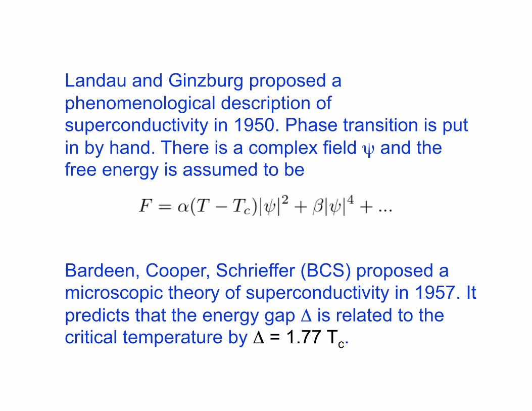
Landau and Ginzburg proposed a phenomenological description of superconductivity in 1950. Phase transition is put in by hand. There is a complex field ψ and the free energy is assumed to be

Bardeen, Cooper, Schrieffer (BCS) proposed a microscopic theory of superconductivity in 1957. It predicts that the energy gap Δ is related to the critical temperature by Δ = 1.77 Tc.

The electron-phonon interaction is weak, and Cooper pairs are much larger than the interatomic spacing.

It was once thought that the highest Tc for a BCS superconductor was around 30o K. But in 2001, MgB2 was found to be superconducting at 40o K and is believed to be described by BCS. Some people now speculate that BCS could describe a superconductor with Tc = 200o.

The new high Tc superconductors were discovered in 1986. These cuprates (e.g. YBaCuO) are layered and superconductivity is along CuO2 planes.

Highest Tc today (HgBaCuO) is Tc = 134K.

Another class of superconductors discovered March 08 based on iron and not copper FeAs(…) Highest Tc = 56K.

The pairing mechanism is not well understood. Unlike BCS theory, it involves strong coupling.

AdS/CFT is an ideal tool to study strongly coupled field theories.

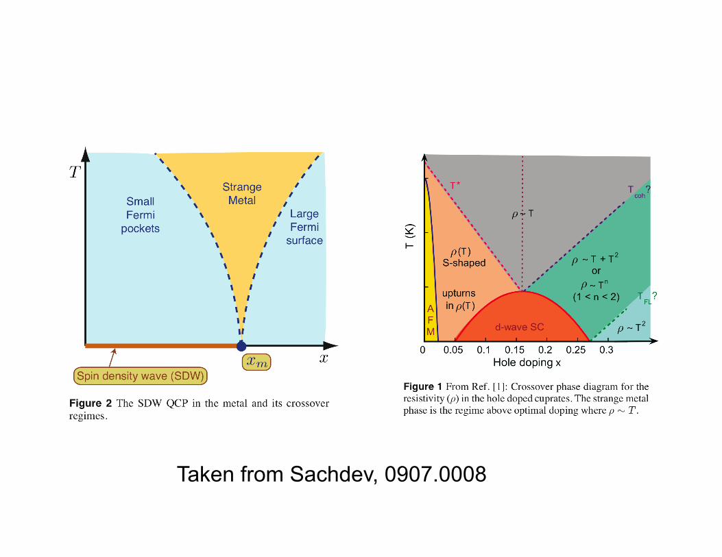
Taken from Sachdev, 0907.0008

AdS/CFT Dictionary

Gravity Superconductor

Black hole Temperature

Charged scalar field Condensate

Need to find a black hole that has scalar hair at low temperatures, but no hair at high temperatures.

This is not an easy task.

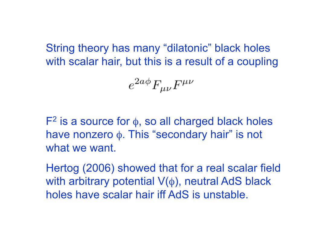
String theory has many “dilatonic” black holes with scalar hair, but this is a result of a coupling

F2 is a source for φ, so all charged black holes have nonzero φ. This “secondary hair” is not what we want.

Hertog (2006) showed that for a real scalar field with arbitrary potential V(φ), neutral AdS black holes have scalar hair iff AdS is unstable.

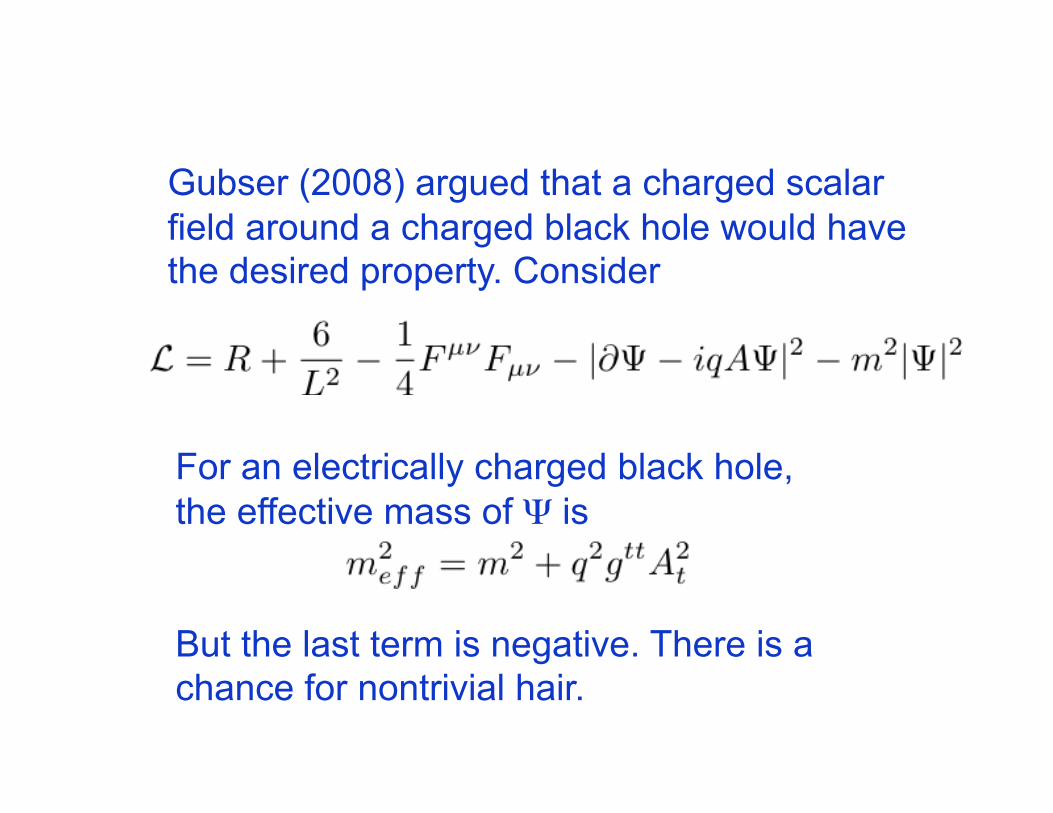
Gubser (2008) argued that a charged scalar field around a charged black hole would have the desired property. Consider

For an electrically charged black hole, the effective mass of Ψ is

But the last term is negative. There is a chance for nontrivial hair.

Quantum picture: If qQ is large enough, even extremal black holes create pairs of charged particles. In AdS, the charged particles can’t escape, and settle outside the horizon.

Qi Qf<Qi Qf<Qi

Scalar field with charge Qi - Qf

This does not work for asymptotically flat spacetimes, but does work for asymptotically AdS spacetimes.

If you rescale A A/q and Ψ Ψ /q, then the matter action has a 1/q2 in front, so that large q suppresses the backreaction on the metric.

We will first consider this large q (probe) limit for a 2+1 dimensional superconductor (four dimensional bulk). Then we will generalize to other cases.

Probe Limit

We use the planar neutral black hole

where

Hawking temperature

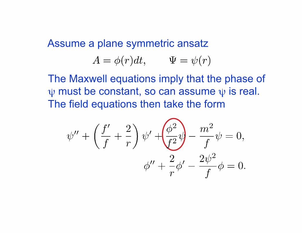
Assume a plane symmetric ansatz

The Maxwell equations imply that the phase of ψ must be constant, so can assume ψ is real. The field equations then take the form

We first consider the case m2 = - 2/L2.

Although the mass squared is negative, it is above the Breitenlohner-Freedman bound and hence does not induce an instability. It arises in several contexts in which the AdS4/CFT3 correspondence is embedded into string theory.

The source for Maxwell’s equations includes a term |ψ|2 Aµ.

At the horizon where f(r0) = 0, ϕ must vanish in order for A = ϕ dt to have finite norm. The field equations then implies that ψ and ψ’ are not independent.

So there are a two parameter family of solutions with regular horizons labeled by ϕ’(r0), ψ(r0).

Boundary conditions

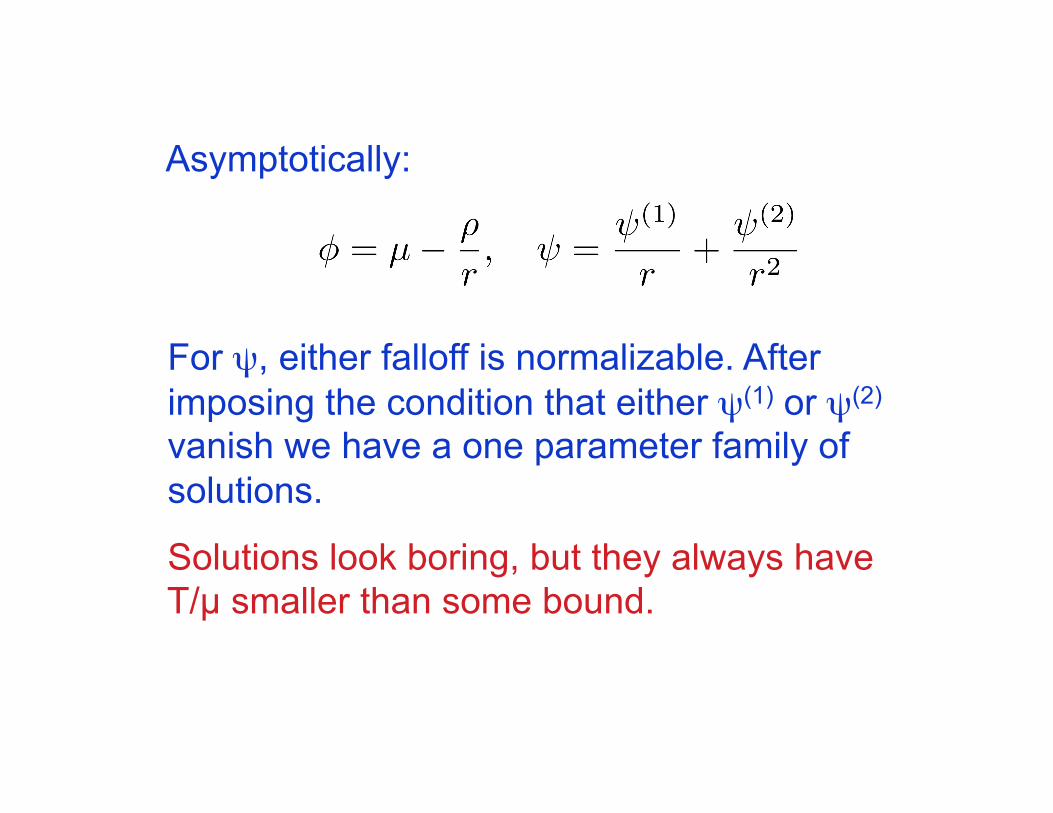
Asymptotically:

For ψ, either falloff is normalizable. After imposing the condition that either ψ(1) or ψ(2)

vanish we have a one parameter family of solutions.

Solutions look boring, but they always have T/µ smaller than some bound.

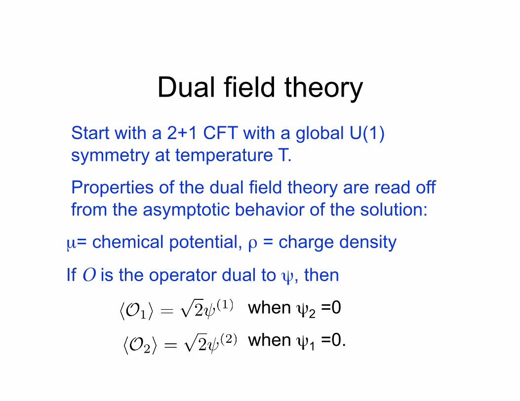
Dual field theory Start with a 2+1 CFT with a global U(1) symmetry at temperature T.

Properties of the dual field theory are read off from the asymptotic behavior of the solution:

µ = chemical potential, ρ = charge density

If O is the operator dual to ψ, then

when ψ2 =0

when ψ1 =0.

Oi has dimension i, and µ has dimension one, so Oi / Ti and T/µ are dimensionless.

Condensate (hair) as a function of T

Near the transition, there is a square root behavior

One can compute the free energy (euclidean action) of these hairy configurations and compare with the solution ψ = 0, ϕ = µ - ρ/r. The free energy is always lower for the hairy configurations and becomes equal as T→Tc.

This is a second order phase transition.

Generalize to other dimensions and other masses

We use the planar neutral black hole (i = 1,…,d-1)

where

Hawking temperature

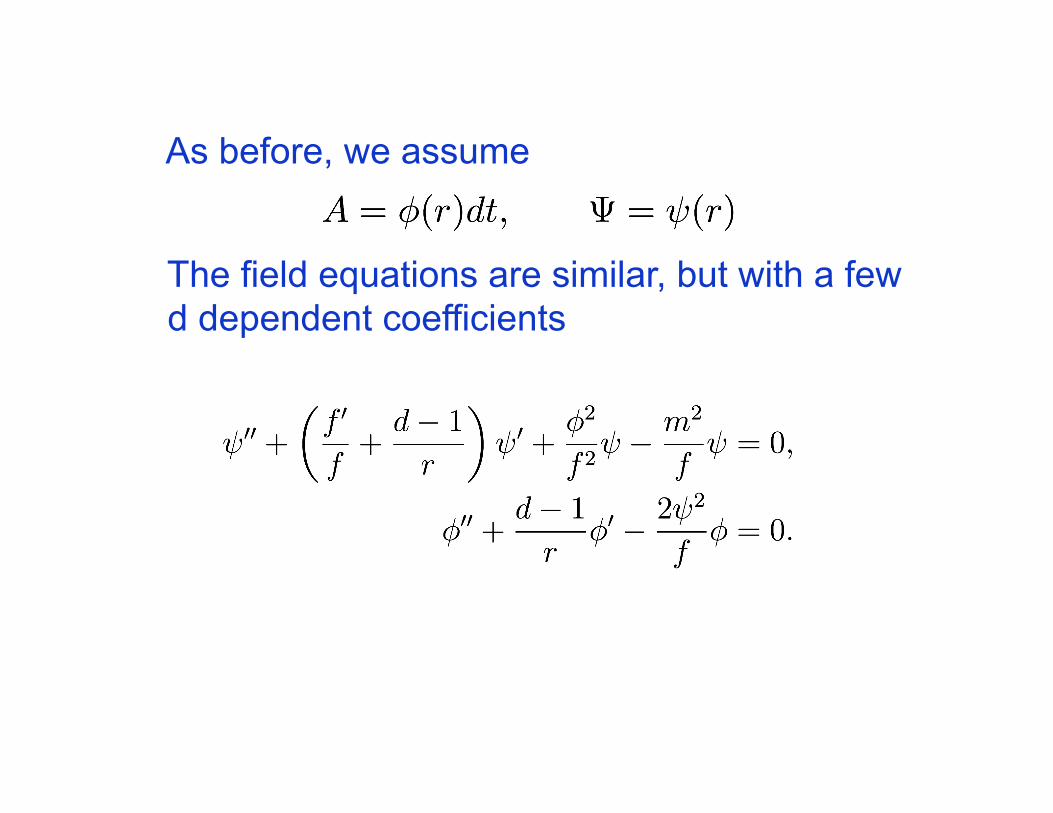
As before, we assume

The field equations are similar, but with a few d dependent coefficients

Asymptotically:

where

Typically, we need to impose ψ- = 0, in order for ψ to be normalizable. This gives a one parameter family of solutions.

If O is the operator dual to ψ, then O has dimension λ+ and

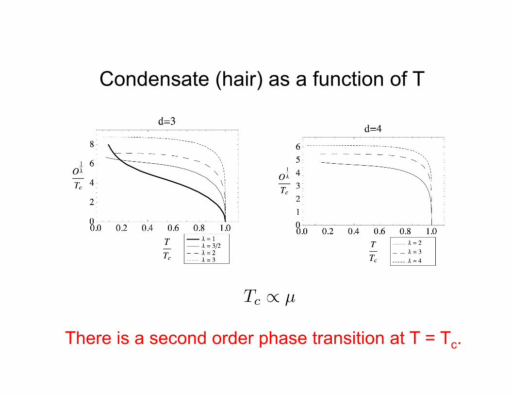
Condensate (hair) as a function of T

There is a second order phase transition at T = Tc.

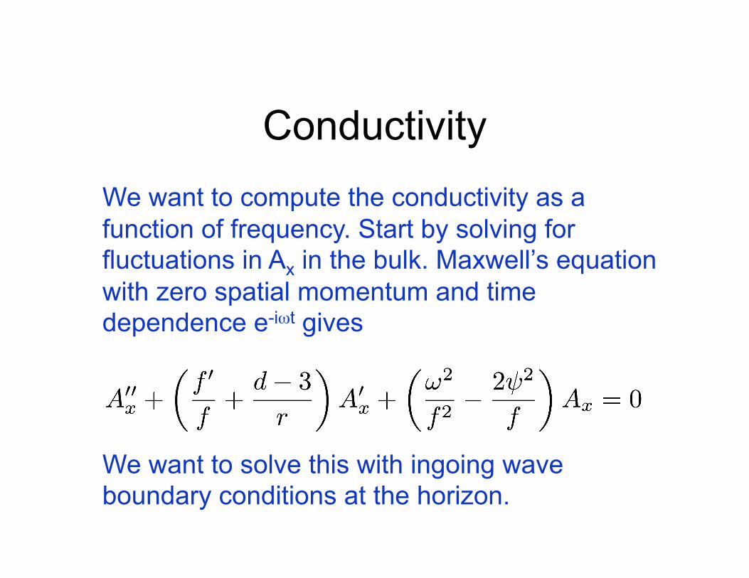
Conductivity We want to compute the conductivity as a function of frequency. Start by solving for fluctuations in Ax in the bulk. Maxwell’s equation with zero spatial momentum and time dependence e-iωt gives

We want to solve this with ingoing wave boundary conditions at the horizon.

For d = 3, the asymptotic behavior is

The AdS/CFT dictionary says

From Ohm’s law we obtain the conductivity

O1 O2

Curves represent successively lower temperatures. Gap opens up for T < Tc.

Consider first λ = 1, 2 (d = 3)

There is a delta function at ω = 0 for all T < Tc.

This can be seen by looking for a pole in Im[σ].

Simple derivation (Drude model):

If E(t) = Ee-iωt, where k=ne2/m

So

For superconductors, τ→∞,

More general derivation: The Kramers-Kronig relations relate the real and imaginary parts of any causal quantity, such as the conductivity, when expressed in frequency space.

So the real part of the conductivity contains a delta function if and only if the imaginary part has a pole. One indeed finds a pole in Im[σ] at ω = 0 for all T < Tc.

Low temperature limit of conductivity

Solid line is real part. Dashed line is imaginary part.

If the BF bound is saturated, something interesting happens.

As you lower T, a new spike appears inside the gap. This looks like a new bound state of quasiparticles.

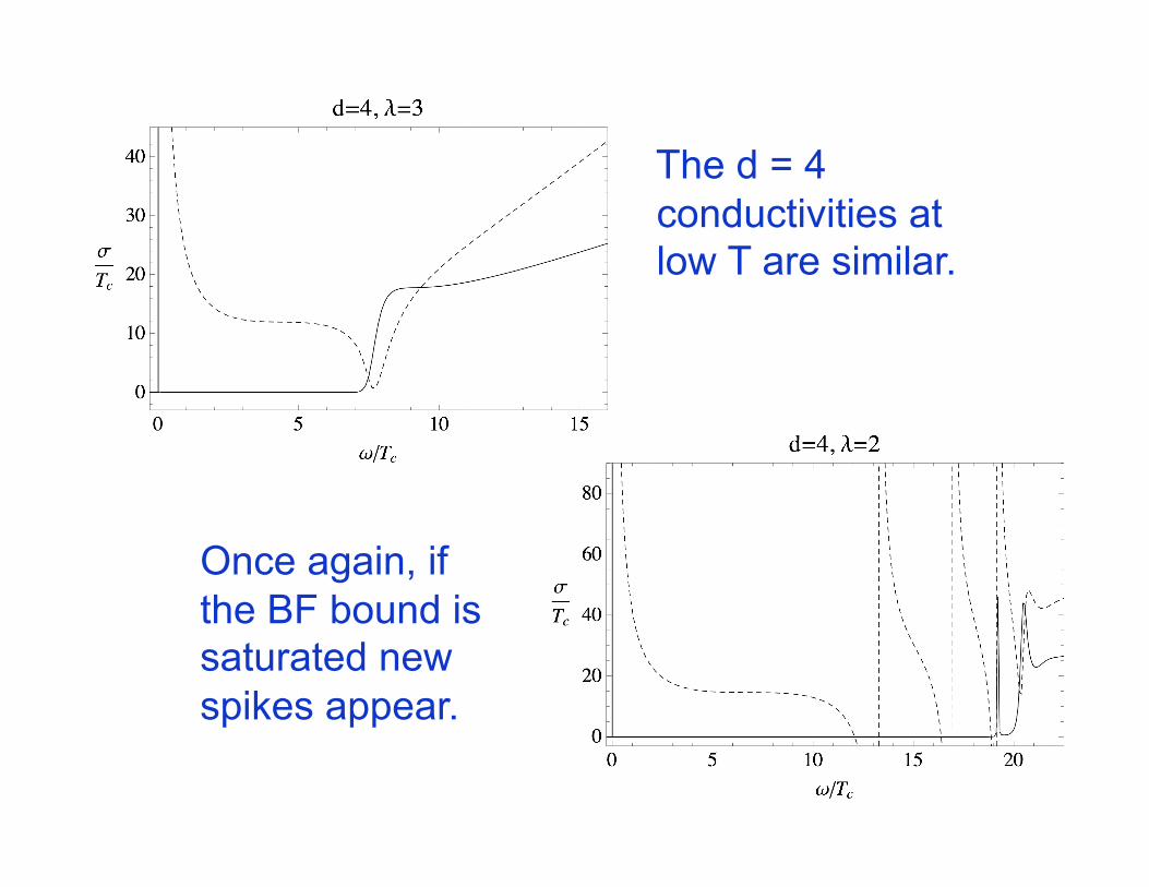
The d = 4 conductivities at low T are similar.

Once again, if the BF bound is saturated new spikes appear.

A robust feature

For both d=3 and d=4, and all λ > λBF

with deviations of less than 10%. In BCS theory, this ratio is about 3.5. This shows that the energy to break apart the condensate is more than twice the weakly coupled value. (This is modified by higher order curvature effects in bulk, Gregory et al. 0907.3203. See talk by Kanno this afternoon.)

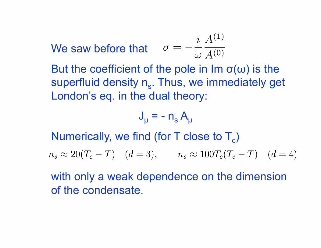
We saw before that

But the coefficient of the pole in Im σ(ω) is the superfluid density ns. Thus, we immediately get London’s eq. in the dual theory:

Jµ = - ns Aµ

Numerically, we find (for T close to Tc)

with only a weak dependence on the dimension of the condensate.

Correlation length

The retarded Green’s function (current-current two point function) is

Considering perturbations with eikx

dependence, one can define a correlation length by expanding

The d=3 correlation length. Near T = Tc:

Part 1 Summary

•  A simple gravitational theory can reproduce basic properties of a superconductor in both d=3 and d=4 spacetime dimensions.

•  When λ = λBF, new spikes appear in Re σ(ω).

•  When λ > λBF; ωg/Tc ≈ 8 in all cases.

Including backreaction

Recall that our Lagrangian is

To solve for the backreaction on the metric, set

Get four coupled nonlinear ODE’s. At the horizon, r = r0, g vanishes and χ is constant.

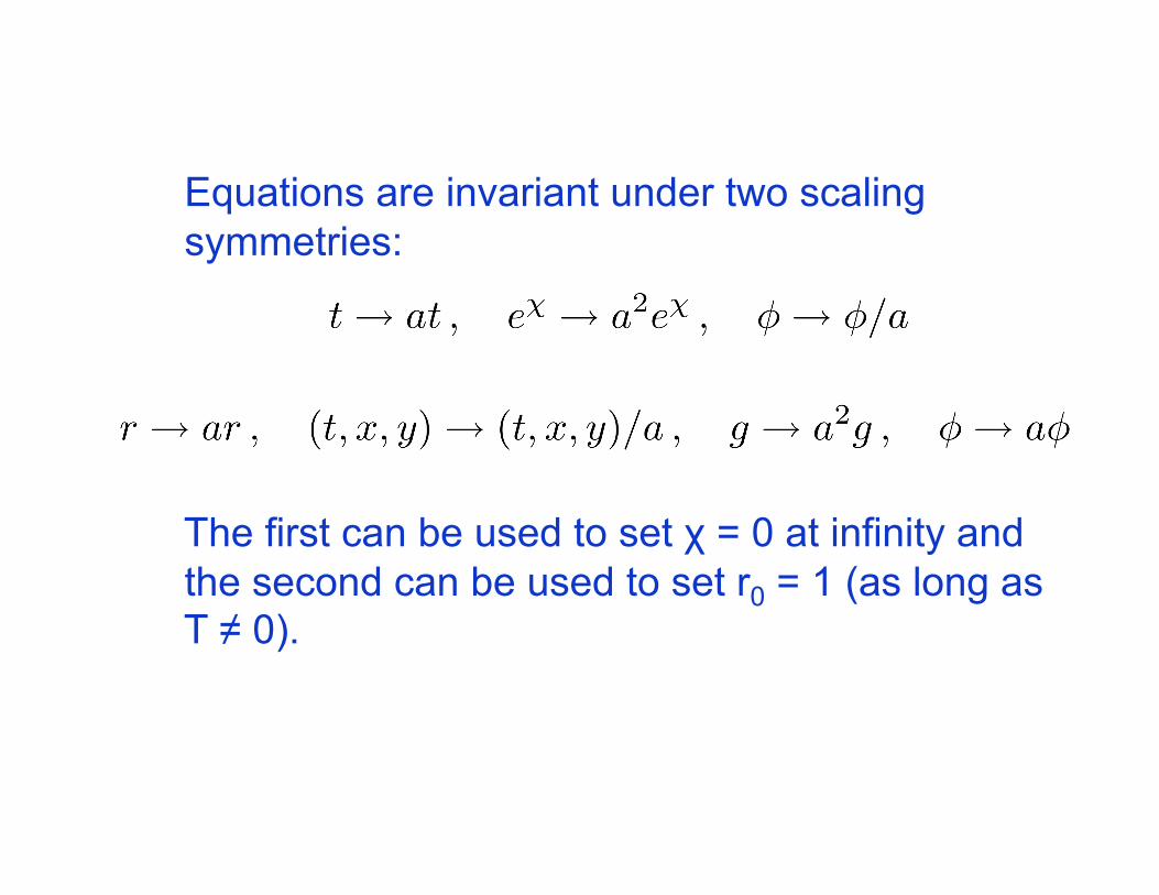
Equations are invariant under two scaling symmetries:

The first can be used to set χ = 0 at infinity and the second can be used to set r0 = 1 (as long as T ≠ 0).

We have solved the bulk equations for finite q, including the backreaction on the metric for d = 3, and various m2 ≤ 0.

The qualitative behavior is unchanged (but the “robust feature” is less robust for q < 3).

There are two main differences.

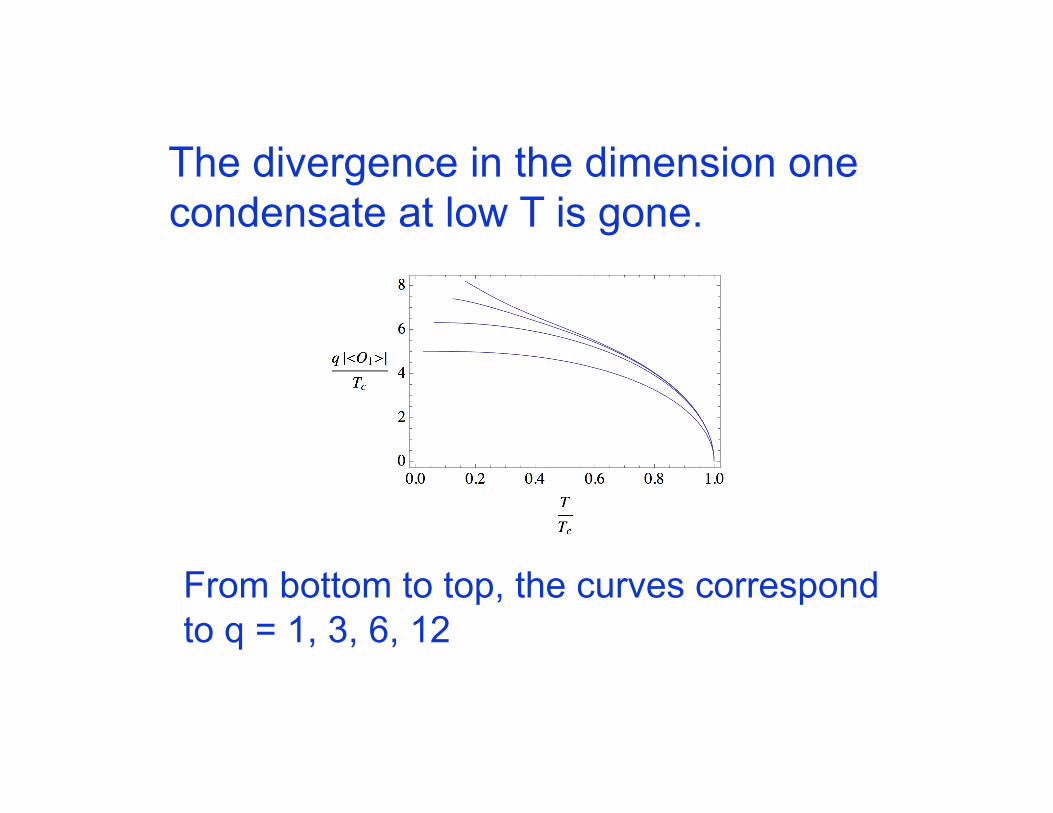
The divergence in the dimension one condensate at low T is gone.

From bottom to top, the curves correspond to q = 1, 3, 6, 12

For m2 close to BF bound, Tc remains nonzero even when q=0

There is a new source of instability: nearly extremal charged AdS black holes are unstable to forming neutral scalar hair.

An extremal AdS black hole has a near horizon geometry AdS2 x R2. The BF bound for AdSd+1 is m2

BF = - d2/4. Our scalar can be above the BF bound for AdS4, but below the bound for AdS2.

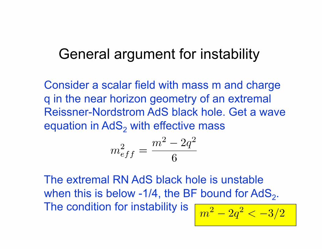
General argument for instability

Consider a scalar field with mass m and charge q in the near horizon geometry of an extremal Reissner-Nordstrom AdS black hole. Get a wave equation in AdS2 with effective mass

The extremal RN AdS black hole is unstable when this is below -1/4, the BF bound for AdS2. The condition for instability is

Conductivity

The perturbed Maxwell field Ax now couples to the perturbed metric component gtx. One can solve for gtx in terms of Ax and get

If The conductivity is again

Reformulation of Conductivity Calculation

Introduce a new radial variable

Near the horizon and asymptotically

The equation for the perturbed vector potential takes the form of a standard Schrodinger equation

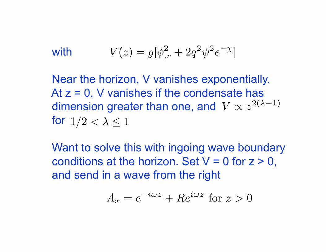
with

Near the horizon, V vanishes exponentially. At z = 0, V vanishes if the condensate has dimension greater than one, and for

Want to solve this with ingoing wave boundary conditions at the horizon. Set V = 0 for z > 0, and send in a wave from the right

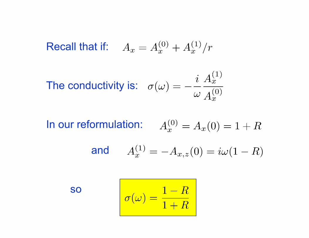
Recall that if:

The conductivity is:

In our reformulation:

and

so

The potential grows as T/Tc gets smaller (for q= 10, λ = 2)

To see the delta function in Re σ at ω = 0, we need to have a pole in Im σ. From

it suffices that Ax(0) and Ax

(1) are real and nonzero at ω = 0. This is true for any positive V(z) that vanishes at the horizon:

If ω = 0, Schrodinger’s eq. implies Ax,zz > 0. So starting with Ax =1 at z = - ∞, and integrating to z =0, Ax

(0) and Ax(1) are indeed

real and nonzero.

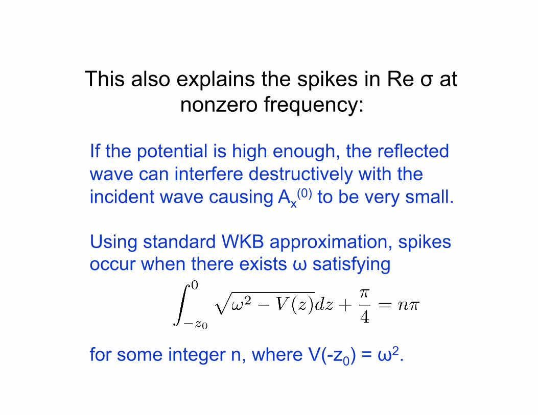
This also explains the spikes in Re σ at nonzero frequency:

If the potential is high enough, the reflected wave can interfere destructively with the incident wave causing Ax

(0) to be very small.

Using standard WKB approximation, spikes occur when there exists ω satisfying

for some integer n, where V(-z0) = ω2.

Ground State of Holographic Superconductors

The extremal Reissner Nordstrom AdS black hole has large entropy and T =0. If this was dual to a condensed matter system, it would mean the ground state was highly degenerate.

The extremal limit of the hairy black holes is not like Reissner Nordstrom. It has zero horizon area (r0/µ 0 as T 0). It also has zero charge (except when q=0).

The near horizon behavior depends on m, q. Typically, the solution is not smooth at r = 0.

Schrodinger potential still vanishes at the horizon, so Re σ(ω) ≠ 0 at low frequency even at T = 0. There is no hard gap.

Typically, V = c/z2 near the horizon, so

Re σ(ω) vanishes at T = 0 as ω 0.

Case 1: m = 0 and q2 > 3/4

Recall:

The near horizon solution is given by

The coefficients are functions of q and α. The exponent α is chosen to satisfy the boundary condition at infinity.

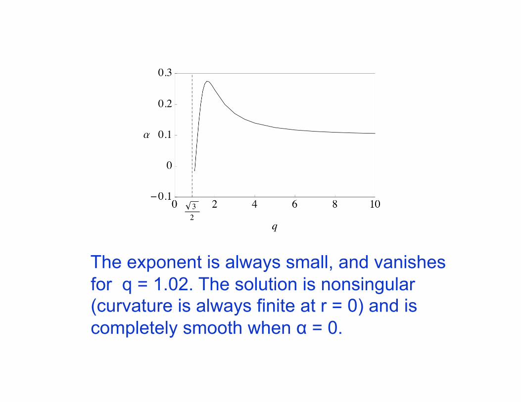
The exponent is always small, and vanishes for q = 1.02. The solution is nonsingular (curvature is always finite at r = 0) and is completely smooth when α = 0.

Low temperature solutions approach T=0 solution.

Dotted blue curve is T=0 solution with q=1. Black curves are successively lower temperature solutions.

These solutions approach AdS4 near r = 0 (with the same value of the cosmological constant as infinity).

The holographic superconductor has emergent conformal symmetry in the infrared.

The bulk solutions describe charged scalar solitons.

Case 2: m2 < 0, q2 > |m2|/6

The near horizon solution is given by

β is a fixed function of m and q. φ0 can be adjusted to satisfy boundary condition at infinity.

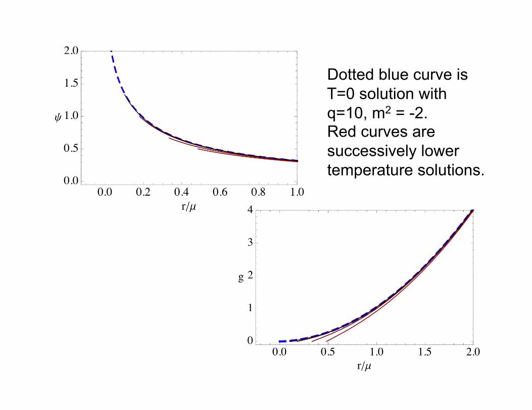
Dotted blue curve is T=0 solution with q=10, m2 = -2. Red curves are successively lower temperature solutions.

Near r = 0, the metric takes the form

There is a mild null singularity.

The holographic superconductor has emergent Poincare symmetry (but not conformal symmetry) in infrared.

Embedding in String Theory

Gubser et al. (0907.3510) realized the d = 4, m2 = -3, q=2 model in type IIB string theory.

Gauntlet et al. (0907.3796) realized the d=3, m2 = -2, q=2 model in M theory.

Both used Sasaki-Einstein compactifications, where the scalar is the size of the U(1) fibration.

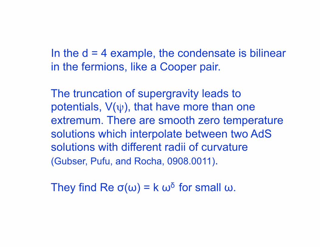
In the d = 4 example, the condensate is bilinear in the fermions, like a Cooper pair.

The truncation of supergravity leads to potentials, V(ψ), that have more than one extremum. There are smooth zero temperature solutions which interpolate between two AdS solutions with different radii of curvature (Gubser, Pufu, and Rocha, 0908.0011).

They find Re σ(ω) = k ωδ for small ω.

Adding magnetic fields (d=3) Large B fields destroy superconductivity. Superconductors must perform work B2V/8π to expel an applied field B from volume V. The thermodynamic critical field is

where F is the free energy.

Claim: If we add a magnetic field perpendicular to our 2+1 superconductor, Bc (T) = 0.

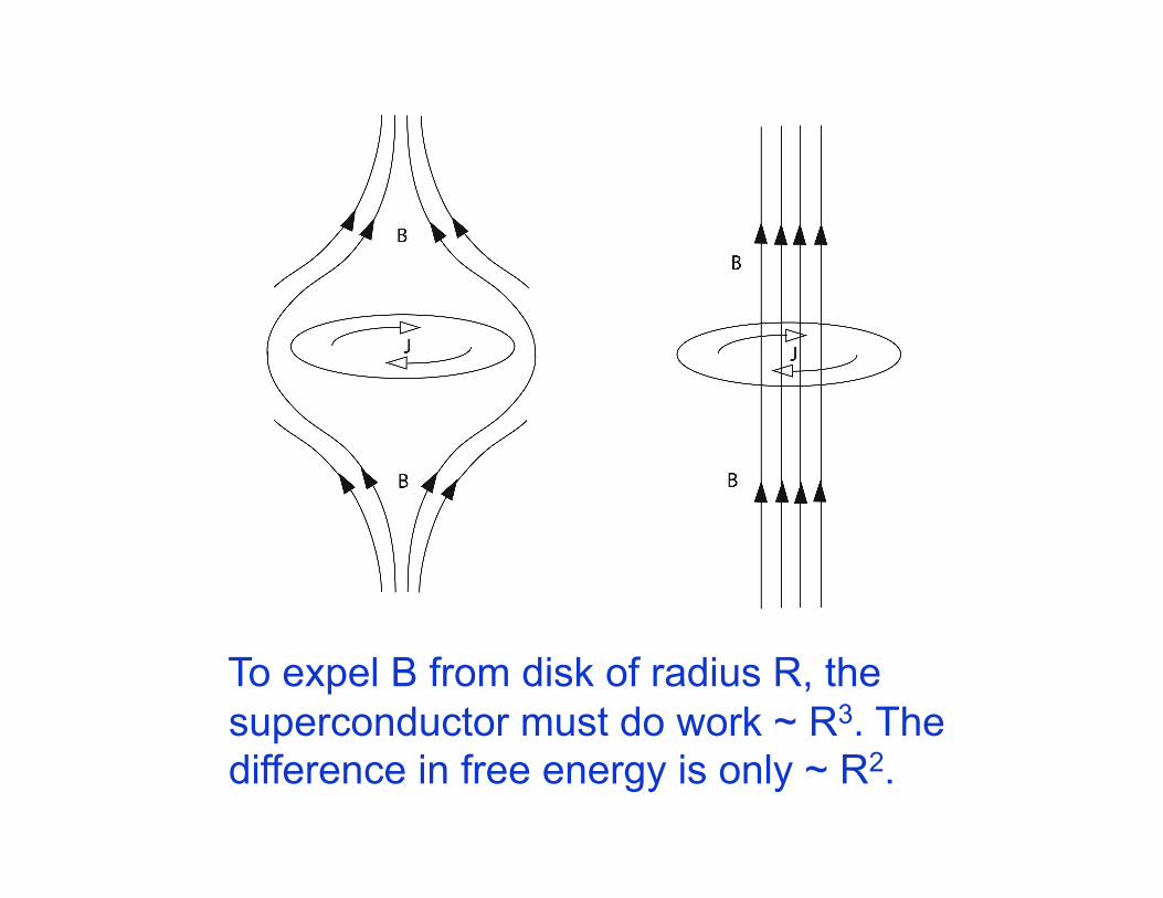
To expel B from disk of radius R, the superconductor must do work ~ R3. The difference in free energy is only ~ R2.

Starting at low T and large B, the material is in the normal phase. Now lower B.

Type I superconductors have a first order phase transition at B = Bc below which the material becomes superconducting everywhere and B = 0.

Type II superconductors have a second order phase transition at B = Bc2 > Bc where superconducting droplets form.

Holographic superconductors are Type II.

Start with Reissner-Nordstrom AdS metric with both electric and magnetic charges. Write dx2 + dy2 = du2 + u2dφ2. Then Aφ = Bu2/2.

Since we are interested in the onset of superconductivity, we can assume ψ is small. The solution takes the form ψ(r,u) = R(r) U(u).

U(u) satisfies the Schrodinger equation for a 2D harmonic oscillator, so

Numerically, we find solutions for R(r) exist for B less than a critical value Bc2 > 0.

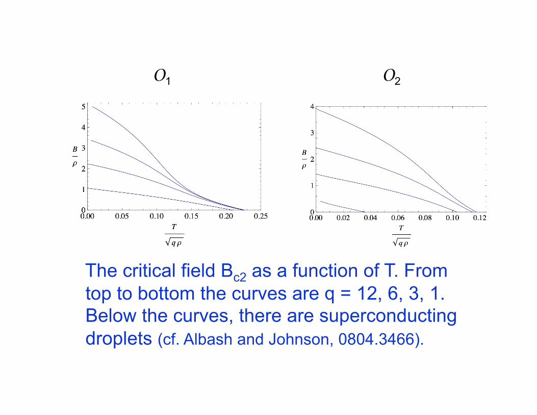
The critical field Bc2 as a function of T. From top to bottom the curves are q = 12, 6, 3, 1. Below the curves, there are superconducting droplets (cf. Albash and Johnson, 0804.3466).

O1 O2

Holographic superconductors cannot expel a B field since the U(1) symmetry is not gauged. But they do produce currents whose backreaction would cancel the B field. (see also Maeda and Okamura, 0809.3079)

The superconducting droplets generate currents around their edge. One can see this by going to second order in ψ. Find:

Aφ = Bu2/2 + Aφ(1)/r

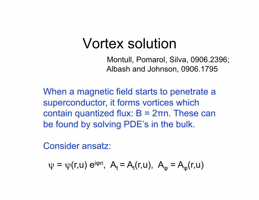
Vortex solution Montull, Pomarol, Silva, 0906.2396; Albash and Johnson, 0906.1795

When a magnetic field starts to penetrate a superconductor, it forms vortices which contain quantized flux: B = 2πn. These can be found by solving PDE’s in the bulk.

Consider ansatz:

ψ = ψ(r,u) eiφn, At = At(r,u), Aφ = Aφ(r,u)

u

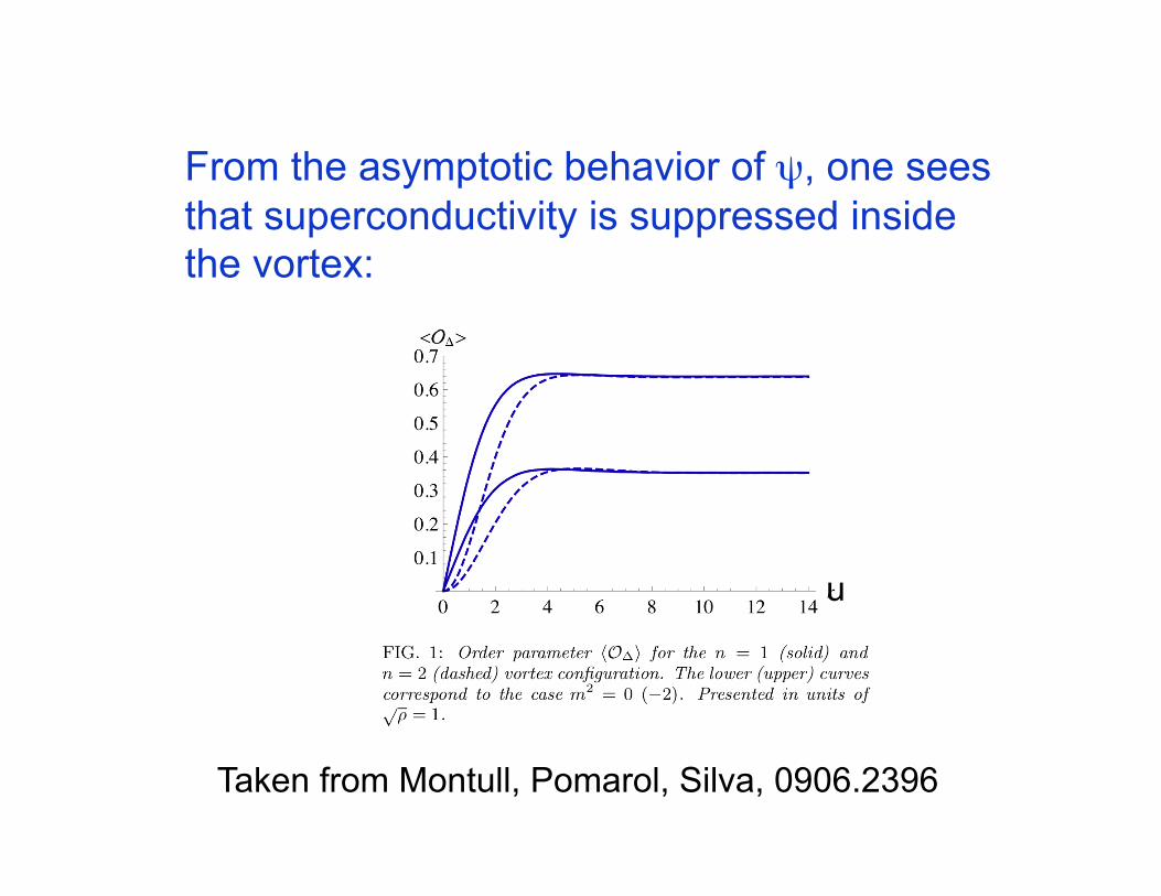
From the asymptotic behavior of ψ, one sees that superconductivity is suppressed inside the vortex:

Taken from Montull, Pomarol, Silva, 0906.2396

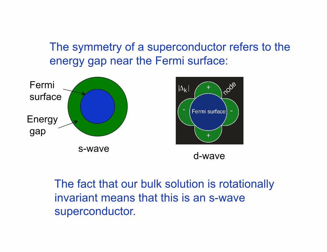
The symmetry of a superconductor refers to the energy gap near the Fermi surface:

s-wave d-wave

The fact that our bulk solution is rotationally invariant means that this is an s-wave superconductor.

Energy gap

Fermi surface

Part 2 Summary

•  There are two distinct instabilities which cause condensate (hair) to form at low T.

•  The conductivity is simply related to a reflection coefficient in a scattering problem

•  There is no hard gap (Re σ(ω) ≠ 0 at T = 0). •  Holographic superconductors are Type II.