HOLOMORPHIC FUNCTIONS AND THE HEAT KERNEL MEASURE ON AN INFINITE DIMENSIONAL COMPLEX ORTHOGONAL GROUP MARIA GORDINA Department of Mathematics, Cornell University, Ithaca, NY 14853, USA Abstract. The heat kernel measure μt is constructed on an infinite dimen- sional complex group using a diffusion in a Hilbert space. Then it is proved that holomorphic polynomials on the group are square integrable with respect to the heat kernel measure. The closure of these polynomials, L 2 (SO HS ,μt ), is one of two spaces of holomorphic functions we consider. The second space, L 2 (SO(∞)), consists of functions which are holomorphic on an analog of the Cameron-Martin subspace for the group. It is proved that there is an isometry from the first space to the second one. The main theorem is that an infinite dimensional nonlinear analog of the Taylor expansion defines an isometry from L 2 (SO(∞)) into the Hilbert space associated with a Lie algebra of the infinite dimensional group. This is an extension to infinite dimensions of an isometry of B. Driver and L. Gross for complex Lie groups. All the results of this paper are formulated for one concrete group, the Hilbert-Schmidt complex orthogonal group, though our methods can be ap- plied in more general situations. 1. Introduction In this paper we will study Hilbert spaces of holomorphic functions over a partic- ular infinite dimensional complex group G. We will choose an infinite dimensional Lie algebra naturally associated with the group, and fix a Hermitian inner product on it. As usual, one may view the universal enveloping algebra as a space of left- invariant differential operators on the group. A holomorphic function on G then determines an element, α, of the dual of the universal enveloping algebra by means of the identity hα, βi =(βf )(e) for all left-invariant differential operators β, where e is the identity element of the group. Thus, α is just the set of Taylor coefficients of f at the identity. When G is finite dimensional, the Taylor map, f 7→ α, is known (cf. [7]) to be an isometry from the Hilbert space of holomorphic functions, square integrable with respect to a heat kernel measure on G, to a subspace of the dual of the universal enveloping algebra. An outline of these finite dimensional results of B. Driver and L. Gross [7] will be given later in the introduction. The objective of the present work is to establish a corresponding isometry for an infinite dimensional group. 1991 Mathematics Subject Classification. Primary 46E50, 60H15; Secondary 22E30, 22E65, 58G32. Key words and phrases. Heat kernel measure, infinite dimensional group, stochastic differential equation. 1
Transcript
HOLOMORPHIC FUNCTIONS AND THE HEAT KERNELMEASURE ON AN INFINITE DIMENSIONAL COMPLEX
ORTHOGONAL GROUP
MARIA GORDINADepartment of Mathematics, Cornell University, Ithaca, NY 14853, USA
Abstract. The heat kernel measure µt is constructed on an infinite dimen-sional complex group using a diffusion in a Hilbert space. Then it is provedthat holomorphic polynomials on the group are square integrable with respectto the heat kernel measure. The closure of these polynomials, HL2(SOHS , µt),is one of two spaces of holomorphic functions we consider. The second space,HL2(SO(∞)), consists of functions which are holomorphic on an analog of theCameron-Martin subspace for the group. It is proved that there is an isometryfrom the first space to the second one.
The main theorem is that an infinite dimensional nonlinear analog of theTaylor expansion defines an isometry fromHL2(SO(∞)) into the Hilbert spaceassociated with a Lie algebra of the infinite dimensional group. This is anextension to infinite dimensions of an isometry of B. Driver and L. Gross forcomplex Lie groups.
All the results of this paper are formulated for one concrete group, theHilbert-Schmidt complex orthogonal group, though our methods can be ap-plied in more general situations.
1. Introduction
In this paper we will study Hilbert spaces of holomorphic functions over a partic-ular infinite dimensional complex group G. We will choose an infinite dimensionalLie algebra naturally associated with the group, and fix a Hermitian inner producton it. As usual, one may view the universal enveloping algebra as a space of left-invariant differential operators on the group. A holomorphic function on G thendetermines an element, α, of the dual of the universal enveloping algebra by meansof the identity 〈α, β〉 = (βf)(e) for all left-invariant differential operators β, wheree is the identity element of the group. Thus, α is just the set of Taylor coefficientsof f at the identity. When G is finite dimensional, the Taylor map, f 7→ α, is known(cf. [7]) to be an isometry from the Hilbert space of holomorphic functions, squareintegrable with respect to a heat kernel measure on G, to a subspace of the dual ofthe universal enveloping algebra. An outline of these finite dimensional results ofB. Driver and L. Gross [7] will be given later in the introduction. The objective ofthe present work is to establish a corresponding isometry for an infinite dimensionalgroup.
Key words and phrases. Heat kernel measure, infinite dimensional group, stochastic differentialequation.
1
2 MARIA GORDINA
Two fundamental differences between the finite dimensional and infinite dimen-sional cases must be addressed. First, we need to have an analog of the heat kernelmeasure on an infinite dimensional, non locally compact, non commutative group.For a finite dimensional group the heat kernel measure has a density with respectto Haar measure, making it possible to apply techniques from partial differentialequations. However, on the group to be considered in this paper there is no Haarmeasure to help analyze a heat kernel density. Partial differential equation tech-niques for studying such measures are not available. Instead, we will use stochasticdifferential equations in infinite dimensions to construct such a measure. The the-ory of such equations has been developed for Hilbert and Banach spaces, not infinitedimensional manifolds or groups. Moreover, since there are no previous examples toguide our intuition for a general theory, we will focus in this paper on one particularcase. We will take the group to be the group of complex Hilbert-Schmidt orthogonaloperators over an infinite dimensional Hilbert space. This Hilbert-Schmidt complexorthogonal group, SOHS , will be described in Section 2. The fact that the groupSOHS can be embedded in a Hilbert space, namely, the space of Hilbert-Schmidtoperators, plays an important role in the construction of the heat kernel measure.To construct the heat kernel measure we will use a diffusion on the group. We willconstruct the diffusion on G by first constructing a diffusion on this ambient Hilbertspace. The stochastic differential equation determining the diffusion is nonlinearwith Lipshitz nonlinearities, and its coefficients are chosen in such a way that thestochastic process actually lives in the group. Then we will use finite dimensionalapproximations to this diffusion to obtain some of our results. We can identifyelements of the group with infinite matrices, which allows us to make significantuse of the polynomials in the matrix entries. Using properties of the stochastic pro-cess we will prove that these naturally defined holomorphic polynomials are squareintegrable with respect to the measure determined by the process.
A second difference between the finite and infinite dimensional cases arises fromthe need to find a viable notion of holomorphic function on the group SOHS . We willconsider two spaces of holomorphic functions. One of the spaces,HL2(SOHS , µt), is defined as the closure of the holomorphic polynomials inL2(µt)-norm. However, such a function might not have a version which is differen-tiable on the whole group. Therefore we also consider a Hilbert space HL2(SO(∞))of functions differentiable on a subset SO(∞) of the group. This subset plays therole of the Cameron-Martin subspace. The main theorem is that the Taylor map,f 7→ α, is an isometry from HL2(SO(∞)) into a Hilbert space contained in the dualof the universal enveloping algebra. This will imply, in particular, that any functionin HL2(SO(∞)) is uniquely determined by its derivatives at the identity. In addi-tion, there is a natural isometry from the closure of the holomorphic polynomialsin L2(µt)-norm to HL2(SO(∞)). This isometry is an extension of the inclusion ofthese polynomials into this second space.
When G is finite dimensional, the heat kernel measure is defined as follows. Thereis a unique probability measure satisfying et∆/4f = µt ∗ f, where the Laplacian ∆is a naturally defined second order differential operator associated with a givenHermitian inner product on the Lie algebra of G. In the finite dimensional case themeasure µt = µt(z)dz has the heat kernel µt(z) as its density with respect to Haarmeasure on G. Note that if G = Cn then the heat kernel measure µt is a Gaussianmeasure. Denote by HL2(G,µt(z)dz) the space of holomorphic functions over Gwhich are square integrable with respect to the heat kernel measure µt. B. Driver
HOLOMORPHIC FUNCTIONS ON AN INFINITE DIMENSIONAL GROUP 3
and L. Gross [7] have shown that the Taylor map, f 7→ α, is an isomorphismbetween HL2(G,µt(z)dz) and a subspace, J0
t , of the algebraic dual of the universalenveloping algebra of the Lie algebra of G, when G is a connected simply connectedcomplex (finite dimensional) Lie group. J0
t is a Hilbert space with respect to a normwhich is naturally associated with the given inner product on the Lie algebra of G.
In finite dimensions, when G happens to be the complexification of a compactLie group K, there is, in addition to the two Hilbert spaces, HL2(G,µt(z)dz)and J0
t , discussed above, a third naturally arising Hilbert space. The third spaceis L2(K, ρt(x)dx), where ρt(x)dx is the heat kernel measure associated to a bi-invariant Laplacian on K. B. Hall [11], [12] has described a natural unitary iso-morphism from L2(K, ρt(x)dx) to HL2(G, µt(z)dz). It is worth noting that oneshould not expect an analog of Hall’s transform for our group because his proofrequires Ad-invariance of the inner product on Lie(K), and this condition seemsto be really essential. By contrast, the isomorphism from HL2(G,µt(z)dz) to J0
tdoes not require Ad-invariance of the Hermitian inner product on the Lie algebraof G. This is important in infinite dimensions since the norm we need to use isnot Ad-invariant. Though there is an invariant inner product on the Lie algebraof SOHS , namely, the Hilbert-Schmidt inner product, J0
t turns out to be trivial inthis case. The same happens for some other infinite dimensional groups whose Liealgebras have Ad-invariant inner product. We will show this in Section 8 for theHilbert-Schmidt complex orthogonal group, SOHS .
L. Gross proved in [9] the isomorphism between L2(K, ρt(x)dx) and J0t for a
compact connected Lie group K using probabilistic methods. Later O. Hijab in[14], [15] found an analytical proof of this isomorphism. This isometry also de-pends on the AdK-invariance of the inner product on Lie(K) and seems unlikelyto have a natural analog for our infinite dimensional orthogonal group. An extensiveexposition of the subject can be found in [10].
In conclusion, we should note that in the case when G is replaced by a separableHilbert space, J0
t is a bosonic Fock space. In this situation the isomorphismsbetween these three spaces give three different representations of the Fock space.The isomorphisms were studied by V.Bargmann, I. Segal, P. Kree and others (see,for example, [1], [2], [17], [24], [25]). Recently such spaces have been studied in caseof a complex abstract Wiener space by several authors including I. Shigekawa [26]and H. Sugita [28], [29]. Our results are precise analogs of some of the linear resultsof I. Shigekawa and H. Sugita, though the methods are entirely different.
Not much is known for infinite dimensional groups. However, B. Hall and A. Sen-gupta [13] have extended the isomorphism between L2(K, ρt(x)dx) andHL2(G,µt(x)dx) to the group of paths in a compact (finite dimensional) Lie group.
There have been a number of works about properties of infinite dimensionalorthogonal and unitary groups. The representation theory of these groups hasbeen studied, for example, in [16], [20], [27]. P. da la Harpe, R.J. Plymen andR.F. Streater have described topological properties of infinite dimensional orthog-onal groups in [4], [5], [19] in connection with spinors in Hilbert space. One of thegroups they have considered is the Hilbert-Schmidt orthogonal group.
Acknowledgement. I wish to thank Professor L. Gross for his invaluable guid-ance throughout the process of preparation of this work. It is a pleasure to acknowl-edge stimulating discussions with Professor E. Dynkin and Professor B. Driver.
4 MARIA GORDINA
2. Notation and main results
First of all, we describe the group we will consider in this paper. This group isrepresented as a group of operators in a Hilbert space. Let Hr be a real separableHilbert space, H = Hr⊕ iHr its complexification and I the identity operator on H.Denote by HSr the Hilbert-Schmidt operators on Hr. Then HSr is a real Hilbertspace equipped with the Hilbert-Schmidt inner product 〈A, B〉HSr = Tr(B∗A) forany A, B ∈ HSr.
Consider the complexification of HSr denoted by HS = HSr ⊕ iHSr. HS canbe identified with the space of complex linear Hilbert-Schmidt operators on H.Any element A ∈ HS can be written as a sum of ReA and i ImA, where ReA andImA ∈ HSr. The product of elements of HS is defined naturally by
AB = (ReA ReB − ImA ImB) + i (ReA ImB + ImA ReB).
The space HS is a real Hilbert space equipped with the following inner product:
Definition 2.1. The Hilbert-Schmidt complex orthogonal group SOHS is the con-nected component containing the identity I of the group OHS = B : B − I ∈HS, BT B = BBT = I, where BT means the transpose of the operator B, i. e.BT = (ReB)∗ + i(ImB)∗.
Proposition 4.4 shows why OHS is not connected. The fact that SOHS−I ⊂ HSgives two essential advantages: first of all, it helps to define an inner product on a Liealgebra of SOHS , and second, it will allow us to construct the heat kernel measureon SOHS . The Lie algebra of skew-symmetric Hilbert-Schmidt operators soHS =A : A ∈ HS,AT = −A plays the role of a Lie algebra of SOHS . The group SOHSis the complexification of the Hilbert-Schmidt orthogonal group, SOHSr , and soHS
is the complexification of its Lie algebra. Note that 〈·, ·〉HS is an Ad-HSr-invariantinner product on soHS . Later we will consider another inner product on a densesubspace of soHS (which is not Ad-invariant) since the isometry we are trying toestablish is trivial in the invariant case.
We will consider three Hilbert spaces HL2(SOHS , µt), HL2(SO(∞)) and J0t .
The first two spaces are spaces of functions, while J0t has an algebraic nature.
The first space, HL2(SOHS , µt), is the closure in L2(SOHS , µt) of the space ofholomorphic polynomials (in the matrix entries) on SOHS . Here µt is the heat ker-nel measure on SOHS which will be defined in Section 3 as the transition probabilityof a diffusion on SOHS . Note that this definition uses the fact that all holomorphicpolynomials are square-integrable with respect to the heat kernel measure. Thelatter will be proved in Section 5.
To define HL2(SO(∞)) we consider SO(∞), a subset of SOHS , which is theclosure of the direct limit of a sequence of finite dimensional subgroups of SOHS
in a Riemannian metric. More precisely, fix an orthonormal basis fm∞m=1 of Hr.Let HSn×n = A : 〈Afm, fk〉 = 0 if max(m, k) > n. Take a basis ek∞k=1 of HSsuch that ek2n2
k=1 is a basis of HSn×n. Note that SOHS(n) = B ∈ SOHS , B−I ∈HSn×n is a group isomorphic to the complexification of the special orthogonalgroup of Rn. Then gn = Lie(SOHS(n)) = soHS(n) = A ∈ HSn×n, AT = −A isits Lie algebra. Note that g = ∪ngn is a Lie subalgebra of soHS . We will choosea new inner product 〈〈·, ·〉〉 on g so that the corresponding norm is stronger thanthe Hilbert-Schmidt norm. This new inner product defines a Riemannian metric
HOLOMORPHIC FUNCTIONS ON AN INFINITE DIMENSIONAL GROUP 5
on ∪nSOHS(n). SO(∞) is the closure of ∪nSOHS(n) in this Riemannian metric.Then HL2(SO(∞)) denotes a certain space of holomorphic functions on SO(∞)with a certain direct limit-type norm. More detailed definitions of these objects aregiven in Section 7.
Finally, we need the following notation to describe J0t .
Notation 2.2. Let g be a complex Lie algebra with a Hermitian inner product onit. Then T (g) will denote the algebraic tensor algebra over g as a complex vectorspace and T ′(g) will denote the algebraic dual of T (g). Define a norm on T (g) by
|β|2t =n
∑
k=0
k!tk|βk|2, β =
n∑
k=0
βk, βk ∈ g⊗k, k = 0, 1, 2, ..., t > 0(2.1)
Here |βk| is the cross norm on g⊗k arising from the inner product on g⊗k determinedby the given inner product on g. The coefficients k!
tk are related to the heat kernel.Tt(g) will denote the completion of T in this norm. The topological dual of Tt(g)may be identified with the subspace T ∗t (g) of T ′(g) consisting of such α ∈ T ′(g) thatthe norm
|α|2t =∞∑
k=0
tk
k!|αk|2, α =
∞∑
k=0
αk, αk ∈ (g⊗k)∗, k = 0, 1, 2, ..., t > 0(2.2)
is finite. Here |αk| is the norm on (g⊗k)∗ dual to the cross norm on g⊗k.There is a natural pairing for any α ∈ T ′(g) and β ∈ T (g) denoted by
〈α, β〉 =∞∑
k=0
〈αk, βk〉, α =∞∑
k=0
αk, β =n
∑
k=0
βk, αk ∈ (g⊗k)∗, βk ∈ g⊗k, k = 0, 1, 2, ...
Denote by J(g) the two-sided ideal in T (g) generated by ξ⊗η−η⊗ξ−[ξ, η], ξ, η ∈ g.Let J0(g) = α ∈ T ′(g) : α(J) = 0. Finally, let J0
t (g) = T ∗t (g) ∩ J0(g).
The first natural choice for g for our group is soHS with the Hilbert-Schmidtinner product, which is Ad-HSr-invariant. The problem with this inner productis that in this case J0
t is trivial (see Section 8). Therefore we will use another Liealgebra, g = ∪gn = ∪soHS(n), as described above together with an appropriateinner product on g.
The inner product on g will be non Ad-invariant. Namely, the inner productis defined by 〈〈A, B〉〉 = 〈Q−1/2A,Q−1/2B〉HS , where Q is a symmetric positivetrace class operator on soHS such that all soHS(n) are invariant subspaces of Q.Actually, the closure of g in the corresponding norm is the subspace of soHS definedas U0 = Q1/2(soHS). This norm is denoted by ‖X‖U0 = ‖Q−1/2X‖HS .
In some sense U0 determines the directions in which derivatives of functions onSOHS will be taken. If we choose too large a set of directions we might not havenonconstant holomorphic functions. Moreover, if we define informally the Laplacianas
∆Q =12
∞∑
n=1
(∂ξn)2
where ξn∞n=1 is an orthonormal (in 〈〈·, ·〉〉) basis of U0, then the stronger innerproduct gives a weaker Laplacian. In Section 3.3 we show that the heat kernelmeasure µt solves the heat equation with the Laplacian ∆Q. The weaker Laplacian
6 MARIA GORDINA
allows µt to live on SOHS . Note that SO(∞) is an analog of the Cameron-Martinsubspace associated with any infinite dimensional Wiener space.
For the Lie algebra g we denote J0t = J0
t (g). The latter can be called a spaceof Taylor coefficients for functions in HL2(SO(∞)). Indeed, our main result isthat the Taylor series determines an isometry from HL2(SO(∞)) into J0
t . Thefact that J0
t is not trivial (for the Lie algebra g) follows from the existence of thisisometry from HL2(SOHS , µt) to J0
t and the fact that HL2(SOHS , µt) contains allholomorphic polynomials on SOHS .
For each function f in HL2(SO(∞)) we use a natural notation
(1−D)−1e f =
∞∑
n=1
Dne f
for the series of its derivatives at the identity considered as an element of T ′. Thenour results (Theorem 7.6, Theorem 7.5 and Theorem 7.4) can be summarized asfollows.
1. HL2(SO(∞)) is a Hilbert space.2. (1−D)−1
e is an isometry from HL2(SO(∞)) into J0t .
3. The embedding of the space of holomorphic polynomials HP into the Hilbertspace HL2(SO(∞)) can be extended to an isometry from HL2(SOHS , µt)into HL2(SO(∞)).
The following diagram describes these isometries:
HP inclusion−−−−−→ HL2(SOHS , µt)Theorem 7.4−−−−−−−−→ HL2(SO(∞)) Theorem 7.5−−−−−−−−→ J0
t
3. Construction of the heat kernel measure
The goal of this section is to define the heat kernel measure on SOHS . To achieveit we will use a diffusion on the group. If we consider a stochastic process in SOHS
Xt : Ω × R −→ SOHS , then Yt = Xt − I is an element of HS. This space is aHilbert space, which enables us to use the machinery of the stochastic differentialequations in Hilbert spaces developed in recent years.
3.1. Existence and uniqueness of a stochastic process. We begin with thedefinition of the process Yt. Denote by U the space soHS with the inner product〈·, ·〉HS . Let Wt be a U -valued Wiener process with a covariance operator Q : U −→U . We assume that Q is a symmetric positive trace-class operator. Sometimes wewill identify Q with its extension by zero to the orthogonal complement of U in HS.Let U0 = Q
12 (U) as before with the inner product 〈u, v〉0 = 〈Q−1/2u, Q−1/2v〉HS .
Denote by L02 = L2(U0,HS) the space of the Hilbert-Schmidt operators from U0
to HS with the (Hilbert-Schmidt) norm ‖Ψ‖2L02
= Tr[ΨQΨ∗].We need to define the coefficients of the stochastic differential equation before
we formulate Theorem 3.3.
Notation 3.1. B : HS −→ L02, B(Y )U = U(Y + I) for U ∈ U0, F : HS −→ HS,
F (Y ) = − 12
∑
n(Q1/2en)T (Q1/2en)(Y + I), where en∞n=1 is an orthonormal basisof HS as a real space.
Proposition 3.2.∑
m(Q1/2em)T (Q1/2em) does not depend on the choice of thebasis em∞1 . In addition,
∑
m(Q1/2em)T (Q1/2em) =∑
m eTmQem.
HOLOMORPHIC FUNCTIONS ON AN INFINITE DIMENSIONAL GROUP 7
Proof. Define a bilinear real form on HS ×HS by L(f, g) = Λ((Q1/2f)T (Q1/2g)),where Λ is a real bounded linear functional on HS. Then f 7→ L(f, g) is abounded linear functional on HS and so L(f, g) = 〈f, g〉HS for some g ∈ HS.There exists a linear operator on HS such that L(f, g) = 〈f, Bg〉HS . Now wecan see that since trace is independent of a basis, TrB =
∑
m〈em, Bem〉HS =∑
m Λ(Q1/2em)T (Q1/2em) does not depend on the choice of em∞m=1. To prove thesecond half of the statement, we note that
∑
m eTmQem is independent of em∞m=1
by similar reasons. At the same time, if we choose em∞m=1 in which Q is diagonal,say, Qem = λmem, then
∑
m(Q1/2em)T (Q1/2em) =∑
m λmeTmem =
∑
m eTmQem.
Since both sums are independent of the choice of the basis, they are equal for anybasis em∞m=1.
Theorem 3.3. 1. The stochastic differential equation
dYt = B(Yt)dWt + F (Yt)dt,
Y0 = 0(3.1)
has a unique solution, up to equivalence, among the processes satisfying
P
(
∫ T
0‖Ys‖2HSds < ∞
)
= 1.
2. For any p > 2 there exists a constant Cp,T > 0 such that
E supt∈[0,T ]
‖Yt‖pHS 6 Cp,T .
Proof of Theorem 3.3. To prove this theorem we will use Theorem 7.4, p.186 fromthe book by G.DaPrato and J.Zabczyk [3]. It is enough to check that
1. F is a measurable mapping from HS to HS.2. ‖F (Y1)− F (Y2)‖HS 6 C‖Y1 − Y2‖HS for any Y1, Y2 ∈ HS.3. ‖F (Y )‖2HS 6 K(1 + ‖Y ‖2HS) for any Y ∈ HS.4. B(Y ) is a measurable mapping from HS to L0
2.5. ‖B(Y1)−B(Y2)‖L0
26 C‖Y1 − Y2‖HS for any Y1, Y2 ∈ HS.
6. ‖B(Y )‖2L02
6 K(1 + ‖Y ‖2HS) for any Y ∈ HS.
Proof of 1. Let us check that F (Y ) is in HS for any Y ∈ HS.
‖F (Y )‖HS 612‖
∑
n
(Q1/2en)T (Q1/2en)‖HS(‖Y ‖HS + 1) < ∞,
since
‖∑
n
(Q1/2en)T (Q1/2en)‖HS 6∑
n
‖(Q1/2en)T (Q1/2en)‖HS 6
6∑
n
‖Q1/2en‖2HS = TrQ < ∞
by the assumption. The measurability is trivial.
Proof of 2.
‖F (Y1)− F (Y2)‖HS 612‖
∑
n
(Q1/2en)T Q1/2en‖HS‖Y1 − Y2‖HS 6
6 TrQ‖Y1 − Y2‖HS
8 MARIA GORDINA
as in the proof of 1.
Proof of 3.
‖F (Y )‖HS 612‖
∑
n
(Q1/2en)T (Q1/2en)Y ‖HS +
+12‖
∑
n
(Q1/2en)T (Q1/2en)‖HS 612TrQ(‖Y ‖HS + 1).
Finally, ‖F (Y )‖2HS 6 12 (TrQ)2(1 + ‖Y ‖2HS).
Proof of 4. We want to check that B(Y ) is in L02 for any Y from HS. First of all,
B(Y )U ∈ HS, for any U ∈ U0. Indeed, B(Y )U = U(Y + I) = UY +U ∈ HS, sinceU and V are in HS.
Now let us verify that B(Y ) ∈ L20. Consider the Hilbert-Schmidt norm of B as
an operator from U0 to HS. Take an orthonormal basis um∞m=1 of U0. ThenQ−1/2um∞m=1 is an orthonormal basis of U and the Hilbert-Schmidt norm of Bcan be found as follows:
‖B(Y )‖2L20
=∞∑
m=1
〈B(Y )um, B(Y )um〉HS =∞∑
m=1
〈um(Y + I), um(Y + I)〉HS 6
‖Y + I‖2∞∑
m=1
〈um, um〉HS = ‖Y + I‖2TrQ < ∞,
since the operator norm ‖Y + I‖ is finite.
Proof of 5. Similarly to the previous proof we have‖B(Y1)−B(Y2)‖L0
26 ‖Y1 − Y2‖HS(TrQ)1/2.
Proof of 6. Use the estimate we have got in the proof of 4:‖B(Y )‖L0
26 (TrQ)1/2‖Y + I‖ 6 (TrQ)1/2(‖Y ‖HS + 1), so
‖B(Y )‖2L02
6 2(TrQ)(1 + ‖Y ‖2HS).
3.2. Process Yt + I lives in SOHS.
Theorem 3.4. Yt + I lies in SOHS for any t > 0 with probability 1.
Proof of Theorem 3.4. We need to check that (Yt+I)T (Yt+I) = (Yt+I)(Yt+I)T =I with probability 1 for any t > 0. To achieve this goal, we will apply Ito’s formulato G(Yt), where G is defined as follows: G(Y ) = Λ(Y T Y +Y T +Y ), Λ is a nonzerolinear real bounded functional from HS to R. Then (Y + I)T (Y + I) = I if andonly if Λ(Y T Y + Y T + Y ) = 0 for any Λ. In order to use Ito’s formula we mustverify several properties of the process Yt and the mapping G:
1. B(Ys) is an L02-valued process stochastically integrable on [0, T ]
2. F (Ys) is an HS-valued predictable process Bochner integrable on [0, T ] P -a.s.3. G and the derivatives Gt, GY , GY Y are uniformly continuous on bounded
subsets of [0, T ]×HS.
Proof of 1. See 4 in the proof of Theorem 3.3.
Proof of 2. See 1 in the proof of Theorem 3.3.
Proof of 3. Let us calculate Gt, GY , GY Y . First of all, Gt = 0.
HOLOMORPHIC FUNCTIONS ON AN INFINITE DIMENSIONAL GROUP 9
GY (Y )(S) = limε→0
G(Y + εS)−G(Y )ε
= Λ(ST Y + Y T S + ST + S) =
= Λ(ST (Y + I) + (Y + I)T S)
for any S ∈ HS.
GY Y (Y )(S ⊗ T ) = limε→0
GY (Y + εT )(S)−GY (Y )(S)ε
= Λ(ST T + TT S)
for any S, T ∈ HS. Thus condition 3 is satisfied.We will use the following notation:
GY (Y )(S) = 〈GY (Y ), S〉HS ,
GY Y (Y )(S ⊗ T ) = 〈GY Y (Y )S, T 〉HS ,
where GY is an element of HS and GY Y is an operator on HS corresponding tothe functionals GY ∈ HS∗ and GY Y ∈ (HS ⊗HS)∗.
Now we can apply Ito’s formula to G(Yt):
G(Yt) =∫ t
0〈GY (Ys), B(Ys)dWs〉HS +
∫ t
0〈GY (Ys), F (Ys)〉HSds +
+∫ t
0
12Tr[GY Y (Ys)(B(Ys)Q1/2)(B(Ys)Q1/2)∗]ds
(3.2)
Let us calculate the three integrands in (3.2) separately.The first integrand is
Therefore 〈GY (Ys), F (Ys)〉HS + 12Tr[GY Y (Ys)(B(Ys)Q1/2)(B(Ys)Q1/2)∗] = 0. This
shows that the stochastic differential of G is zero, so G(Yt) = 0 for any t > 0.By the Fredholm alternative Yt+I has an inverse, therefore it has to be (Yt+I)T .
Thus (Yt + I)T (Yt + I) = (Yt + I)(Yt + I)T = I for any t > 0.
3.3. Definition of the heat kernel measure. Let us define µt as follows:
∫
SOHS
f(X)µt(dX) = Ef(Xt(I)) = Pt,0f(I)
for any bounded Borel function f on SOHS .
Definition 3.5. µt is called the heat kernel measure on SOHS.
Now we will present a motivation for such a name for µt. What follows will notbe used to prove the main results of this paper. Note that F and B depend only onY ∈ HS, therefore Ps,tf(Y ) = Ef(Y (t, s; Y )) = Pt−sf(Y ). According to Theorem9.16 from the book by G.DaPrato and J.Zabczyk [3], p. 258, the following is true:
For any ϕ ∈ C2b (HS) and Y ∈ HS function v(t, Y ) = Ptϕ(Y ) is a unique
strict solution from C1,2b (HS) for the parabolic type equation called Kolmogorov’s
backward equation:
∂∂t
v(t, Y ) =12Tr[vY Y (t, Y )(B(Y )Q1/2)(B(Y )Q1/2)∗] + 〈F (Y ), vY (t, Y )〉HS
v(0, Y ) = ϕ(Y ), t > 0, Y ∈ HS.(3.3)
Here Cnb (HS) denotes the space of all functions from HS to R that are n-times
continuously Frechet differentiable with all derivatives up to order n bounded andCk,n
b (HS) denotes the space of all functions from [0, T ] × HS to R that are k-times continuously Frechet differentiable with respect to t and n-times continuouslyFrechet differentiable with respect to Y with all partial derivatives continuous in[0, T ]×HS and bounded.
HOLOMORPHIC FUNCTIONS ON AN INFINITE DIMENSIONAL GROUP 11
Let us rewrite Equation (3.3) as the heat equation. First of all
Tr[vY Y (t, Y )(B(Y )Q1/2)(B(Y )Q1/2)∗] =∑
n
〈vY Y (t, Y )(B(Y )Q1/2)en, (B(Y )Q1/2)en〉HS =
=∑
n
〈vY Y (t, Y )(Q1/2en)(Y + I), (Q1/2en)(Y + I)〉HS
and
〈F (Y ), vY (t, Y )〉 = −12
∑
n
〈(Q1/2en)T (Q1/2en)(Y + I), vY (t, Y )〉HS .
Now change Y to X − I. Then we get that for any smooth bounded functionϕ(X) : HS + I → R, function v(t,X) = Ptϕ(X) satisfies this equation which canbe considered as the heat equation:
∂∂t
v(t,X) = L1v(t,X)
v(0, X) = ϕ(X), t > 0, X ∈ HS + I,(3.4)
where the differential operator L1 on the space C1,2b (HS + I) is defined by
L1vdef=
12
∑
n
[〈vXX(X)(Q1/2en)X, (Q1/2en)X〉HS −
− 〈(Q1/2en)T (Q1/2en)X, vX(X)〉HS ].
Our goal is to show that L1 is a Laplacian on SOHS in a sense. More precisely, L1
is a half of sum of second derivatives in the directions of an orthonormal basis ofan analog of Lie algebra of SOHS . We begin with description of an analog of a Liealgebra for SOHS and an inner product on it. Recall that U0 = Q1/2(soHS) withthe inner product 〈〈A,B〉〉 = 〈Q−1/2A, Q−1/2B〉HS . Note that U0 is a subspaceof soHS , but it is not a Lie subalgebra. As we will see later though, under someassumptions on Q space U0 has a dense (in the norm determined by 〈〈·, ·〉〉) subspacewhich is a Lie algebra. Let ξn∞n=1 be an orthonormal basis of U0 and define theLaplacian by
(∆v)(X) =12
∞∑
n=1
(ξnξnv)(X),(3.5)
where (ξnv)(X) = ddt |t=0 v(exp(tξn)X) for a function v : SOHS → R and so ξn is
the right-invariant vector field on SOHS corresponding to ξn
Let us calculate derivatives of v : I + HS → R in the direction of ξn:
(ξnv)(X) = vX(X)ddt|t=0 (exp(tξn)X) = vX(X)(ξnX)
and therefore
(ξnξnv)(X) = vXX(X)(ξnX, ξnX) + vX(ξ2nX).
12 MARIA GORDINA
Using ξTn = −ξn we can rewrite the Laplacian
(∆v)(X) =12
∑
n
[vXX(X)(ξnX, ξnX) + vX(ξ2nX)] =
=12
∑
n
[vXX(X)(ξnX, ξnX)− vX(ξTn ξnX)].
Define L2v(X) = (∆v)(X). Since ξn is a right-invariant vector field, L2 is aright-invariant differential operator.
It is known that L2 does not depend on choice of the basis ξn∞n=1. Let ξn =Q1/2en, where en∞n=1 is an orthonormal basis of U with 〈·, ·〉HS as a inner product.Then we see that L1v = L2v on C2
b (HS + I).
4. Approximation of the process
Let F be a subspace of U0 = Q1/2(soHS) and PF a projection onto F. ThenF ∩ KerQ = 0, and therefore PFQPF is positive and invertible on F. Indeed,for any f ∈ F we have 〈PFQPFf, f〉HS = 〈Qf, f〉HS = 〈Q1/2f,Q1/2f〉HS > 0 ifQf 6= 0.
Consider an equation
dYF = BF(YF)dWt + FF(YF)dt, YF(0) = 0,
where
FF(Y ) = −12
∑
m
((PFQPF)1/2em)T (PFQPF)1/2em(Y + I),
BF(Y )U = (PFU)(Y + I).
This equation has a unique solution by the same arguments as in Section 3.1.Denote QF = PFQPF.
Lemma 4.1. YF is a solution of the equation
dYF = BF(YF)dWF,t + FF(YF)dt,
YF(0) = 0,(4.1)
where WF,t = PFWt. In addition, I + YF,t ∈ SOHS a.s.
Proof. The first part is easy to check. Now check that PFQPF is the covari-ance operator of WF. By the definition of a covariance operator we know that〈f, Qg〉HS = E〈f, W1〉HS〈g, W1〉HS , therefore
Thus Equation 4.1 is actually the same as Equation 3.1 with the Wiener processthat has the covariance QF instead of Q. Recall that we chose F and B so that thesolution of Equation 3.1 plus the identity is in SOHS . Therefore I + YF,t ∈ SOHS
a.s.
HOLOMORPHIC FUNCTIONS ON AN INFINITE DIMENSIONAL GROUP 13
Choose a sequence of subspaces gn of U0 = Q1/2soHS so that gn ⊂ gn+1 andthe closure of ∪ngn in the metric of U0 is equal to U0. Denote Yn,t = Ygn,t, Bn =Bgn , Fn = Fgn , Qn = Qgn , Pn = Pgn .
Lemma 4.2.1. TrQF 6 TrQ.2. PnQ −−−→
n→∞Q,
3. QPn −−−→n→∞
Q,
4. PnQPn −−−→n→∞
Q,
where convergence is in the trace class norm.
Proof of 1. First of all, QF is nonnegative. Thus
TrQF =∑
n
〈QFen, en〉HS 6∑
n
〈Qen, en〉HS = TrQ.
Proof of 2. According to [21],v.1, Theorems V I.17, V I.21 there are orthonormalsystems φm∞m=1,ψm∞m=1 in HS and positive numbers λm such that
∑
m
λm < ∞,
Q(·) =∑
n
λm〈·, ψm〉HSφm.
Consider an operator Ay = 〈x, ψ〉HSφ. Then ‖A‖TrCl = ‖ψ‖HS‖φ‖HS . Assumefirst that ‖ψ‖HS = 1, ‖φ‖HS = 1. Note that |A|y = 〈y, ψ〉HSψ, since A∗y =〈φ, y〉HSψ and A∗A = |A|2. Take such an orthonormal basis en∞m=1 of HS thate1 = ψ. Then ‖A‖TrCl =
∑
n〈|A|en, en〉HS =∑
n〈en, ψ〉2HS = 〈ψ,ψ〉2HS = 1. Usingthis we see that
‖〈·, ψm〉HSφm‖TrCl = 1,
‖〈·, ψm〉HSPnφm‖TrCl 6 1,
‖〈·, ψm〉HS(Pnφm − φm)‖TrCl −−−→n→∞
0.
In addition, ‖PnQ−Q‖TrCl 6∑
m λm < ∞. Then ‖PnQ−Q‖TrCl −−−→n→∞
0 by the
Dominated Convergence Theorem.The proof of 3 and 4 is similar.
Theorem 4.3. Denote by H2 the space of equivalence classes of HS-valued pre-dictable processes with the norm:
|||Y |||2 = ( supt∈[0,T ]
E‖Y (t)‖2HS)1/2.
Then
|||Yn − Y |||2 −−−→n→∞
0.
Proof of Theorem 4.3. Let us apply the local inversion theorem (see, for exam-ple, Lemma 9.2, from the book by G.DaPrato and J.Zabczyk [3], p. 244) toK(y, Y ) = y +
∫ t0 B(Y )dWt +
∫ t0 F (Y )dt, where y is the initial value of Y and
Y = Y (y, t) is an HS-valued predictable process. Analogously we define Kn(y, Y ) =
14 MARIA GORDINA
y +∫ t0 Bn(Y )dWt +
∫ t0 Fn(Y )dt. To apply this lemma we need to check that K and
Kn satisfy the following conditions:
1. For any Y1(t) and Y2(t) from H2
supt∈[0,T ]
E‖K(y, Y1)−K(y, Y2)‖2HS 6 α supt∈[0,T ]
E‖Y1(t)− Y2(t)‖2HS ,
where 0 6 α < 12. For any Y1(t) and Y2(t) from H2
supt∈[0,T ]
E‖Kn(y, Y1)−Kn(y, Y2)‖2HS 6 α supt∈[0,T ]
E‖Y1(t)− Y2(t)‖2HS ,
where 0 6 α < 13. limn→∞Kn(y, Y ) = K(y, Y ) in H2.
Proof of 1. In what follows we use (5.2) to estimate the part with the stochasticdifferential.
E‖K(y, Y1)−K(y, Y2)‖2HS =
= E‖∫ t
0(F (Y1)− F (Y2))ds +
∫ t
0(B(Y1)−B(Y2))dWs‖2HS 6
6 2E(∫ t
0‖F (Y1)− F (Y2)‖HSds)2 + 2E‖
∫ t
0B(Y1)−B(Y2)dWs‖2HS 6
6 2(TrQ)2E(∫ t
0‖Y1 − Y2‖HSds)2 + 8E
∫ t
0‖B(Y1)−B(Y2)‖2L0
2ds 6
6 2(TrQ)2E(∫ t
0‖Y1 − Y2‖HSds)2 + 8TrQE
∫ t
0‖Y1 − Y2‖2HSds 6
6 2(TrQ)2tE∫ t
0‖Y1 − Y2‖2HSds + 8TrQE
∫ t
0‖Y1 − Y2‖2HSds 6
6 (2(TrQ)2t + 8TrQ)t supt∈[0,T ]
E‖Y1 − Y2‖2HS
Note that for small t we can make (2(TrQ)2t+8TrQ)t as small as we wish, therefore1 holds.
Proof of 2.
‖Fn(Y1)− Fn(Y2)‖HS =12‖∑
m
(Q1/2n em)
T(Q1/2
n em)(Y1 − Y2)‖HS 6
612
∑
m
‖(Q1/2n em)
TQ1/2
n em‖HS‖Y1 − Y2‖HS 612
∑
m
‖Q1/2n em‖2HS‖Y1 − Y2‖HS =
= TrQn‖Y1 − Y2‖HS 6 TrQ‖Y1 − Y2‖HS
by Lemma 4.2.Similarly to the proof of condition 5 in the proof of Theorem 3.3 we have that
HOLOMORPHIC FUNCTIONS ON AN INFINITE DIMENSIONAL GROUP 15
We know that there are unique elements Y, Yn in the space H2 such that Y =K(y, Y ), Yn = Kn(y, Yn) and therefore limn→∞ Yn = Y for any y by the localinversion lemma.
Now we will consider a concrete sequence of gn depending on an orthonormalbasis fm∞m=1 of Hr. Recall that HSn×n = A : 〈Afm, fk〉 = 0 if max(m, k) >n. Take a basis ek∞k=1 of HS such that ek2n2
k=1 is a basis of HSn×n.We also defined groups SOHS(n) = B ∈ SOHS , B − I ∈ HSn×n isomorphic
to the complexification of the special orthogonal group of Rn and Lie algebrasgn = Lie(SOHS(n)) = soHS(n) = A ∈ HSn×n, AT = −A with an inner product〈〈A,B〉〉n = 〈(PnQPn)−1/2A, (PnQPn)−1/2B〉HS . Here Pn = PsoHS(n) and PnQPnis considered as an operator on gn, where it is invertible and positive.
Proposition 4.4. Define an operator K on HS by Kf1 = −f1,Kfm = fm, form > 1. Then for any A,B ∈ SOHS(n) we have ‖A −KB‖ > ‖B‖, where ‖ · ‖ isthe operator norm.
Proof. ‖A − KB‖ > ‖AB−1 − K‖‖B−1‖−1 = ‖AB−1 − K‖‖B‖−1, since B ∈SOHS(n). We know that AB−1 ∈ SOHS(n), therefore we can use the Cartandecomposition to write AB−1 in the form UV , where U, V ∈ SOHS , U is realorthogonal and V is self-adjoint and positive. We have ‖AB−1−K‖ = ‖UV −K‖ =‖V − U∗K‖. Note that U∗K is real orthogonal and detU∗K = −1. This meansthat at least one eigenvalue of U∗K is equal to −1. All the eigenvalues of V arereal and positive. Therefore ‖V − U∗K‖ > 1 which completes the proof.
Corollary 4.5. The group OHS consists of two connected components, namelyOHS = SOHS ∪K(SOHS).
From now we assume that soHS(n) is an invariant subspace of operator Q forall n. There is a plenty of such operators Q. For example, all nonnegative (positiveon soHS) trace class operators which are diagonal in the basis ek∞k=1. Under thiscondition, in particular, 〈〈A, B〉〉n = 〈Q−1/2A, Q−1/2B〉HS .
Denote Pnt f(Y ) = Ef(Yn(t, Y )), Y ∈ HSn×n and vn(t, Y ) = Pn
t f(Y ). Then thefollowing theorem holds.
Theorem 4.6. For any f ∈ C2b (HSn×n) the function vn(t, Y ) is a unique strict
solution from C1,2b (HSn×n) for the parabolic type equation:
∂∂t
vn(t, Y ) =12Tr[vn
Y Y (Bn(Y )Q1/2)(Bn(Y )Q1/2)∗] + 〈Fn(Y ), vnY 〉HS
vn(0, Y ) = f(Y ), t > 0, Y ∈ HSn×n.
We want to show that Pnt corresponds to the heat kernel measure defined on
SOHS(n) as on a Lie group (i. e. as in the finite dimensional case).Note that for any Y ∈ HSn×n
Tr[vnY Y (t, Y )(Bn(Y )Q1/2)(Bn(Y )Q1/2)∗] =
∑
m
〈vnY Y (t, Y )Pn(Q1/2em) (Y + I), Pn(Q1/2em) (Y + I)〉HS .
HOLOMORPHIC FUNCTIONS ON AN INFINITE DIMENSIONAL GROUP 17
〈Fn(Y ), vnY (t, Y )〉HS =
− 12
∑
m
〈((PnQPn)1/2em)T ((PnQPn)1/2em)(Y + I), vnY (t, Y )〉HS .
Note that (PnQPn)1/2em2n2
m=1 is an orthonormal basis of gn since all gn areinvariant subspaces of Q, so
L1v =12Tr[vn
Y Y (t, Y )(Bn(Y )Q1/2)(Bn(Y )Q1/2)∗] + 〈Fn(Y ), vnY (t, Y )〉HS
is equal to the Laplacian ∆n on SOHS(n) defined similarly to (3.5). Thus, thetransition probability Pn
t = µnt (dX), where the latter is the heat kernel measure
5. Properties of the stochastic process and holomorphic polynomials
The following Proposition is a refinement of the second part of Theorem 3.3. Itmight be useful for the estimates of the L2-norms of holomorphic polynomials onSOHS .
Proposition 5.1. For any p > 2, t > 0
E‖Yt‖pHS <
1Cp,t
(etCp,t − 1),
where Cp,t = 2p−1 max 12 (TrQ)ptp−1, C p
22p−1(TrQ)
p2 t
p2−1.
Proof. First of all, let us estimate E(∫ t0 ‖F (Ys)‖HSds)p. From the proof of con-
dition 3 of Theorem 3.3 we have ‖F (Y )‖HS 6 12TrQ(‖Y ‖HS + 1). Use Holder’s
inequality∫ t0 f(s)ds 6 (
∫ t0 fpds)
1p (t
1p′ ) for f(s) = ‖F (Ys)‖HS to get:
(5.1) E(∫ t
0‖F (Ys)‖HSds)p 6 tp−1E
∫ t
0‖F (Ys)‖p
HSds 6
tp−1(12TrQ)pE
∫ t
0(‖Y ‖HS + 1)pds
Now estimate E‖∫ t0 B(Ys)dWs‖p
HS . From part 6 of the proof of Theorem 3.3we know that ‖B(Y )‖2L0
26 2TrQ(‖Y ‖2HS + 1). In addition we will use Lemma
7.2, p.182 from the book by G.DaPrato and J.Zabczyk [3]: for any r > 1 and forarbitrary L0
2-valued predictable process Φ(t),
E( sups∈[0,t]
‖∫ s
0Φ(u)dW (u)‖2r
HS) 6 CrE(∫ t
0‖Φ(s)‖2L0
2ds)r, t ∈ [0, T ],(5.2)
where Cr = (r(2r − 1))r( 2r2r−1 )2r2
. Then
18 MARIA GORDINA
(5.3) E‖∫ t
0B(Ys)dWs‖p
HS 6 C p2E(
∫ t
0‖B(Ys)‖2L0
2ds)
p2 6
C p2(2TrQ)
p2 E(
∫ t
0((‖Y ‖2HS + 1)ds)
p2 6 C p
22
p2 (TrQ)
p2 t
p2−1E
∫ t
0(‖Y ‖2HS + 1)
p2 ds
Now we can use inequality (x+1)q 6 2q−1(xq +1) for any x > 0 for the estimates(5.1) and (5.3):
E(∫ t
0‖F (Ys)‖HSds)p 6 tp−1(
12TrQ)p2p−1E
∫ t
0(1 + ‖Y ‖p
HS)ds =
=12tp−1(TrQ)p(t + E
∫ t
0‖Y ‖p
HSds)
and
E‖∫ t
0B(Ys)dWs‖p
HS 6 C p22
p2 (TrQ)
p2 t
p2−12
p2−1E
∫ t
0(1 + ‖Ys‖p
HS)ds =
= C p2(TrQ)
p2 2p−1t
p2−1(t + E
∫ t
0‖Y ‖p
HSds)
Finally,
E‖Yt‖pHS 6 2p−1[E(
∫ t
0‖F (Ys)‖HSds)p + E‖
∫ t
0B(Ys)dWs‖p
HS ]
6 Cp,t(t + E∫ t
0‖Ys‖p
HSds),
where Cp,t = 2p−1 max12 (TrQ)ptp−1, C p
22p−1(TrQ)
p2 t
p2−1.
Thus, E‖Yt‖pHS < 1
Cp,t(etCp,t − 1) by Gronwall’s lemma.
Notation 5.2. Suppose f is a function from SOHS to C. Let DXf = (Df)(X)denote a unique element of U∗
0 such that
(DXf)(ξ) = (ξf)(X) =ddt
∣
∣
∣
∣
t=0f(exp(tξ)X), ξ ∈ U0 = Q1/2soHS , X ∈ SOHS ,
if the derivative exists. Similarly DkXf = (Dkf)(X) denotes a unique element of
(U⊗k0 )∗ such that
(DkXf)(β) = (βf)(X), β ∈ U⊗k
0 , X ∈ SOHS
and Dkn,Xf = (Dk
nf)(X) denotes a unique element of (g∗n)⊗k such that
(Dkn,Xf)(β) = (βf)(X), β ∈ gn
⊗k, X ∈ SOHS(n).
Later we will use the following notation
(1−D)−1X f =
∞∑
k=0
DkXf and (1−D)−1
n,X =∞∑
k=0
Dkn,Xf.
HOLOMORPHIC FUNCTIONS ON AN INFINITE DIMENSIONAL GROUP 19
Recall that we have fixed fk∞k=1, an orthonormal basis of Hr.
Definition 5.3. Let p : SOHS −→ C. p is called a holomorphic polynomial,if p is a complex linear combination of finite products of monomials pm,l
k (X) =(〈ReXfm, fl〉 + i〈ImXfm, fl〉)k. We will denote the space of all such polynomialsby HP.
Theorem 5.4. 1. HP ⊂ Lp, for any p > 1.2. The kth derivative (Dk
Xp)(β) exists and is complex linear for any p ∈ P,X ∈ SOHS, β ∈ (U0)⊗k = (Q1/2soHS)⊗k.
To prove that pm,lk is holomorphic all we need is to check that Dpm,l
k (ξ) = (ξpm,lk )
is complex linear. Indeed, for any α ∈ C we have
( ˜(αξ)pm,lk )(X) = kpm,l
1 (αξX)pm,lk−1(X) = kαpm,l
1 (ξX)pm,lk−1(X) = α(ξpm,l
k )(X)
Remark 5.5. Any polynomial p ∈ HP can be written in the following form p(X) =∑m
k=1∏nm
l=1 Tr(AklX) for some Akl ∈ HS. The converse is not true in general,but the closure in L2(SOHS , µt) of all functions of the form
∑mk=1
∏nml=1 Tr(AklX)
coincides with the closure of holomorphic polynomials. Therefore the next definitionis basis-independent, though the definition of HP depends on the choice of fk∞k=1.
Definition 5.6. The closure of all holomorphic polynomials in L2(SOHS , µt) iscalled HL2(SOHS , µt).
Lemma 5.7. Let f : SOHS −→ [0,∞] be a continuous function in L2(SOHS , µt).If ‖f‖t,n 6 C < ∞, then Ef(Xn) −−−→
n→∞Ef(X).
Proof. Note that there exists a subsequence Xnk such that Xnk −−−→k→∞
X a.s.
We will prove first that if ‖f‖t,nk 6 C < ∞, then Ef(Xnk) −−−→k→∞
Ef(X). Denote
gk(ω) = f(Xnk(ω)), g(ω) = f(X(ω)), ω ∈ Ω.Our goal is to prove that
∫
Ω gk(ω)dP −→∫
Ω g(ω)dP as k → ∞. Define fl(X) =minf(X), l for l > 0 and gk,l(ω) = fl(Xnk(ω)), gl(ω) = fl(X(ω)). Then gk,l 6
Therefore Ef(Xnk) −→ Ef(X) as k →∞.To complete the proof suppose that the conclusion is not true. Then there is a
subsequence Xnk such that |Ef(Xnk −Ef(X)| > ε for any k. However, we alwayscan choose a subsequence Xnkm
such that Xnkm−−−−→m→∞
X a.s. and therefore
Ef(Xnkm) −−−−→
m→∞Ef(X). Contradiction.
Corollary 5.8. ‖f‖t,n −−−→n→∞
‖f‖t for any f ∈ HP.
Proof. From the estimates on E‖Yt‖pHS we can find C(p, t) such that ‖|p|2‖t,n(k) 6
C(p, t) for any k. Then apply Lemma 5.7 to f = |p|2.
6. Estimates of derivatives of holomorphic functions
Let SO(∞) denote the closure of ∪nSOHS(n) in the following Riemannianmetric: d(A,B) = inf
∫ 10 ‖h(s)−1 dh
ds ‖U0ds, where h : [0, 1] → SOHS , h(0) =A, h(1) = B. Note that g = ∪ng(n) is a Lie algebra and U0 is the closure ofg in the inner product on U0.
The following estimate was proved by B. Driver and L. Gross in [7] for f ∈HL2(SOHS(n), µn
t ):
|(βf)(g)|2(g∗n)⊗k 6 ‖f‖2t,nk!|β|2
rk e|g|2/s, for g ∈ SOHS(n), r > 0, s + r 6 t, β ∈ g⊗k
n ,
where |(βf)(g)|(g∗n)⊗k is (TgG(n)∗)⊗k-norm (which can be identified with (g∗n)⊗k).We will need a slight modification of this estimate. Taking supremum over allβ ∈ g⊗k
n , |β| = 1, we get
|(Dknf)(g)|2 6 ‖f‖2t,n
k!rk e|g|
2/s,(6.1)
where Dkn is defined for SOHS(n) and gn by Notation 5.2. Note that if ‖f‖t,n are
uniformly bounded, (6.1) gives us a uniform bound, i. e. independent of n. Thefollowing estimates can be proved for Dk
n:
HOLOMORPHIC FUNCTIONS ON AN INFINITE DIMENSIONAL GROUP 21
Lemma 6.1. Let r > 0, q + r 6 t, X, Y ∈ SOHS(n), f ∈ HL2(SOHS(n), µnt ). Then
|(Dknf)(X)− (Dk
nf)(Y )|(g∗n)⊗k 6 ‖f‖t,nKk+1d(X, Y ),
where Kk = Kk(X, Y ) =(
k!rk
)1/2e|X|
2+d(X,Y )2/q.
Proof. Take h : [0, 1] −→ SOHS(n) such that h(0) = X, h(1) = Y . Then by (6.1)
|Dknf(Xi)−Dk
nf(Y )|(g∗n)⊗k = |∫ 1
0
dds
(Dknf)(h(s))ds|(g∗n)⊗k 6
∫ 1
0| dds
(Dknf)(h(s))|(g∗n)⊗kds 6
∫ 1
0|D(Dk
nf)(h(s))(dds
h(s))|(g∗n)⊗kds 6
∫ 1
0|D((Dk
nf)(h(s))|(g∗n)⊗k+1 | dds
h(s)|Th(s)SOHS(n)ds 6
‖f‖t,n
( (k + 1)!rk+1 sup
u∈[0,1]e|h(u)|2/q
)1/2∫ 1
0| dds
h(s)|Th(s)SOHS(n)ds 6
‖f‖t,n
( (k + 1)!rk+1
)1/2sup
u∈[0,1]e|h(0)|2+d(h(0),h(u))2/q
∫ 1
0| dds
h(s)|Th(s)SOHS(n)ds
Taking infimum over all such h we see that
|Dknf(X)−Dk
nf(Y )|(g∗n)⊗k 6 ‖f‖t,n
( (k + 1)!rk+1
)1/2e|X|
2+d(X,Y )2/qd(X,Y ).
Lemma 6.2. Let X ∈ SOHS(n), f, g ∈ HL2(SOHS(n), µnt ), t > 0. Then
|Dknf(X)−Dk
ng(X)|(g∗n)⊗k 6 Mk‖f − g‖t,n,
where Mk = Mk(X, t) =(
k!(t/2)k
)1/2e|X|
2/t.
Proof. From (6.1) we have that for r > 0, q + r 6 t
|Dknf(X)−Dk
ng(X)|2(g∗n)⊗k 6 ‖f − g‖2t,nk!rk e|X|
2/q.
Now take q = r = t/2 to get what we claimed.
Lemma 6.3. Let X ∈ SOHS(n), ξ ∈ gn, f ∈ HL2(SOHS(n), µnt ). Then there is a
constant C = C(X, ξ, t) > 0 such that
|f(euξX)− f(X)u
− (DXf)(ξ)| 6 ‖f‖t,nCu
for small enough u > 0.
22 MARIA GORDINA
Proof. Let h(s) = esξX, 0 6 s 6 u.
f(euξX)− f(X)u
− (DXf)(ξ) =1u
∫ u
0
dds
f(h(s))ds− (DXf)(ξ) =
=1u
∫ u
0(
dds
f(h(s))− (DXf)(ξ))ds =1u
∫ u
0(Dh(s)f)(
dds
h(s))− (DXf)(ξ))ds =
=1u
∫ u
0(Dh(s)f)(ξ)− (DXf)(ξ))ds.
Thus by Lemma 6.1 for any r > 0, q + r 6 t
|f(euξX)− f(X)u
− (DXf)(ξ)| 6 1u
∫ u
0|(Dh(s)f)(ξ)− (DXf)(ξ))|ds 6
1u
∫ u
0‖f‖t,nK2(h(s), X)d(h(s), X)‖ξ‖U0ds 6
61u
∫ u
0‖f‖t,n
√2
re(|X|2+‖ξ‖2U0
s2)/qs‖ξ‖2U0ds =
= ‖f‖t,n
√2
re|X|
2/q‖ξ‖2U0
1u
∫ u
0e(‖ξ‖2U0
/q)s2
sds =
= ‖f‖t,nq√2r
e|X|2/q e(‖ξ‖2U0
/q)u2
− 1u
6 ‖f‖t,nCu
for small u.
Theorem 6.4. Let f be a function on ∪nSOHS(n). Suppose that f |SOHS(n) isholomorphic for any n and ‖f‖t,n 6 Ct < ∞. Then there exists a unique continuousfunction g on SO(∞) such that g|SOHS(n) = f for any n.
Proof. Take X ∈ SO(∞). We would like to define g by
g(X) = limn→∞
f(Xn), Xn ∈ SOHS(n), Xnd−−−→
n→∞X.
Let us check that the limit exist. Assume that l 6 n. By Lemma 6.1 forXn, Xl ∈ SOHS(n)
HOLOMORPHIC FUNCTIONS ON AN INFINITE DIMENSIONAL GROUP 23
7. The isometries
In Section 6 we noted that g = ∪ngn = ∪nso(n) is a Lie algebra which is densein U0. For this Lie algebra ( with the inner product 〈〈·, ·〉〉 ) and its Lie subalgebrasgn we can consider T, T ′, T ∗t , J, J0, J0
t defined in Section 2.
Notation 7.1.
T (g) = T, T ′(g) = T ′, T ∗t (g) = T ∗t , T (g(n)) = Tn, T ′(g(n)) = T ′n, T ∗t (g(n)) = T ∗t,n,
J(g) = J, J0(g) = J0, J0t (g) = J0
t , J(g(n)) = Jn, J0(g(n)) = J0n, J0
t (g(n)) = J0t,n.
The norm defined by Equation (2.2) will be denoted by | · |t for g and by | · |t,n forgn.
Lemma 7.2. Suppose f |SOHS(n)∈ HL2(SOHS(n), µnt ) for all n. Then ‖f‖t,n 6
‖f‖t,n+1 for any n.
Proof. First of all, ‖f‖2t,n = |(1 − D)−1n,ef |2t,n by the Driver-Gross isomorphism,
where |(1−Dn)−1e f |2t,n = |
∑∞k=0(D
knf)(e)|2t,n. Note that
|(Dknf)(e)|2 =
∑
16im6dimgn
|ξi1 ...ξikf(e)|2
for any orthonormal basis ξldimgnl=1 of gn. Therefore |(Dk
nf)(e)|2 6 |(Dkn+1f)(e)|2,
so the claim holds.
Theorem 6.4 allows us to introduce the following definition.
Definition 7.3. HL2(SO(∞)) is a space of continuous functions on SO(∞) suchthat their restrictions to SOHS(n) are holomorphic for every n and‖f‖t,∞ =supn‖f‖t,n = limn→∞ ‖f‖t,n < ∞.
Theorem 7.4. The embedding of HP into HL2(SO(∞)) can be extended to anisometry from HL2(SOHS , µt) into HL2(SO(∞)).
Proof. By Theorem 5.4 HP ⊂ L2(SOHS , µt). In addition, by Corollary 5.8
‖p‖t,n −−−→n→∞
‖p‖t, p ∈ HP.
Therefore ‖p‖t,∞ = ‖p‖t and so the embedding is an isometry.HL2(SOHS , µt) is the closure of HP, therefore the isometry extends to it from
HP.
Theorem 7.5. (1−D)−1e is an isometry from HL2(SO(∞)) into J0
t .
Proof. Tn is a subalgebra of T . Note that T ′n can be easily identified with a subspaceof T ′. Namely, for any αn ∈ T ′n we can define α as follows:
α =
αn on Tn
0 on T⊥n
Therefore T ′n = (T⊥n )0. Define Πn to be an orthogonal projection from T to Tn. LetΠ′n denote the following map from T ′ to T ′n: (Π′nα)(x) = α(Πnx), α ∈ T ′, x ∈ T.Then Π′n (1−D)−1
e : HL2(SOHS , µt) −→ T ′n is equal to (1−D)−1n,e. Indeed, note
24 MARIA GORDINA
that if we choose an orthonormal basis of g so that ξmm=dimgnm=1 is an orthonormal
basis of gn, then Πn can be described explicitly
Πn(ξk1 ⊗ ξk2 ⊗ ...⊗ ξkl) =
0 if ks > dim gn for some 1 6 s 6 lξk1 ⊗ ξk2 ⊗ ...⊗ ξkl otherwise
And 〈Π′n (1−D)−1e f, ξk1⊗ξk2⊗ ...⊗ξkl〉 = 〈(1−D)−1
e f, Πn(ξk1⊗ξk2⊗ ...⊗ξkl)〉 =
0 if ks > dim gn for some 1 6 s 6 l〈(1−D)−1
e f, ξk1 ⊗ ξk2 ⊗ ...⊗ ξkl〉 otherwise
So Π′n (1−D)−1e = (1−D)−1
n,e. B. Driver and L. Gross proved in [7] that Π′n (1−D)−1
e is an isometry from HL2(SOHS(n), µnt ) into J0
t,n. Let us define a restrictionmap Rn: HL2(SO(∞)) −→ HL2(SOHS(n), µn
t ) by f 7→ f |SOHS(n). Thus we havea commutative diagram:
HL2(SO(∞))(1−D)−1
e−−−−−−→ J0t
Rn
y
yΠ′n
HL2(SOHS(n), µnt )
(1−D)−1n,e−−−−−−−−→
Driver-GrossJ0
t,n
Now we can prove that (1−D)−1e is an isometry.
‖f‖t,∞ = limn→∞
‖f‖t,n = limn→∞
‖Rnf‖t,n
by Proposition 7.2. It is clear that |Π′nα|t = |Π′nα|t,n −−−→n→∞
|α|t for any α ∈T ′. In particular, |Π′n (1 − D)−1
e f |t,n −−−→n→∞
|(1 − D)−1e f |t. At the same time
|Π′n (1 − D)−1e f |t,n = |(1 − D)−1
e,n Rnf |t,n = ‖Rnf‖t,n −−−→n→∞
‖f‖t,∞ by the
Driver-Gross isomorphism.
Theorem 7.6. HL2(SO(∞)) is a Hilbert space.
Proof. It is clear that ‖ · ‖t,∞ is a seminorm. Suppose that ‖f‖t,∞ = 0. Then‖f‖t,n = 0 for any n, t > 0. We know that HL2(SOHS(n), µn
t ) is a Hilbert space,therefore f |SOHS(n) = 0 for all n. By Lemma 6.4 we have that f |SOHS(∞) = 0.Thus ‖ · ‖t,∞ is a norm.
Let us now show that HL2(SO(∞)) is a complete space. Suppose fm∞m=1 is aCauchy sequence in HL2(SO(∞)). Then fm |SOHS(n)∞m=1 is a Cauchy sequencein HL2(SOHS(n), µn
t ) for all n. Therefore there exists gn ∈ HL2(SOHS(n)) suchthat fm |SOHS(n)−−−−→
Note that ‖fm‖t,∞∞m=1 is again a Cauchy sequence, so it has a (finite) limit asm →∞. Taking a limit in (7.1) as m →∞ we get that ‖gn‖t,n∞n=1 are uniformlybounded.
By Lemma 6.4 there exists a continuous function g on SOHS(∞) such thatg |SOHS(n)= gn. Thus g ∈ HL2(SO(∞)). Now we need to prove that fm −−−−→
m→∞g
HOLOMORPHIC FUNCTIONS ON AN INFINITE DIMENSIONAL GROUP 25
in HL2(SO(∞)). Let α = (1 − D)−1e g, αm = (1 − D)−1
e fm. By Theorem 7.5(1 − D)−1
e is an isometry, so αm is a Cauchy sequence in J0t . Thus there exists
α′ ∈ J0t such that αm −−−−→
m→∞α′ (in J0
t ). The question is whether α = α′.
Using the same notation as in the proof of Theorem 7.5 we see that
Π′nα = (1−D)−1n,eg and Π′nαm = (1−D)−1
n,efm.
We know that HL2(SOHS(n), µnt ) is a Hilbert space, therefore Π′nα = Π′nα′ for
any n. Thus α = α′, which completes the proof.
Remark 7.7. Note that SOHS(n) are not simply connected and therefore the map(1−D)−1
e may not be surjective. It is known that if a connected (finite dimensional)Lie group G is simply connected, then the map (1−D)−1
e is surjective. At the sametime if G is not simply connected, then this map is not onto. Our proof of Theorem7.5 did not rely on any specific properties of groups SOHS(n), therefore one canprove an analog of this theorem in a more abstract situation. In particular, if weconsider a sequence of finite dimensional connected simply connected Lie groupsGn∞n=1, the surjectivity of the map (1−D)−1
e can be proved.
8. Triviality of J0t for an invariant inner product
If we have an isometry described above then the size of J0t gives us information
about how many square-integrable holomorphic functions might exist. Indeed, ifJ0
t is isomorphic to C, then the only such functions can be constants. This isexactly the situation that happens in the case of an Ad-invariant inner product onLie(SOHS). To see this we will use the following theorem.
Theorem 8.1. Suppose g is a Lie algebra with an inner product 〈·, ·〉. Assume thatthere is an orthonormal basis ξk∞k=1 of g such that for any k there are nonzeroαk ∈ C and an infinite set of distinct pairs (im, jm) satisfying ξk = αk[ξim , ξjm ].Then J0
t is isomorphic to C.
Proof of Theorem 8.1. First we prove that ξk lies in the completion of J in thenorm defined by (2.1) for any k, t > 0.
Indeed, denote ηm = ξim ⊗ ξjm − ξjm ⊗ ξim .Then ηm ⊥ ηl for any m 6= l and ‖ηm‖t = ‖ηl‖t for any m, l. From the assump-
tions on g we know that ηm − 1αk
ξk ∈ J for all m. If we define µn = 1n
∑nm=1 ηm,
then µn + ξk = 1n
∑nm=1(ηm + ξk) lies in J . Note that
‖µn‖t =1n
√
√
√
√
n∑
m=1
‖ηm‖2t =1√n‖η1‖t −−−→
n→∞0.
This shows that µn + ξk −−−→n→∞
ξk and therefore ξk lies in J .
Denote by T 1<t a subspace of Tt containing tensors of order greater than 1, then
Tt = T 1<t ⊕ C. By the above J is dense in T 1<
t for any t > 0 and J0t = T ∗t ∩ J0 is
isomorphic to C for such g.
Corollary 8.2. J0t is trivial for g = soHS with 〈·, ·〉 = 〈·, ·〉HS.
26 MARIA GORDINA
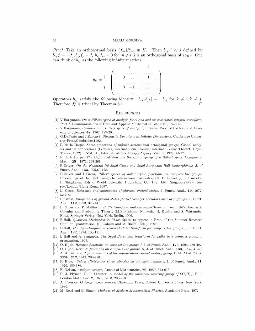
Proof. Take an orthonormal basis fm∞m=1 in Hr. Then bij , i < j defined bybijfi = −fj , bijfj = fi, bijfm = 0 for m 6= i, j is an orthogonal basis of soHS . Onecan think of bij as the following infinite matrices:
bij =
i j
i
j
. . . . . . . . . . . . . . . . . . . . . . . .
. . . 0 . . . . . . 1 . . .
. . . . . . . . . . . . . . . . . . . . . . . .
. . . 0 −1 . . . . . . . . . . .
. . . . . . . . . . . . . . . . . . . . . . . .
Operators bij satisfy the following identity: [bik, bjk] = −bij for k 6= i, k 6= j.Therefore J0
t is trivial by Theorem 8.1.
References
[1] V.Bargmann, On a Hilbert space of analytic functions and an associated integral transform,Part I, Communications of Pure and Applied Mathematics, 24, 1961, 187-214.
[2] V.Bargmann, Remarks on a Hilbert space of analytic functions, Proc. of the National Acad-emy of Sciences, 48, 1962, 199-204.
[3] G.DaPrato and J.Zabczyk, Stochastic Equations in Infinite Dimensions, Cambridge Univer-sity Press,Cambridge,1992.
[4] P. de la Harpe, Some properties of infinite-dimensional orthogonal groups, Global analy-sis and its applications (Lectures, Internat. Sem. Course, Internat. Centre Theoret. Phys.,Trieste, 1972) , Vol. II , Internat. Atomic Energy Agency, Vienna, 1974, 71-77.
[5] P. de la Harpe, The Clifford algebra and the spinor group of a Hilbert space, CompositioMath. 25 , 1972, 245-261.
[6] B.Driver, On the Kakutani-Ito-Segal-Gross and Segal-Bargmann-Hall isomorphisms, J. ofFunct. Anal., 133,1995,69-128.
[7] B.Driver and L.Gross, Hilbert spaces of holomorphic functions on complex Lie groups,Proceedings of the 1994 Taniguchi International Workshop (K. D. Elworthy, S. Kusuoka,I. Shigekawa, Eds.), World Scientific Publishing Co. Pte. Ltd, Singapore/New Jer-sey/London/Hong Kong, 1997.
[8] L. Gross, Existence and uniqueness of physical ground states, J. Funct. Anal., 10, 1972,52-109.
[9] L. Gross, Uniqueness of ground states for Schrodinger operators over loop groups, J. Funct.Anal., 112, 1993, 373-441.
[10] L. Gross and P. Malliavin, Hall’s transform and the Segal-Bargmann map, Ito’s StochasticCalculus and Probability Theory, (M.Fukushima, N. Ikeda, H. Kunita and S. Watanabe,Eds.), Springer-Verlag, New York/Berlin, 1996.
[11] B.Hall, Quantum Mechanics in Phase Space, to appear in Proc. of the Summer ResearchConf. on Quantization, (L. Coburn and M. Rieffel, Eds.), 1997.
[12] B.Hall, The Segal-Bargmann ’coherent state’ transform for compact Lie groups, J. of Funct.Anal., 122, 1994, 103-151.
[13] B.Hall and A. Sengupta, The Segal-Bargmann transform for paths in a compact group, inpreparation, 1997.
[14] O. Hijab, Hermite functions on compact Lie groups I, J. of Funct. Anal., 125, 1994, 480-492.[15] O. Hijab, Hermite functions on compact Lie groups II, J. of Funct. Anal., 133, 1995, 41-49.[16] A. A. Kirillov, Representations of the infinite-dimensional unitary group, Dokl. Akad. Nauk.
SSSR, 212, 1973, 288-290.[17] P. Kree, Calcul d’integrales et de derivees en dimension infinite, J. of Funct. Anal., 31,
1979, 150-186.[18] E. Nelson, Analytic vectors, Annals of Mathematics, 70, 1959, 572-615.[19] R. J. Plymen, R. F. Streater, A model of the universal covering group of SO(H)2, Bull.
London Math. Soc. 7, 1975, no. 3, 283-288.[20] A. Pressley, G. Segal, Loop groups, Clarendon Press, Oxford University Press, New York,
1986.[21] M. Reed and B. Simon, Methods of Modern Mathematical Physics, Academic Press, 1972.
HOLOMORPHIC FUNCTIONS ON AN INFINITE DIMENSIONAL GROUP 27
[22] Derek W. Robinson, Elliptic operators and Lie Groups, Clarendon Press, 1991.[23] I. E. Segal, Tensor algebras over Hilbert spaces. II, Ann. of Math., 63, 1956, 160-175.[24] I. E. Segal, Mathematical characterization of the physical vacuum for a linear Bose-Einstein
field. (Foundations of the dynamics of infinite systems. III), Illinois J. Math., 6, 1962, 500-523.
[25] I. E. Segal, Mathematical problems of relativistic physics, Lectures in Applied Mathematics(proceedings of the Summer Seminar, Boulder, Colorado, 1960), Vol. II American Mathemat-ical Society, Providence, R.I.
[26] I. Shigekawa, Ito-Wiener expansions of holomorphic functions on the complex Wiener space,in Stochastic Analysis, (E. Mayer et al, Eds.), Academic Press, San Diego, 1991, 459-473.
[27] S. Stratila, D. Voiculescu, A survey on representations of the unitary group U(∞), Spectraltheory (Warsaw, 1977), Banach Center Publ., 8, PWN, Warsaw, 1982, 415-434.
[28] H.Sugita, Properties of holomorphic Wiener functions-skeleton, contraction, and local Taylorexpansion, Probab. Theory Related Fields, 100, 1994, 117–130.
[29] H.Sugita, Regular version of holomorphic Wiener function, J. Math. Kyoto Univ., 34, 1994,849–857.
Department of Mathematics, Cornell University, Ithaca, New York 14853E-mail address: [email protected]