Home Production as a Substitute for Market Consumption: Reactions of Time-Use to Shocks in Housing Wealth * Jim Been † Susann Rohwedder ‡ Michael Hurd § November 2014 Abstract Shocks to income and wealth decrease the households monetary budget available. As a consequence, households respond by decreasing consumption spending. Income shocks, such as unexpected unem- ployment and retirement, also increase the time-budget available in addition to decreasing the monetary budget available. Some research has suggested that the additional time available enables households to substitute home production for purchased goods and services, effectively increasing their well-being beyond what a measure of spending would indicate. We aim to expand on this research by using data on time-use with data on categories of spending. We use wealth shocks in house values induced by the Great Recession to infer the extent to which households adjusted home production in response to de- creasing market consumption possibilities. For people whose time-budget did not change and who were affected by the shock, we find that a 1% decrease in consumption that can be substituted for by home production increases the time spent in home production activities by about 0.6%. This implies that a part of the decreased market consumption possibilities can be replaced by home production to mitigate the consequences for well-being. * The work was supported by a grant from the Social Security Administration through the Michigan Retirement Research Center (Grant #RRC08098401 - 06). This paper was written while Jim was a Visiting Researcher at the RAND Center for the Study on Aging at RAND Corporation. This research visit has been sponsored by Leiden University Fund/ van Walsem (Grant #4414/3 - 9 - 13\V, vW ) and the Leiden University Department of Economics. We have benefited from discussions with Marco Angrisani, Italo Lopez-Garcia and Robert Willis. The findings and conclusions expressed are solely those of the authors and do not represent the opinions or policy of the Social Security Administration, any agency of the Federal government, or the Michigan Retirement Research Center. † Department of Economics at Leiden University and Netspar (e-mail address: [email protected]) ‡ RAND Corporation, Santa Monica, CA, USA, MEA and Netspar (e-mail address: [email protected]) § RAND Corporation, Santa Monica, CA, USA, NBER, MEA and Netspar (e-mail address: [email protected])
Transcript
Home Production as a Substitute for Market Consumption:
Reactions of Time-Use to Shocks in Housing Wealth ∗
Jim Been † Susann Rohwedder ‡ Michael Hurd §
November 2014
Abstract
Shocks to income and wealth decrease the households monetary budget available. As a consequence,
households respond by decreasing consumption spending. Income shocks, such as unexpected unem-
ployment and retirement, also increase the time-budget available in addition to decreasing the monetary
budget available. Some research has suggested that the additional time available enables households
to substitute home production for purchased goods and services, effectively increasing their well-being
beyond what a measure of spending would indicate. We aim to expand on this research by using data
on time-use with data on categories of spending. We use wealth shocks in house values induced by the
Great Recession to infer the extent to which households adjusted home production in response to de-
creasing market consumption possibilities. For people whose time-budget did not change and who were
affected by the shock, we find that a 1% decrease in consumption that can be substituted for by home
production increases the time spent in home production activities by about 0.6%. This implies that a
part of the decreased market consumption possibilities can be replaced by home production to mitigate
the consequences for well-being.
∗The work was supported by a grant from the Social Security Administration through the Michigan Retirement Research
Center (Grant #RRC08098401− 06). This paper was written while Jim was a Visiting Researcher at the RAND Center for
the Study on Aging at RAND Corporation. This research visit has been sponsored by Leiden University Fund/ van Walsem
(Grant #4414/3− 9− 13\V,vW ) and the Leiden University Department of Economics. We have benefited from discussions
with Marco Angrisani, Italo Lopez-Garcia and Robert Willis. The findings and conclusions expressed are solely those of
the authors and do not represent the opinions or policy of the Social Security Administration, any agency of the Federal
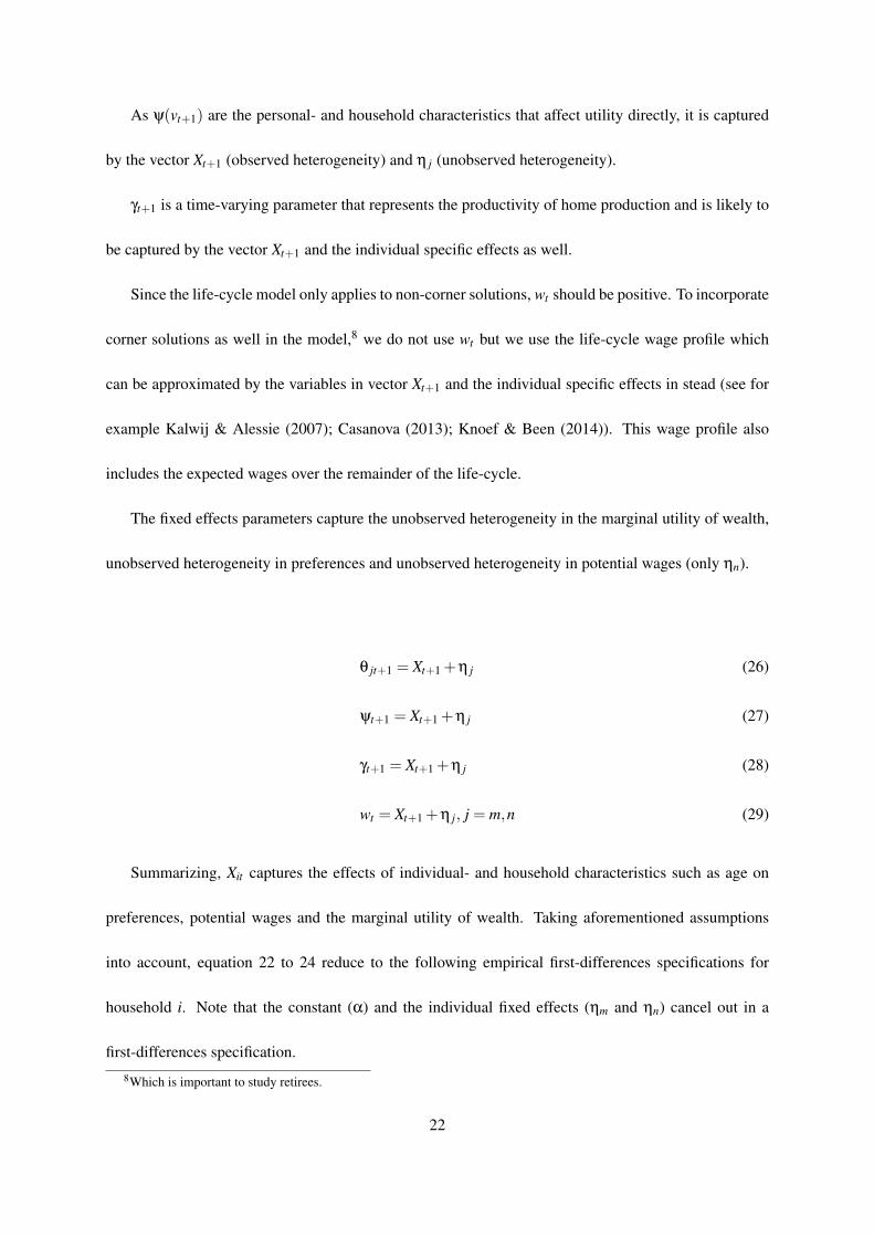
government, or the Michigan Retirement Research Center.†Department of Economics at Leiden University and Netspar (e-mail address: [email protected])‡RAND Corporation, Santa Monica, CA, USA, MEA and Netspar (e-mail address: [email protected])§RAND Corporation, Santa Monica, CA, USA, NBER, MEA and Netspar (e-mail address: [email protected])
JEL codes:
Keywords: Home production, Time-use, Consumption, Well-being, Wealth shocks, Great Recession
2
1 Introduction
The assessment of economic preparation for retirement has relied on measures of income and wealth
(Boskin & Shoven, 1987; Haveman et al., 2006, 2007; Crawford & O’Dea, 2012; Knoef et al., 2013;
De Bresser & Knoef, 2014), and in some cases on measures of consumption (Engen et al., 1999; Scholz
et al., 2006; Hurd & Rohwedder, 2008, 2011; Binswanger & Schunk, 2012). The canonical Life-Cycle
Hypothesis (LCH) predicts that individuals allocate their resources in order to smooth the marginal util-
ity of consumption over their life-time. To obtain smoothing of consumption over life-time, rational
forward-looking individuals will save during the working life so to maintain a smooth level of consump-
tion at retirement by dissaving. Using a life-cycle model Scholz et al. (2006) find that about 80% of
Americans are saving sufficiently to smooth their marginal utility of consumption over the life-cycle.
Hurd & Rohwedder (2011) find a similar result of the adequacy of preparation for retirement.
While none of these studies consider home production in their assessments, a couple of strands
of related literature have raised the issue and showed that home production plays a role when people
experience a change in their work status. The first literature is concerned with changes in spending
and time use around retirement and the second is concerned with changes in spending and time use
in response to unemployment. A number of studies have noted and investigated a sizeable drop in
household spending at retirement. This phenomenon of sharply declining consumption at retirement has
been called the retirement consumption puzzle as it is in contrast with the predictions of the LCH. Such
drops in consumption expenditures at retirement are found by, among others, Mariger (1987); Robb
& Burbidge (1989); Banks et al. (1998); Bernheim et al. (2001); Miniaci et al. (2003); Battistin et al.
(2009). Other studies argue that the drop in consumption expenditures at retirement is not in contrast
with the LCH. Hurd & Rohwedder (2003, 2006); Ameriks et al. (2007); Borella et al. (2011); Hurd
3
& Rohwedder (2013) argue that the drop in consumption is anticipated and therefore not inconsistent
with rational forward-looking individuals per se. On the other hand, retirement may be an unanticipated
shock (due to a health shock or layoffs) as suggested by Smith (2006); Haider & Stephens (2007);
Barrett & Brzozowski (2012). Such unexpected retirement may explain the drop in consumption that is
empirically observed while being consistent with the LCH. For an excellent overview of the literature
regarding the reconciliation of consumption drops within the LCM, see Hurst (2008) and Attanasio &
Weber (2010).
One of the main conclusions of Hurst (2008) is that a large heterogeneity is found in spending
changes at retirement across different categories of consumption. Especially food expenditures are found
to fall sharply relative to other consumption components at retirement (Aguila et al., 2011; Hurd &
Rohwedder, 2013; Velarde & Herrmann, 2014). Aguiar & Hurst (2005) explain this phenomenon by
showing that retired persons use their additionally available time to maintain well-being by substituting
home production (e.g., cooking) for purchased goods and services (e.g., dining out). Stancanelli &
Van Soest (2012) show that the act of retirement increases time spent in home production. Hence, it is
crucial to differentiate between expenditures and consumption and to augment the standard life-cycle
model with home production in order to explain that the expenditure drops observed at retirement are
not inconsistent with the LCH (Hurst, 2008).
The idea of introducing home produced good in the utility function was introduced by Becker (1965)
and further developed by Gronau (1977). In dynamic equilibrium, an individual maximizes within period
utility by equating marginal utilities to price ratios, where the price of time depends on labor market
opportunities. Following retirement as total spending declines, budget shares will change as predicted
by Engle curves; to the extent that some uses of time are complements or substitutes for each type of
4
purchased consumption good, those uses of time will also change.
The subsequent literature has pursued the implications of home production further. Baxter & Jer-
mann (1999); Apps & Rees (2005); Aguiar & Hurst (2005); Dotsey et al. (2010); Rogerson & Wallenius
(2013) incorporate home production in a standard life-cycle model in which the home produced goods
are substitutable with market goods. Dotsey et al. (2010) show that this model can account for the ob-
served patterns in consumption and time-use over the life-cycle. According to the model, households
allocate more time to home production and leisure as they reduce working hours toward retirement. This
is because the opportunity cost of home production and leisure declines in retirement, because there is
no longer a tradeoff with working hours. As a consequence, home production of goods substitutes for
consumption of market goods; this explains the drop in expenditures observed at retirement.
Taking into account the willingness to substitute home production for market consumption also
improves explanation of the aggregate fluctuations observed at the macro level (Benhabib et al., 1991;
Greenwood & Hercowitz, 1991). The time households devote to home production fluctuates over the
business cycle, implying that households may shift away from market work to home production in
recessional times. Unemployed workers choose lower levels of market goods consumption than they
would if employed, but they can keep well-being constant as they have more time to produce at home
(Hall, 2009; Karabarbounis, 2014). Ahn et al. (2008) find that home production is higher in households
with unemployed individuals than in those with employed individuals. Similarly, Brzozowski & Lu
(2006), explicitly focusing on food consumption and production, find that home production is higher in
households with retired individuals.
Although these results are an indication of substitution effects between market consumption and
time-use, they cannot be interpreted as being causal; Ahn et al. (2008) and Brzozowski & Lu (2006)
5
are only able to analyze time-use in a cross-sectional setting. However, using longitudinal data, Velarde
& Herrmann (2014) find substantial substitution effects between food expenditures and food-related
time-use at retirement. This result extends to individuals who are non-working (not in the labor force) or
unemployed. Such effects are also found by Colella & Van Soest (2013) focusing on home production in
general. Burda & Hamermesh (2010) find evidence that individuals generally offset market hours with
home production during times of high cyclical unemployment. Aguiar et al. (2013) show that individuals
who lost working hours during the Great Recession reallocated a substantial part of their available time
to home production and/or increased leisure time. They find that about 30% of lost working hours
were absorbed by home production during the Great Recession. Such substitution between market work
and home production may mitigate the effects of recessions on well-being, the drop in which may not
be as large as the drop in market hours. However, Aguiar et al. (2013) do not study the substitution
effects between market consumption and home production as they do not have data on spending (Burda
& Hamermesh, 2010; Aguiar et al., 2013). Analyzing the effect of the Great Recession, Griffith et al.
(2014) find that households lowered food spending by increased shopping effort. They, however, do not
have any explicit information about time-use.
We expand on the research discussed above by using data that has information on both time-use and
spending such as Colella & Van Soest (2013); Velarde & Herrmann (2014). Compared to Colella &
Van Soest (2013); Velarde & Herrmann (2014) we explicitly try to find the degree of substitution be-
tween consumption spending and home production. Since spending on market consumption and home
production is endogenous, we use the wealth shocks induced by the Great Recession to infer the degree
to which households are able to use time to offset partially the market consumption possibilities losses.
More particularly, we use the the drop in house prices as an exogenous negative wealth shock that de-
6
creased the monetary budget (Angrisani et al., 2013) but not the time budget. Angrisani et al. (2013)
exploit regional heterogeneity in house price drops due to the Great Recession to infer a causal relation-
ship between wealth and consumption. They find substantial decreases in consumption due to the drop
in housing wealth due to the Great Recession. Substitution effects between consumption spending and
time-use is, however, neglected in this study. Nevertheless, it is important to gain insight into the degree
to which consumption can be replaced by home production as this may mitigate the effects of shocks on
well-being.
The remainder of the paper is organized as follows. Section 2 describes the HRS and CAMS data
used in the paper. Descriptive statistics of time-use and consumption spending are presented in Sec-
tion 3. To analyze home production formally, Section 4 presents a simple life-cycle model with home
production. The functional form and the empirical model are dervied in Section 5 and Section 6 re-
spectively. The results of the empirical model are shown in Section 7. Section 8 provides a discussion.
Conclusions regarding the substitutability of market consumption and home production can be found in
Section 9.
2 Data
The data for our empirical analyses come from the Health and Retirement Study (HRS), a longitudi-
nal survey that is representative of the U.S. population over the age of 50 and their spouses. The HRS
conducts core interviews of about 20,000 persons every two years. In addition the HRS conducts supple-
mentary studies to cover specific topics beyond those covered in the core surveys. The time-use data we
use in this paper were collected as part of such a supplementary study, the Consumption and Activities
Mail Survey (CAMS).
7
Health and Retirement Study Core interviews
The first wave of the HRS was fielded in 1992. It interviewed people born between 1931 and 1941 and
their spouses, irrespective of age. The HRS re-interviews respondents every second year. Additional
cohorts have been added so that beginning with the 1998-wave the HRS is representative of the entire
population over the age of 50. The HRS collects detailed information on the health, labor force participa-
tion, economic circumstances, and social well-being of respondents. The survey dedicates considerable
time to elicit income and wealth information, providing a complete inventory of the financial situation
of households. In this study we use demographic and asset and income data from the HRS core waves
spanning the years 2002 through 2010.
Consumption and Activities Mail Survey
The CAMS survey aims to obtain detailed measures of time-use and total annual household spending on
a subset of HRS respondents. These measures are merged to the data collected on the same households
in the HRS core interviews. The CAMS surveys are conducted in the HRS off-years, that is, in odd-
numbered years.
The first wave of CAMS was collected in 2001 and it has been collected every two years since. Ques-
tionnaires are sent out in late September or early October. Most questionnaires are returned in October
and November. CAMS thus obtains a snap-shot of time-use observed in the fall of the CAMS survey
year. In the first wave, 5,000 households were chosen at random from the entire pool of households who
participated in the HRS 2000 core interview. Only one person per household was chosen. About 3,800
HRS households responded, so CAMS 2001 was a survey of the time-use of 3,800 respondents and the
total household spending of the 3,800 households in which these respondents live. Starting in the third
wave of CAMS, both respondents in a couple household were asked to complete the time-use section,
8
so that the number of respondent-level observations on time use in each wave was larger for the waves
from 2005 and onwards.
Respondents were asked about a total of 31 time-use categories in wave 1; wave 2 added two more
categories; wave 4 added 4 additional categories. Thus, since CAMS 2007 the questionnaire elicits
37 time-use categories, as shown in Appendix A. Of particular interest for this study are the CAMS
time-use categories related to home production:
• House cleaning
• Washing, ironing or mending clothes
• Yard work or gardening
• Shopping or running errands
• Preparing meals and cleaning up afterwards
• Taking care of finances or investments, such as banking, paying bills, balancing the checkbook,
doing taxes, etc.
• Doing home improvements, including painting, redecorating, or making home repairs
• Working on, maintaining, or cleaning car(s) and vehicle(s)
For most activities respondents are asked how many hours they spent on this activity last week. For less
frequent categories they were asked how many hours they spent on these activities last month. Hurd &
Rohwedder (2008) provide a detailed overview of the time-use section of CAMS, its design features
and structure, and descriptive statistics. A detailed comparison of time-use as recorded in CAMS with
that recorded in the American Time Use Survey (ATUS) shows summary statistics that are fairly close
9
across the two surveys, despite a number of differences in design and methodology (Hurd & Rohwedder,
2007).
In this paper we use data from CAMS 2005, 2007, 2009 and 2011, each wave containing between
about 5,300 and 6,500 respondent-level observations on time-use that we merge with HRS core data.
Combining the data from the HRS core and the CAMS provides us with data that are unique in that
we observe demographics, economic status, time-use and spending for the same individuals and their
households in panel.
3 Descriptive statistics
3.1 Time-use
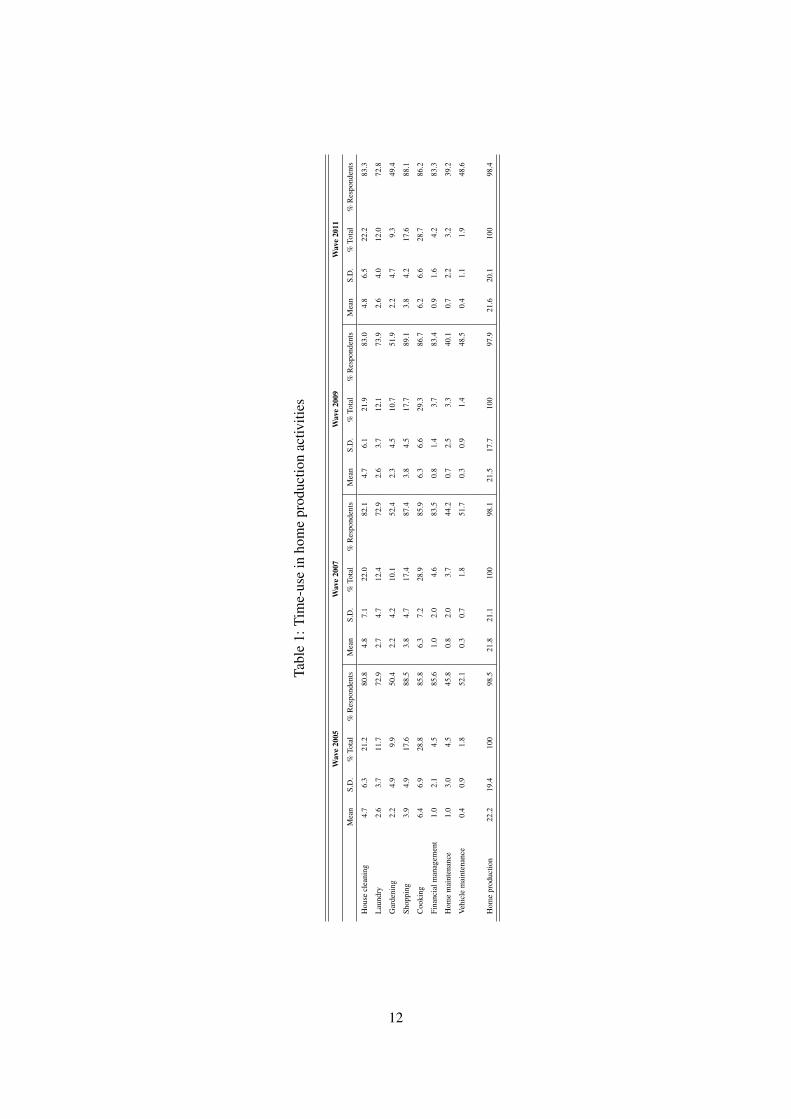
Table 1 shows the time spent in home production activities per wave by persons aged 51-80. These
activities can be used as a substitute for the market bought goods and services shown in Table 2. The
aggregate of home production activities shows that a non-negligible part of the weekly available time is
spent on home production and that virtually all persons engage in some form of home production.
Most of the home production is devoted to the cooking of meals. Together with the house cleaning,
this accounts for about half of total time spent in home production. More than 80% of the persons in
the data spend some time on these two home production activities. About 90% of the people engage in
shopping activities although the average time spent in this activity is somewhat smaller than the time
spent in house cleaning and cooking. Unlike activities such as house cleaning, cooking and doing the
laundry, it is harder to buy the service for shopping on the market which may explain the relatively high
percentage of persons engaging in this activity. Approximately half of the people engage in gardening
and maintenance of the home and vehicles but the amount of time spent in these activities are fairly
10
small. More than 80% of the people spend time on managing their finances, but the amount of time
spent in this activity is only about an hour per week.
Despite the fact that a non-negligible part of the weekly available time is devoted to home production
activities on average, there is a lot of variation around this average as the standard deviations of most
activities are about the same size as the averages (or even bigger). However, the variation across waves
is only marginal. This might suggest that people do not adjust their time-use in home production that
much during the course of the business cycle.
3.2 Consumption
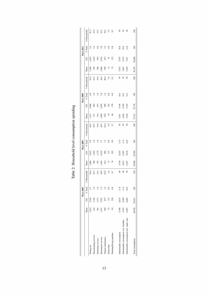
Table 2 shows the household spending on consumption that can be substituted for by home production.
The waves prior to the Great Recession show that spending is on average more substantial than in the
waves after the Great Recession. This is consistent with the consumption drops found by Angrisani et
al. (2013).
Substitutable consumption is about 11-12% of total consumption spending and is consistent across
waves. This makes the substitutable consumption spending a non-negligible part of total consumption
spending. The biggest component of the substitutable consumption spending consists of dining out ex-
penditures. This expenditure could be well substituted for by home production in the form of cooking.
Standard deviations of the spending categories are relatively big compared to the mean. The relative size
of the standard deviation compared to the mean is much smaller for the total of consumption spending.
This suggest that there is especially large heterogeneity in consumption spending that could be substi-
tuted for by home production activities. We observe that virtually all households have expenditures that
could be substituted for by home production although the percentage of households with spending on
substitutable consumption decreased in later waves.
11
Tabl
e1:
Tim
e-us
ein
hom
epr
oduc
tion
activ
ities
Wav
e20
05W
ave
2007
Wav
e20
09W
ave
2011
Mea
nS.
D.
%To
tal
%R
espo
nden
tsM
ean
S.D
.%
Tota
l%
Res
pond
ents
Mea
nS.
D.
%To
tal
%R
espo
nden
tsM
ean
S.D
.%
Tota
l%
Res
pond
ents
Hou
secl
eani
ng4.
76.
321
.280
.84.
87.
122
.082
.14.
76.
121
.983
.04.
86.
522
.283
.3
Lau
ndry
2.6
3.7
11.7
72.9
2.7
4.7
12.4
72.9
2.6
3.7
12.1
73.9
2.6
4.0
12.0
72.8
Gar
deni
ng2.
24.
99.
950
.42.
24.
210
.152
.42.
34.
510
.751
.92.
24.
79.
349
.4
Shop
ping
3.9
4.9
17.6
88.5
3.8
4.7
17.4
87.4
3.8
4.5
17.7
89.1
3.8
4.2
17.6
88.1
Coo
king
6.4
6.9
28.8
85.8
6.3
7.2
28.9
85.9
6.3
6.6
29.3
86.7
6.2
6.6
28.7
86.2
Fina
ncia
lman
agem
ent
1.0
2.1
4.5
85.6
1.0
2.0
4.6
83.5
0.8
1.4
3.7
83.4
0.9
1.6
4.2
83.3
Hom
em
aint
enan
ce1.
03.
04.
545
.80.
82.
03.
744
.20.
72.
53.
340
.10.
72.
23.
239
.2
Veh
icle
mai
nten
ance
0.4
0.9
1.8
52.1
0.3
0.7
1.8
51.7
0.3
0.9
1.4
48.5
0.4
1.1
1.9
48.6
Hom
epr
oduc
tion
22.2
19.4
100
98.5
21.8
21.1
100
98.1
21.5
17.7
100
97.9
21.6
20.1
100
98.4
12
Tabl
e2:
Hou
seho
ldle
velc
onsu
mpt
ion
spen
ding
Wav
e20
05W
ave
2007
Wav
e20
09W
ave
2011
Mea
nS.
D.
%To
tal
%H
ouse
hold
sM
ean
S.D
.%
Tota
l%
Hou
seho
lds
Mea
nS.
D.
%To
tal
%H
ouse
hold
sM
ean
S.D
.%
Tota
l%
Hou
seho
lds
Din
ing
out
1,91
23,
530
4.7
85.0
1,80
82,
912
4.5
84.5
1,51
32,
096
4.0
83.9
1,59
82,
443
4.4
81.2
Hou
seke
epin
gse
rvic
es41
41,
194
1.0
49.3
386
1,05
41.
049
.533
198
41.
045
.234
91,
014
1.0
43.4
Gar
deni
ngse
rvic
es38
11,
371
1.0
34.2
355
1,17
91.
033
.831
483
31.
035
.629
685
40.
833
.5
Hom
erep
airs
ervi
ces
1,34
73,
923
3.3
49.8
1,46
56,
515
3.7
48.5
1,06
82,
829
2.8
48.4
1,00
63,
534
2.8
43.2
Veh
icle
mai
nten
ance
649
875
1.6
83.0
614
804
1.5
81.6
618
809
1.6
80.4
598
833
1.6
78.2
Dis
hwas
her
2311
50.
04.
427
127
0.0
5.0
1910
50.
03.
615
910.
03.
5
Was
hing
/Dry
ing
mac
hine
6325
00.
08.
776
293
0.0
9.7
6827
80.
09.
253
232
0.0
8.3
Subs
titut
able
cons
umpt
ion
4,78
86,
633
11.8
964,
730
8,25
311
.995
3,93
14,
748
10.5
953,
915
5,55
710
.894
Subs
titut
able
cons
umpt
ion
excl
.dur
able
s4,
703
6,59
011
.696
4,62
78,
201
11.6
953,
844
4,70
010
.295
3,84
75,
515
10.6
93
Subs
titut
able
cons
umpt
ion
incl
.sup
pl.m
at.
6,48
78,
069
16.0
996,
387
9,87
816
.099
5,34
25,
795
14.2
995,
382
7,07
114
.898
Tota
lcon
sum
ptio
n40
,558
29,4
2710
010
039
,904
29,2
6810
010
037
,515
25,7
7810
010
036
,359
26,0
8610
010
0
13
Together, Table 1 and Table 2 give some idea on the scope of substituting market purchases for
home production activities. To capture the possible substitution effects between the two more formally,
we present a life-cycle model with home production in the next section.
4 Model
4.1 A simple Life-Cycle Model
The standard model to analyze consumption over the life-cycle is the life-cycle model that expresses
utility over the remainder of the life-cycle as a function of consumption and leisure. Households maxi-
mize
Uτ = maxEτ
[T
∑t=τ
(1+ρ)τ−tu(ct , lt)ψ(vt)
](1)
where ct and lt denote consumption and leisure in time period t, respectively. ρ is the discount factor and
T the time horizon of the household. vt are the personal- and household characteristics that influence
utility directly known as taste-shifters (e.g. age, household size, number of children).
Households maximize Equation 1 under the budget constraint that
At+1 = (1+ r)(At +(wt · (H− lt))+bt − ct) (2)
where At is the amount of assets at time t, r is a constant real interest rate, wt is the (after-tax) wage
rate, H the time-endowment and bt are benefits (e.g. unemployment, social security and other unearned
non-asset income).
An extension introduces leisure interacting with the one good in the instantaneous utility function
so as to allow for home production, and/or complementarity or substitutability between time and that
14
good (Laitner & Silverman, 2005). However, following retirement leisure is fixed so that this version of
the extended model reverts to the simple version. Therefore home-production needs to be incorporated
explicitly in the life-cycle model.
4.2 A simple Life-Cycle Model with Home Production
Since we are particularly interested in time-use, it is important to incorporate household production
(Becker, 1965; Gronau, 1977; Apps & Rees, 1997, 2005) in the simple life-cycle model . This introduces
home produced goods cnt next to the classical market consumption cmt and leisure lt (Rupert et al., 2000)
which yields the following utility function
Uτ = maxEτ
[T
∑t=τ
(1+ρ)τ−tu(cmt ,cnt(hnt), lt)ψ(vt)
](3)
with cnt(hnt) = gt(hnt) being the home production function with time spent in home production hnt .
For simplicity, we assume that the home production function is strictly concave in one variable input,1
namely the time spent in home production. The budget constraint becomes
where ξt yields a random term that captures a shock in the value of wealth available at time t (At). We
assume Et [ξt ] = 0 in the marginal utility of wealth. A shock at time t ([ξt ] 6= 0) is captured by the error
term εt+1 in Equations 8-10.
17
A negative shock (ξt < 0) causes the monetary budget available at time t+1 (At+1) to decrease. This
means that the decreased monetary budget has consequences for hmt+1, hnt+1, lt+1, cmt+1 and cnt+1 in
reoptimizing utility from the remaining life-time. As a result of the wealth shock, individuals may react
by 1) only reducing market consumption (cmt), 2) only increasing market work (hmt) at the expense of
leisure (lt), 3) switching from market consumption (cmt) to non-market consumption (cnt) (e.g. home
production) or a combination of these options.
Option 1) is most likely to have the most substantial effects on well-being while option 2) may not
be possible (e.g. people working full-time, hours constraints by employers, retirees, unemployment,
disability,). This suggests that option 3) would be a favorable option to mitigate the consequences of
a negative wealth shock on well-being. Especially for those individuals that are unable to adjust their
market hours (hmt). The shift from market produced to home produced consumption goods would imply
an increase in the total time spent in home production activities (hnt).
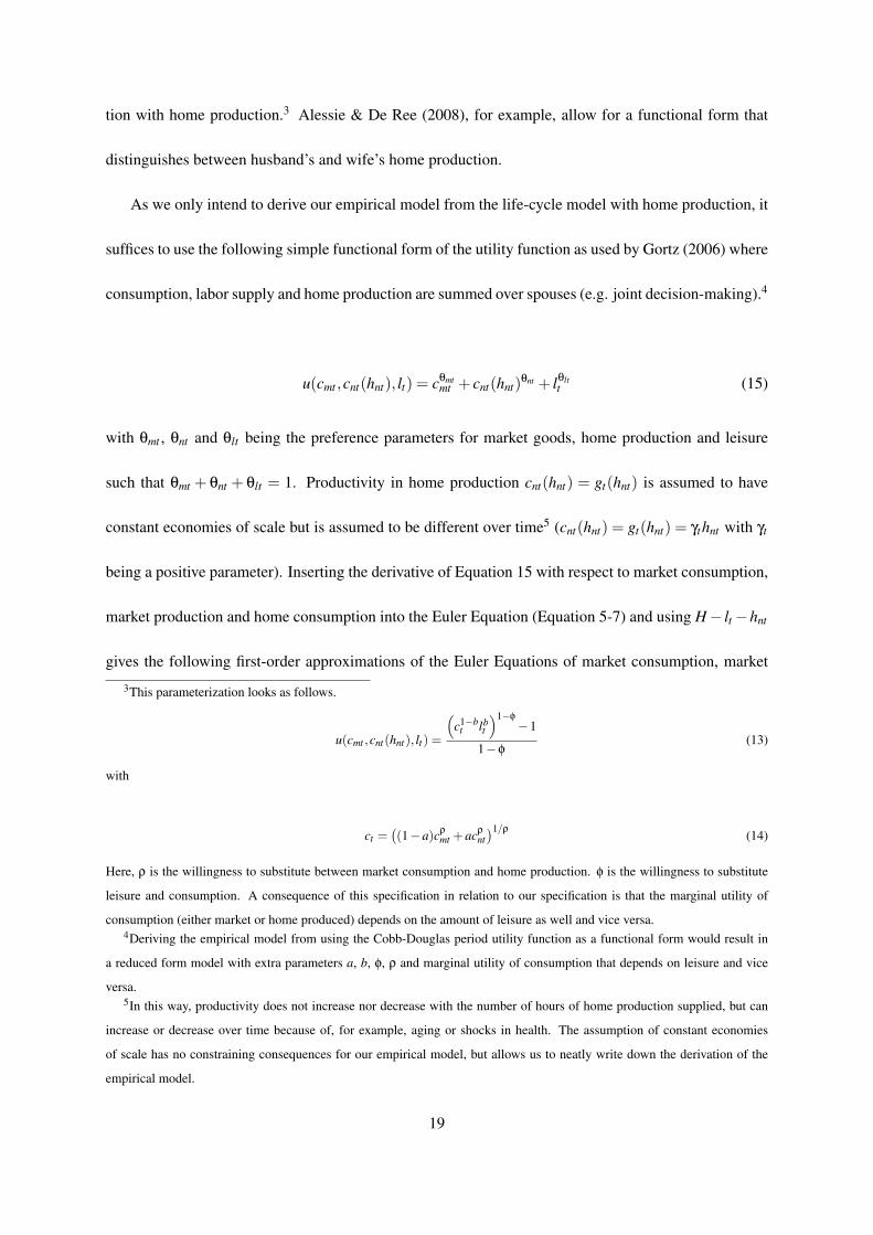
5 A functional form to derive the empirical model
For simplicity, the functional form representation of preferences for market consumption, home con-
sumption and labor is an additive utility function such that preferences are additively separable.2 A
similar simple functional form of the utility function was used by Rupert et al. (2000) and Gortz (2006).
More sophisticated functional forms are used in Benhabib et al. (1991), Greenwood & Hercowitz (1991),
Fang & Zhu (2012), Dotsey et al. (2010), Rogerson & Wallenius (2013) and Karabarbounis (2014).
These papers use a Cobb-Douglas period utility function as a CES parameterization of the utility func-
2We assume additively separable preferences in this framework to keep the derivation of our empirical model tractable. In
practice, it is likely that the marginal utility of consumption does depend on home production, for example.
18
tion with home production.3 Alessie & De Ree (2008), for example, allow for a functional form that
distinguishes between husband’s and wife’s home production.
As we only intend to derive our empirical model from the life-cycle model with home production, it
suffices to use the following simple functional form of the utility function as used by Gortz (2006) where
consumption, labor supply and home production are summed over spouses (e.g. joint decision-making).4
u(cmt ,cnt(hnt), lt) = cθmtmt + cnt(hnt)
θnt + lθltt (15)
with θmt , θnt and θlt being the preference parameters for market goods, home production and leisure
such that θmt + θnt + θlt = 1. Productivity in home production cnt(hnt) = gt(hnt) is assumed to have
constant economies of scale but is assumed to be different over time5 (cnt(hnt) = gt(hnt) = γthnt with γt
being a positive parameter). Inserting the derivative of Equation 15 with respect to market consumption,
market production and home consumption into the Euler Equation (Equation 5-7) and using H− lt−hnt
gives the following first-order approximations of the Euler Equations of market consumption, market
3This parameterization looks as follows.
u(cmt ,cnt(hnt), lt) =
(c1−b
t lbt
)1−φ
−1
1−φ(13)
with
ct =((1−a)cρ
mt +acρ
nt)1/ρ
(14)
Here, ρ is the willingness to substitute between market consumption and home production. φ is the willingness to substitute
leisure and consumption. A consequence of this specification in relation to our specification is that the marginal utility of
consumption (either market or home produced) depends on the amount of leisure as well and vice versa.4Deriving the empirical model from using the Cobb-Douglas period utility function as a functional form would result in
a reduced form model with extra parameters a, b, φ, ρ and marginal utility of consumption that depends on leisure and vice
versa.5In this way, productivity does not increase nor decrease with the number of hours of home production supplied, but can
increase or decrease over time because of, for example, aging or shocks in health. The assumption of constant economies
of scale has no constraining consequences for our empirical model, but allows us to neatly write down the derivation of the
empirical model.
19
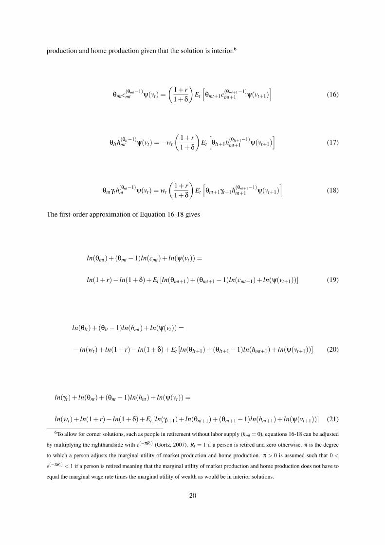
production and home production given that the solution is interior.6
θmtc(θmt−1)mt ψ(vt) =
(1+ r1+δ
)Et
[θmt+1c(θmt+1−1)
mt+1 ψ(vt+1)]
(16)
θlth(θlt−1)mt ψ(vt) =−wt
(1+ r1+δ
)Et
[θlt+1h(θlt+1−1)
mt+1 ψ(vt+1)]
(17)
θntγth(θnt−1)nt ψ(vt) = wt
(1+ r1+δ
)Et
[θnt+1γt+1h(θnt+1−1)
nt+1 ψ(vt+1)]
(18)
The first-order approximation of Equation 16-18 gives
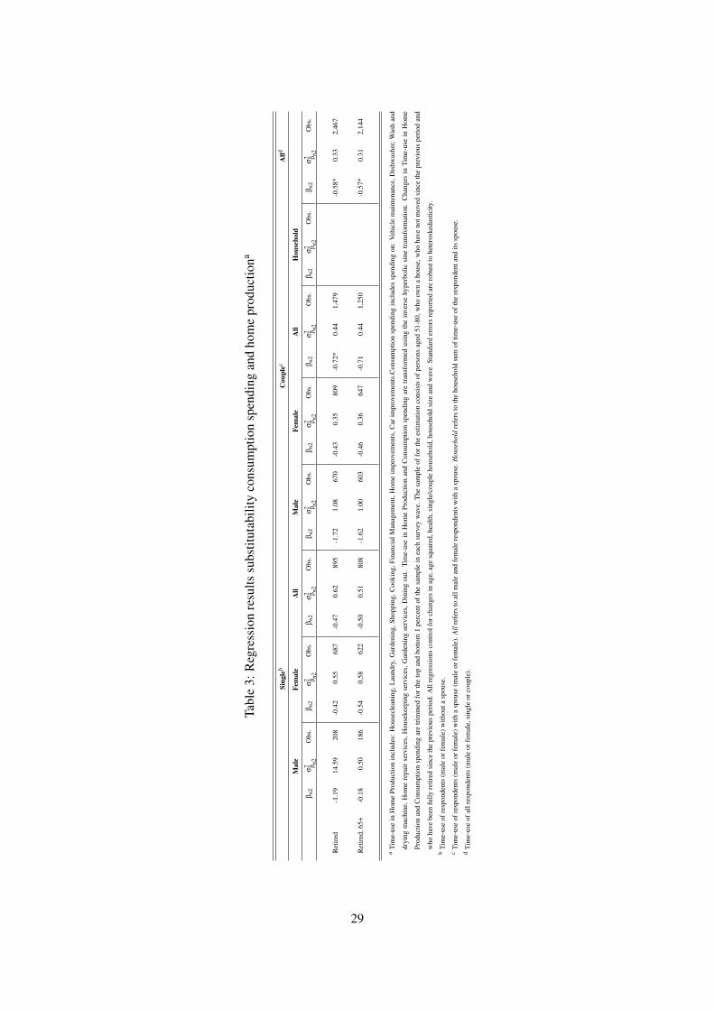
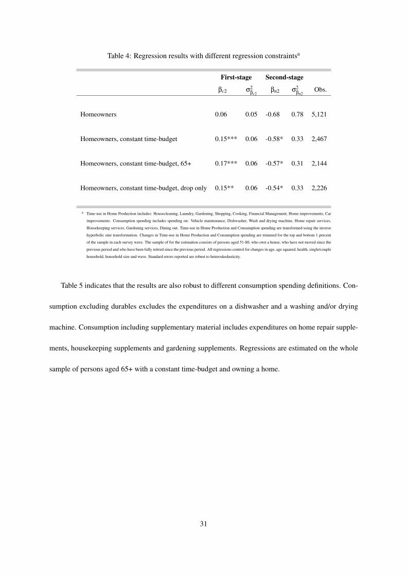
Homeowners, constant time-budget, drop only 0.15** 0.06 -0.54* 0.33 2,226
a Time-use in Home Production includes: Housecleaning, Laundry, Gardening, Shopping, Cooking, Financial Management, Home improvements, Car
improvements. Consumption spending includes spending on: Vehicle maintenance, Dishwasher, Wash and drying machine, Home repair services,
Housekeeping services, Gardening services, Dining out. Time-use in Home Production and Consumption spending are transformed using the inverse
hyperbolic sine transformation. Changes in Time-use in Home Production and Consumption spending are trimmed for the top and bottom 1 percent
of the sample in each survey wave. The sample of for the estimation consists of persons aged 51-80, who own a house, who have not moved since the
previous period and who have been fully retired since the previous period. All regressions control for changes in age, age squared, health, single/couple
household, household size and wave. Standard errors reported are robust to heteroskedasticity.
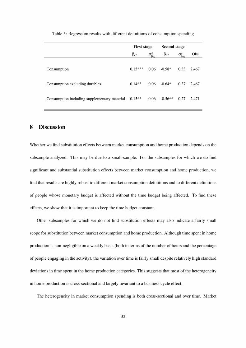
Table 5 indicates that the results are also robust to different consumption spending definitions. Con-
sumption excluding durables excludes the expenditures on a dishwasher and a washing and/or drying
machine. Consumption including supplementary material includes expenditures on home repair supple-
ments, housekeeping supplements and gardening supplements. Regressions are estimated on the whole
sample of persons aged 65+ with a constant time-budget and owning a home.
31
Table 5: Regression results with different definitions of consumption spending