Homework 2 solutions

Problem 1 (10.1)a) Starting from the LHS of the equation, note that

The first and third terms in the expression above are equal, differing only by a choice in indexing

notation between and . Hence the expression above is equal to:

b) The result of part (a) is that objective (10.11) is equivalent to the objective:

That is, minimize the sum of distances from observations to their centroids. Note that in Algorithm

10.1, with each iteration there are two steps: (a) compute each cluster centroid and (b) assign each

observation to the nearest centroid. Step (a) necessarily decreases this objective because the cluster

centroid is the point which minimizes the sum of squared distances to its members, and step (b)

necessarily decreases this objective because assigning each observation to the nearest centroid

minimizes the distance from it to the centroid.

Problem 2 (10.2)

dissimilarity = as.dist(matrix(c(0, 0.3, 0.4, 0.7, 0.3, 0, 0.5, 0.8, 0.4, 0.5, 0, 0.45, 0.7, 0.8, 0.45, 0), 4, 4))

a. Complete linkage:

plot(hclust(dissimilarity), axes = F, xlab = NA)axis(2, at = c(0.3, 0.45, 0.8))

b. Single linkage:

plot(hclust(dissimilarity, method = "single"), axes = F, xlab = NA)axis(2, at = c(0.3, 0.4, 0.45))

c. The two clusters would be {1,2} and {3,4}.

d. The two clusters would be {1,2,3} and {4}.

e. Below is one possible solution to this problem, but answers may vary greatly.

plot(hclust(dissimilarity), labels = c("2", "1", "4", "3"), axes = F, xlab = NA)axis(2, at = c(0.3, 0.45, 0.8))

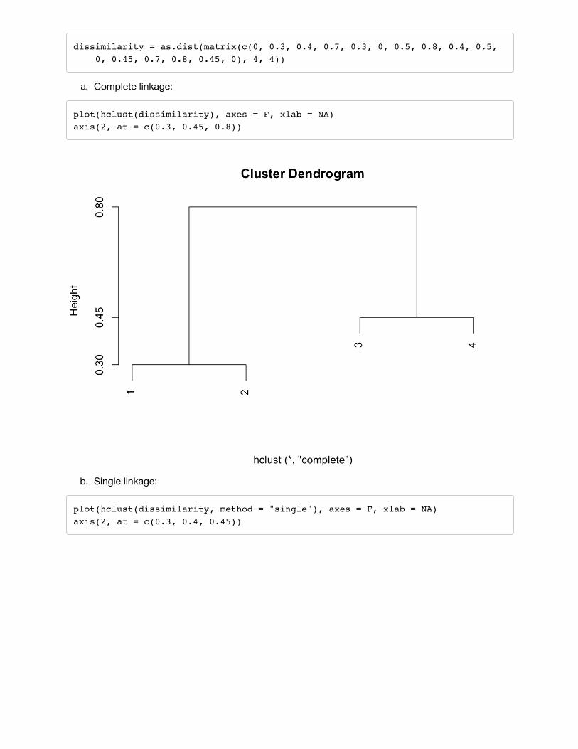
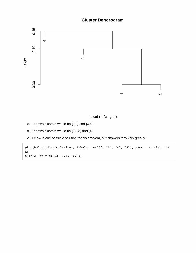
Problem 3 (10.4)a) The fusion will occur higher on the complete linkage dendrogram at height

where is the dissimilarity between and . The fusion on the single linkage dendrogram willoccur at the lower height

Note that in very special circumstances, the two heights could be equal.

b) Both fusions would occur at the same height on their respective trees, at height equal to thedissimilarity between 5 and 6.

Problem 4 (10.9)a. Clustering before scaling variables:

plot(hclust(dist(USArrests)), xlab = "State")

Text

3

b. The three clusters are: {FL,NC,DE,AL,LA,AK,MS,SC,MD,AZ,NM,CA,IL,NY,MI,NV}{MO,AR,TN,GA,CO,TX,RI,WY,OR,OK,VA,WA,MA,NJ}{OH,UT,CT,PA,NE,KY,MT,ID,IN,KS,HI,MN,WI,IA,NH,WV,ME,SD,ND,VT}

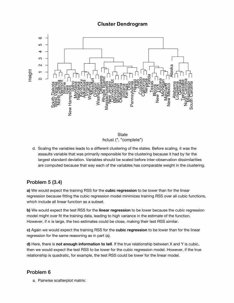
c. Clustering after scaling variables:

plot(hclust(dist(scale(USArrests, center = T))), xlab = "State")

d. Scaling the variables leads to a different clustering of the states. Before scaling, it was the

assaults variable that was primarily responsible for the clustering because it had by far the

largest standard deviation. Variables should be scaled before inter-observation dissimilarities

are computed because that way each of the variables has comparable weight in the clustering.

Problem 5 (3.4)a) We would expect the training RSS for the cubic regression to be lower than for the linear

regression because fitting the cubic regression model minimizes training RSS over all cubic functions,

which include all linear function as a subset.

b) We would expect the test RSS for the linear regression to be lower because the cubic regression

model might over fit the training data, leading to high variance in the estimate of the function.

However, if is large, the two estimates could be close, making their test RSS similar.

c) Again we would expect the training RSS for the cubic regression to be lower than for the linear

regression for the same reasoning as in part (a).

d) Here, there is not enough information to tell. If the true relationship between X and Y is cubic,

then we would expect the test RSS to be lower for the cubic regression model. However, if the true

relationship is quadratic, for example, the test RSS could be lower for the linear model.

Problem 6a. Pairwise scatterplot matrix:

library(ISLR)Auto = na.omit(Auto)pairs(Auto)

b. Correlation matrix:

round(cor(Auto[, -9]), digits = 3)

## mpg cylinders displacement horsepower weight acceleration## mpg 1.000 -0.778 -0.805 -0.778 -0.832 0.423## cylinders -0.778 1.000 0.951 0.843 0.898 -0.505## displacement -0.805 0.951 1.000 0.897 0.933 -0.544## horsepower -0.778 0.843 0.897 1.000 0.865 -0.689## weight -0.832 0.898 0.933 0.865 1.000 -0.417## acceleration 0.423 -0.505 -0.544 -0.689 -0.417 1.000## year 0.581 -0.346 -0.370 -0.416 -0.309 0.290## origin 0.565 -0.569 -0.615 -0.455 -0.585 0.213## year origin## mpg 0.581 0.565## cylinders -0.346 -0.569## displacement -0.370 -0.615## horsepower -0.416 -0.455## weight -0.309 -0.585## acceleration 0.290 0.213## year 1.000 0.182## origin 0.182 1.000

c. Note that the variable origin is categorical, but has been coded as a quantitative variable. Weshould correct this before moving on with the regression analysis:

Auto$origin = factor(Auto$origin)autoLinearModel = lm(mpg ~ . - name, data = Auto)summary(autoLinearModel)

## ## Call:## lm(formula = mpg ~ . - name, data = Auto)## ## Residuals:## Min 1Q Median 3Q Max ## -9.0095 -2.0785 -0.0982 1.9856 13.3608 ## ## Coefficients:## Estimate Std. Error t value Pr(>|t|) ## (Intercept) -1.795e+01 4.677e+00 -3.839 0.000145 ***## cylinders -4.897e-01 3.212e-01 -1.524 0.128215 ## displacement 2.398e-02 7.653e-03 3.133 0.001863 ** ## horsepower -1.818e-02 1.371e-02 -1.326 0.185488 ## weight -6.710e-03 6.551e-04 -10.243 < 2e-16 ***## acceleration 7.910e-02 9.822e-02 0.805 0.421101 ## year 7.770e-01 5.178e-02 15.005 < 2e-16 ***## origin2 2.630e+00 5.664e-01 4.643 4.72e-06 ***## origin3 2.853e+00 5.527e-01 5.162 3.93e-07 ***## ---## Signif. codes: 0 '***' 0.001 '**' 0.01 '*' 0.05 '.' 0.1 ' ' 1## ## Residual standard error: 3.307 on 383 degrees of freedom## Multiple R-squared: 0.8242, Adjusted R-squared: 0.8205 ## F-statistic: 224.5 on 8 and 383 DF, p-value: < 2.2e-16

We note that:

There is a strong linear relationship between the predictors and the response. The predictors explain82% of the variability in the response. The variables which appear to have the most significantrelationship with the response are displacement, weight, year and origin. The positive estimatedcoefficient for the variable year suggests that, all else equal, gas efficiency improves over time. d)

qqnorm(autoLinearModel$residuals)

plot(Auto[, 1], autoLinearModel$residuals, xlab = "MPG", ylab = "Regression residual", main = "Residual plot")

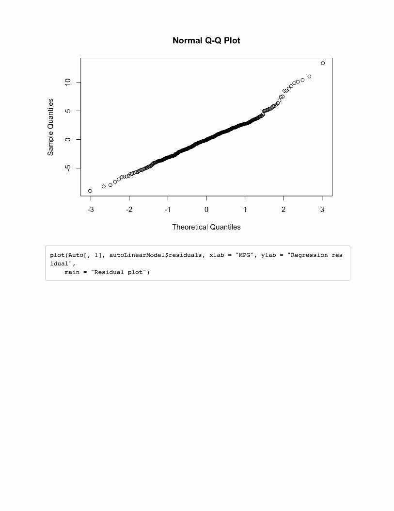
The first plot, a normal quantile-quantile plot of the regression residuals, shows that the residuals areapproximately normally distributed and that there are no extremely surprising outliers. However, theother plot, the residual plot, shows a problem with the fit of the model. There is a dependencebetween the response (MPG) and the residual. For small and large MPGs, the model seems tounderestimate, and for MPGs in the middle, the model seems to overestimate.

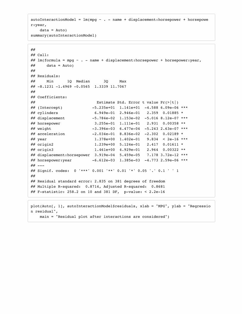
e. In this setting, there are (72)=32 pairwise interactions to consider. Hence there are235=34359738368 choices of “models with interaction effects” (more if you consider three-wayinteractions, four-way interactions, etc.). It is not feasible to consider such a large set of models,so we can approach this problem in a greedy fashion: Consider all 35 pairwise interactions andinclude the one with the largest (standardized) effect. Then consider the remaining 34 pairwiseinteractions and again include the one with the largest effect. You could do this repeatedly untilthe effects being added to the linear model are no longer significant.

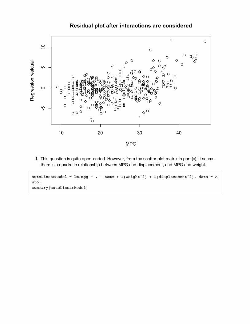
In this problem, the most significant interaction is between displacement and horsepower. Once thatinteraction is included in the model, the next most significant interaction is between horsepower andyear. One could continue from there, but the next interaction is of dubious significance. To answer thequestion posed by the textbook, yes, there are definitely interactions that appear to be significant.However, including these interaction terms does not entirely fix (see plot below) the diagnosticproblem from part (d). In order to fix this problem, one should think critically about a physical model forgas consumption and intelligently choose transformations of the variables to reflect this, as the nextpart of this exercise is getting at.

autoInteractionModel = lm(mpg ~ . - name + displacement:horsepower + horsepower:year, data = Auto)summary(autoInteractionModel)

## ## Call:## lm(formula = mpg ~ . - name + displacement:horsepower + horsepower:year, ## data = Auto)## ## Residuals:## Min 1Q Median 3Q Max ## -8.1231 -1.4969 -0.0565 1.3339 11.7067 ## ## Coefficients:## Estimate Std. Error t value Pr(>|t|) ## (Intercept) -5.235e+01 1.141e+01 -4.588 6.09e-06 ***## cylinders 6.949e-01 2.946e-01 2.359 0.01885 * ## displacement -5.784e-02 1.153e-02 -5.016 8.12e-07 ***## horsepower 3.255e-01 1.111e-01 2.931 0.00358 ** ## weight -3.396e-03 6.477e-04 -5.243 2.63e-07 ***## acceleration -2.034e-01 8.836e-02 -2.302 0.02189 * ## year 1.378e+00 1.402e-01 9.834 < 2e-16 ***## origin2 1.239e+00 5.124e-01 2.417 0.01611 * ## origin3 1.461e+00 4.929e-01 2.964 0.00322 ** ## displacement:horsepower 3.919e-04 5.459e-05 7.178 3.72e-12 ***## horsepower:year -6.612e-03 1.385e-03 -4.773 2.59e-06 ***## ---## Signif. codes: 0 '***' 0.001 '**' 0.01 '*' 0.05 '.' 0.1 ' ' 1## ## Residual standard error: 2.835 on 381 degrees of freedom## Multiple R-squared: 0.8714, Adjusted R-squared: 0.8681 ## F-statistic: 258.2 on 10 and 381 DF, p-value: < 2.2e-16

plot(Auto[, 1], autoInteractionModel$residuals, xlab = "MPG", ylab = "Regression residual", main = "Residual plot after interactions are considered")

f. This question is quite open-ended. However, from the scatter plot matrix in part (a), it seems

there is a quadratic relationship between MPG and displacement, and MPG and weight.

autoLinearModel = lm(mpg ~ . - name + I(weight^2) + I(displacement^2), data = Auto)summary(autoLinearModel)

Both of the quadratic terms included appear to be significant and improve the R2 and adjusted R2statistics.

Problem 7 (3.14)a) The form of the linear model is for , where i.i.d.

. In this case, the regression coefficients are , and .

set.seed(1) # We set the seed to obtain the same result# every time the script is run.x1 = runif(100)x2 = 0.5 * x1 + rnorm(100)/10y = 2 + 2 * x1 + 0.3 * x2 + rnorm(100)

b.

cor(x1, x2)

## [1] 0.8351212

plot(x1, x2, main = "Scatterplot of x1 and x2")

## ## Call:## lm(formula = mpg ~ . - name + I(weight^2) + I(displacement^2), ## data = Auto)## ## Residuals:## Min 1Q Median 3Q Max ## -9.5345 -1.7279 0.0206 1.6162 12.3679 ## ## Coefficients:## Estimate Std. Error t value Pr(>|t|) ## (Intercept) -2.232e+00 4.648e+00 -0.480 0.63138 ## cylinders 2.048e-01 3.353e-01 0.611 0.54171 ## displacement -3.950e-02 2.139e-02 -1.847 0.06557 . ## horsepower -4.184e-02 1.356e-02 -3.085 0.00218 ** ## weight -1.476e-02 2.600e-03 -5.678 2.70e-08 ***## acceleration 2.136e-02 8.890e-02 0.240 0.81029 ## year 8.034e-01 4.697e-02 17.106 < 2e-16 ***## origin2 1.195e+00 5.619e-01 2.127 0.03409 * ## origin3 1.003e+00 5.413e-01 1.853 0.06465 . ## I(weight^2) 1.468e-06 3.540e-07 4.147 4.16e-05 ***## I(displacement^2) 9.662e-05 3.435e-05 2.813 0.00516 ** ## ---## Signif. codes: 0 '***' 0.001 '**' 0.01 '*' 0.05 '.' 0.1 ' ' 1## ## Residual standard error: 2.948 on 381 degrees of freedom## Multiple R-squared: 0.861, Adjusted R-squared: 0.8574 ## F-statistic: 236 on 10 and 381 DF, p-value: < 2.2e-16

c)

summary(lm(y ~ x1 + x2))

## ## Call:## lm(formula = y ~ x1 + x2)## ## Residuals:## Min 1Q Median 3Q Max ## -2.8311 -0.7273 -0.0537 0.6338 2.3359 ## ## Coefficients:## Estimate Std. Error t value Pr(>|t|) ## (Intercept) 2.1305 0.2319 9.188 7.61e-15 ***## x1 1.4396 0.7212 1.996 0.0487 * ## x2 1.0097 1.1337 0.891 0.3754 ## ---## Signif. codes: 0 '***' 0.001 '**' 0.01 '*' 0.05 '.' 0.1 ' ' 1## ## Residual standard error: 1.056 on 97 degrees of freedom## Multiple R-squared: 0.2088, Adjusted R-squared: 0.1925 ## F-statistic: 12.8 on 2 and 97 DF, p-value: 1.164e-05

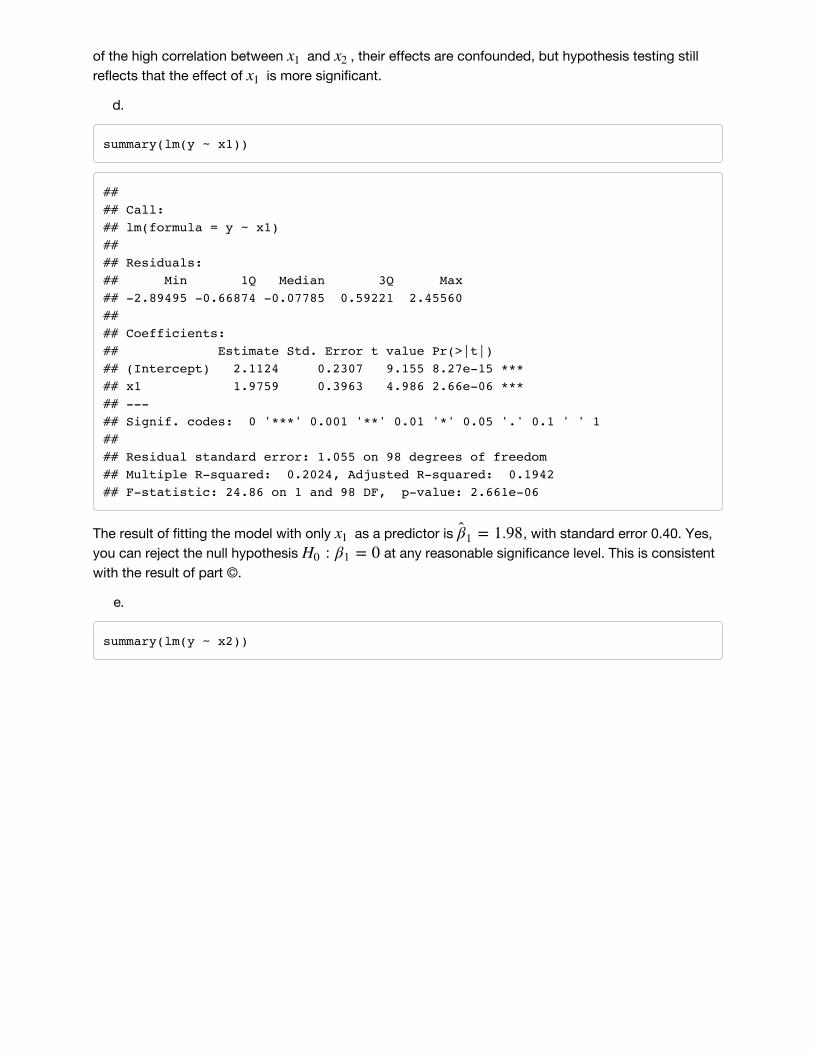
The result of fitting the model is , and . The estimate of (2) is close,but the estimate of (2) is too low, and the estimate of (0.3) is too high. At -level .05, you canreject the null hypothesis but not the null hypothesis . It seems that because

of the high correlation between and , their effects are confounded, but hypothesis testing stillreflects that the effect of is more significant.

d.

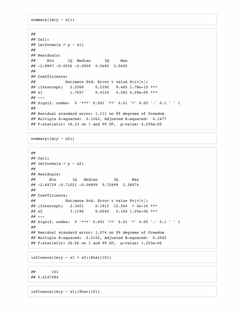
summary(lm(y ~ x1))

## ## Call:## lm(formula = y ~ x1)## ## Residuals:## Min 1Q Median 3Q Max ## -2.89495 -0.66874 -0.07785 0.59221 2.45560 ## ## Coefficients:## Estimate Std. Error t value Pr(>|t|) ## (Intercept) 2.1124 0.2307 9.155 8.27e-15 ***## x1 1.9759 0.3963 4.986 2.66e-06 ***## ---## Signif. codes: 0 '***' 0.001 '**' 0.01 '*' 0.05 '.' 0.1 ' ' 1## ## Residual standard error: 1.055 on 98 degrees of freedom## Multiple R-squared: 0.2024, Adjusted R-squared: 0.1942 ## F-statistic: 24.86 on 1 and 98 DF, p-value: 2.661e-06

The result of fitting the model with only as a predictor is , with standard error 0.40. Yes,you can reject the null hypothesis at any reasonable significance level. This is consistentwith the result of part ©.

e.

summary(lm(y ~ x2))

## ## Call:## lm(formula = y ~ x2)## ## Residuals:## Min 1Q Median 3Q Max ## -2.62687 -0.75156 -0.03598 0.72383 2.44890 ## ## Coefficients:## Estimate Std. Error t value Pr(>|t|) ## (Intercept) 2.3899 0.1949 12.26 < 2e-16 ***## x2 2.8996 0.6330 4.58 1.37e-05 ***## ---## Signif. codes: 0 '***' 0.001 '**' 0.01 '*' 0.05 '.' 0.1 ' ' 1## ## Residual standard error: 1.072 on 98 degrees of freedom## Multiple R-squared: 0.1763, Adjusted R-squared: 0.1679 ## F-statistic: 20.98 on 1 and 98 DF, p-value: 1.366e-05

The result of fitting the model with only as a predictor is , with standard error 0.63. Yes,you can reject the null hypothesis at any reasonable significance level. This is notconsistent with the result of part ©.

f. The result of part (e) is contradictory to the result of part (c) and shows how the significance testfor one variable can be affected by the inclusion of another variable in the model.

g.

x1 = c(x1, 0.1)x2 = c(x2, 0.8)y = c(y, 6)summary(lm(y ~ x1 + x2))

## ## Call:## lm(formula = y ~ x1 + x2)## ## Residuals:## Min 1Q Median 3Q Max ## -2.73348 -0.69318 -0.05263 0.66385 2.30619 ## ## Coefficients:## Estimate Std. Error t value Pr(>|t|) ## (Intercept) 2.2267 0.2314 9.624 7.91e-16 ***## x1 0.5394 0.5922 0.911 0.36458 ## x2 2.5146 0.8977 2.801 0.00614 ** ## ---## Signif. codes: 0 '***' 0.001 '**' 0.01 '*' 0.05 '.' 0.1 ' ' 1## ## Residual standard error: 1.075 on 98 degrees of freedom## Multiple R-squared: 0.2188, Adjusted R-squared: 0.2029 ## F-statistic: 13.72 on 2 and 98 DF, p-value: 5.564e-06

summary(lm(y ~ x1))

## ## Call:## lm(formula = y ~ x1)## ## Residuals:## Min 1Q Median 3Q Max ## -2.8897 -0.6556 -0.0909 0.5682 3.5665 ## ## Coefficients:## Estimate Std. Error t value Pr(>|t|) ## (Intercept) 2.2569 0.2390 9.445 1.78e-15 ***## x1 1.7657 0.4124 4.282 4.29e-05 ***## ---## Signif. codes: 0 '***' 0.001 '**' 0.01 '*' 0.05 '.' 0.1 ' ' 1## ## Residual standard error: 1.111 on 99 degrees of freedom## Multiple R-squared: 0.1562, Adjusted R-squared: 0.1477 ## F-statistic: 18.33 on 1 and 99 DF, p-value: 4.295e-05

summary(lm(y ~ x2))

## ## Call:## lm(formula = y ~ x2)## ## Residuals:## Min 1Q Median 3Q Max ## -2.64729 -0.71021 -0.06899 0.72699 2.38074 ## ## Coefficients:## Estimate Std. Error t value Pr(>|t|) ## (Intercept) 2.3451 0.1912 12.264 < 2e-16 ***## x2 3.1190 0.6040 5.164 1.25e-06 ***## ---## Signif. codes: 0 '***' 0.001 '**' 0.01 '*' 0.05 '.' 0.1 ' ' 1## ## Residual standard error: 1.074 on 99 degrees of freedom## Multiple R-squared: 0.2122, Adjusted R-squared: 0.2042 ## F-statistic: 26.66 on 1 and 99 DF, p-value: 1.253e-06

influence(lm(y ~ x1 + x2))$hat[101]

## 101 ## 0.4147284

influence(lm(y ~ x1))$hat[101]

## 101 ## 0.03347156

influence(lm(y ~ x2))$hat[101]

## 101 ## 0.1013106

Introducing the mis-measured observation does not change the hypothesis testing result of either of

the single-predictor regressions, but in the full regression, the significance is switched: You can reject

the null hypothesis but not the null hypothesis . Inspection of the histograms

of the three variables reveals that the new observation is not an outlier in any of the three models.

However, this observation is a point of high leverage in the full regression model (leverage statistic

) and the regression model with just as a predictor ( ), not in the regression

model with just as a predictor ( ).

Problem 8 (3.15)

library(MASS)

a. We ran simple linear regressions with the following commands (output suppressed). The

response has a significant relationship with all predictors except chad.

summary(lm(crim ~ zn, data = Boston))summary(lm(crim ~ indus, data = Boston))summary(lm(crim ~ chas, data = Boston))summary(lm(crim ~ nox, data = Boston))summary(lm(crim ~ rm, data = Boston))summary(lm(crim ~ age, data = Boston))summary(lm(crim ~ dis, data = Boston))summary(lm(crim ~ rad, data = Boston))summary(lm(crim ~ tax, data = Boston))summary(lm(crim ~ ptratio, data = Boston))summary(lm(crim ~ black, data = Boston))summary(lm(crim ~ lstat, data = Boston))summary(lm(crim ~ medv, data = Boston))

b) The predictors for which we can reject the null hypothesis at significance level .05 are

zn, dis, rad, black and medv.

summary(lm(crim ~ ., data = Boston))

## ## Call:## lm(formula = crim ~ ., data = Boston)## ## Residuals:## Min 1Q Median 3Q Max ## -9.924 -2.120 -0.353 1.019 75.051 ## ## Coefficients:## Estimate Std. Error t value Pr(>|t|) ## (Intercept) 17.033228 7.234903 2.354 0.018949 * ## zn 0.044855 0.018734 2.394 0.017025 * ## indus -0.063855 0.083407 -0.766 0.444294 ## chas -0.749134 1.180147 -0.635 0.525867 ## nox -10.313535 5.275536 -1.955 0.051152 . ## rm 0.430131 0.612830 0.702 0.483089 ## age 0.001452 0.017925 0.081 0.935488 ## dis -0.987176 0.281817 -3.503 0.000502 ***## rad 0.588209 0.088049 6.680 6.46e-11 ***## tax -0.003780 0.005156 -0.733 0.463793 ## ptratio -0.271081 0.186450 -1.454 0.146611 ## black -0.007538 0.003673 -2.052 0.040702 * ## lstat 0.126211 0.075725 1.667 0.096208 . ## medv -0.198887 0.060516 -3.287 0.001087 ** ## ---## Signif. codes: 0 '***' 0.001 '**' 0.01 '*' 0.05 '.' 0.1 ' ' 1## ## Residual standard error: 6.439 on 492 degrees of freedom## Multiple R-squared: 0.454, Adjusted R-squared: 0.4396 ## F-statistic: 31.47 on 13 and 492 DF, p-value: < 2.2e-16

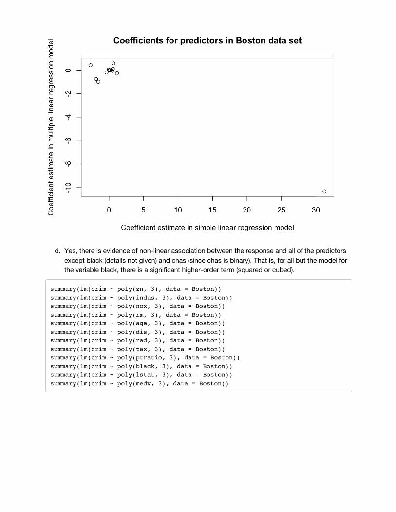
c)The results are quite different, which makes sense because including a large number of additionalpredictors can change the estimated effect of each predictor.

y = lm(crim ~ ., data = Boston)$coef[2:14]x = c(-0.073, 0.51, -1.893, 31.249, -2.684, 0.108, -1.551, 0.618, 0.03, 1.152, -0.036, 0.549, -0.363)plot(x, y, xlab = "Coefficient estimate in simple linear regression model", ylab = "Coefficient estimate in multiple linear regression model", main = "Coefficients for predictors in Boston data set")

d. Yes, there is evidence of non-linear association between the response and all of the predictorsexcept black (details not given) and chas (since chas is binary). That is, for all but the model forthe variable black, there is a significant higher-order term (squared or cubed).

summary(lm(crim ~ poly(zn, 3), data = Boston))summary(lm(crim ~ poly(indus, 3), data = Boston))summary(lm(crim ~ poly(nox, 3), data = Boston))summary(lm(crim ~ poly(rm, 3), data = Boston))summary(lm(crim ~ poly(age, 3), data = Boston))summary(lm(crim ~ poly(dis, 3), data = Boston))summary(lm(crim ~ poly(rad, 3), data = Boston))summary(lm(crim ~ poly(tax, 3), data = Boston))summary(lm(crim ~ poly(ptratio, 3), data = Boston))summary(lm(crim ~ poly(black, 3), data = Boston))summary(lm(crim ~ poly(lstat, 3), data = Boston))summary(lm(crim ~ poly(medv, 3), data = Boston))

Problem 91. First, we setup the data.

Question 4a.

X <- matrix(rnorm(3000), 60, 50)X[1:20, 1] <- X[1:20, 1] + 4;X[21:40, 1] <- X[21:40, 1] - 4;

X[1:20, 2] <- X[1:20, 1] + 4;X[21:40, 2] <- X[21:40, 1] - 4;

b.

pca = prcomp(X)summary(pca)

## Importance of components:## PC1 PC2 PC3 PC4 PC5 PC6## Standard deviation 7.4017 1.9492 1.79083 1.71476 1.67233 1.63812## Proportion of Variance 0.5205 0.0361 0.03047 0.02793 0.02657 0.02549## Cumulative Proportion 0.5205 0.5566 0.58704 0.61498 0.64155 0.66704## PC7 PC8 PC9 PC10 PC11 PC12## Standard deviation 1.54143 1.51214 1.47083 1.40467 1.3991 1.3727## Proportion of Variance 0.02257 0.02172 0.02055 0.01875 0.0186 0.0179## Cumulative Proportion 0.68961 0.71134 0.73189 0.75064 0.7692 0.7871## PC13 PC14 PC15 PC16 PC17 PC18## Standard deviation 1.31985 1.24097 1.21163 1.1833 1.1606 1.10798## Proportion of Variance 0.01655 0.01463 0.01395 0.0133 0.0128 0.01166## Cumulative Proportion 0.80368 0.81831 0.83226 0.8456 0.8584 0.87002## PC19 PC20 PC21 PC22 PC23 PC24## Standard deviation 1.08057 1.06285 1.03186 0.96037 0.92612 0.9000## Proportion of Variance 0.01109 0.01073 0.01012 0.00876 0.00815 0.0077## Cumulative Proportion 0.88112 0.89185 0.90196 0.91073 0.91888 0.9266## PC25 PC26 PC27 PC28 PC29 PC30## Standard deviation 0.8584 0.82377 0.81513 0.79853 0.76326 0.73840## Proportion of Variance 0.0070 0.00645 0.00631 0.00606 0.00553 0.00518## Cumulative Proportion 0.9336 0.94002 0.94633 0.95239 0.95792 0.96310## PC31 PC32 PC33 PC34 PC35 PC36## Standard deviation 0.71328 0.63926 0.58763 0.57476 0.55882 0.53012## Proportion of Variance 0.00483 0.00388 0.00328 0.00314 0.00297 0.00267## Cumulative Proportion 0.96794 0.97182 0.97510 0.97824 0.98120 0.98387## PC37 PC38 PC39 PC40 PC41 PC42## Standard deviation 0.52050 0.4923 0.45681 0.44048 0.40283 0.35663## Proportion of Variance 0.00257 0.0023 0.00198 0.00184 0.00154 0.00121## Cumulative Proportion 0.98645 0.9888 0.99073 0.99258 0.99412 0.99533## PC43 PC44 PC45 PC46 PC47 PC48## Standard deviation 0.34336 0.31146 0.28258 0.27698 0.22234 0.19458## Proportion of Variance 0.00112 0.00092 0.00076 0.00073 0.00047 0.00036## Cumulative Proportion 0.99645 0.99737 0.99813 0.99886 0.99932 0.99968## PC49 PC50## Standard deviation 0.17127 0.06217## Proportion of Variance 0.00028 0.00004## Cumulative Proportion 0.99996 1.00000

Y = pca$x[,1:2]plot(Y, col=c(rep(1,20), rep(2,20), rep(3,20)), xlab="Z1", ylab="Z2", pch=19)

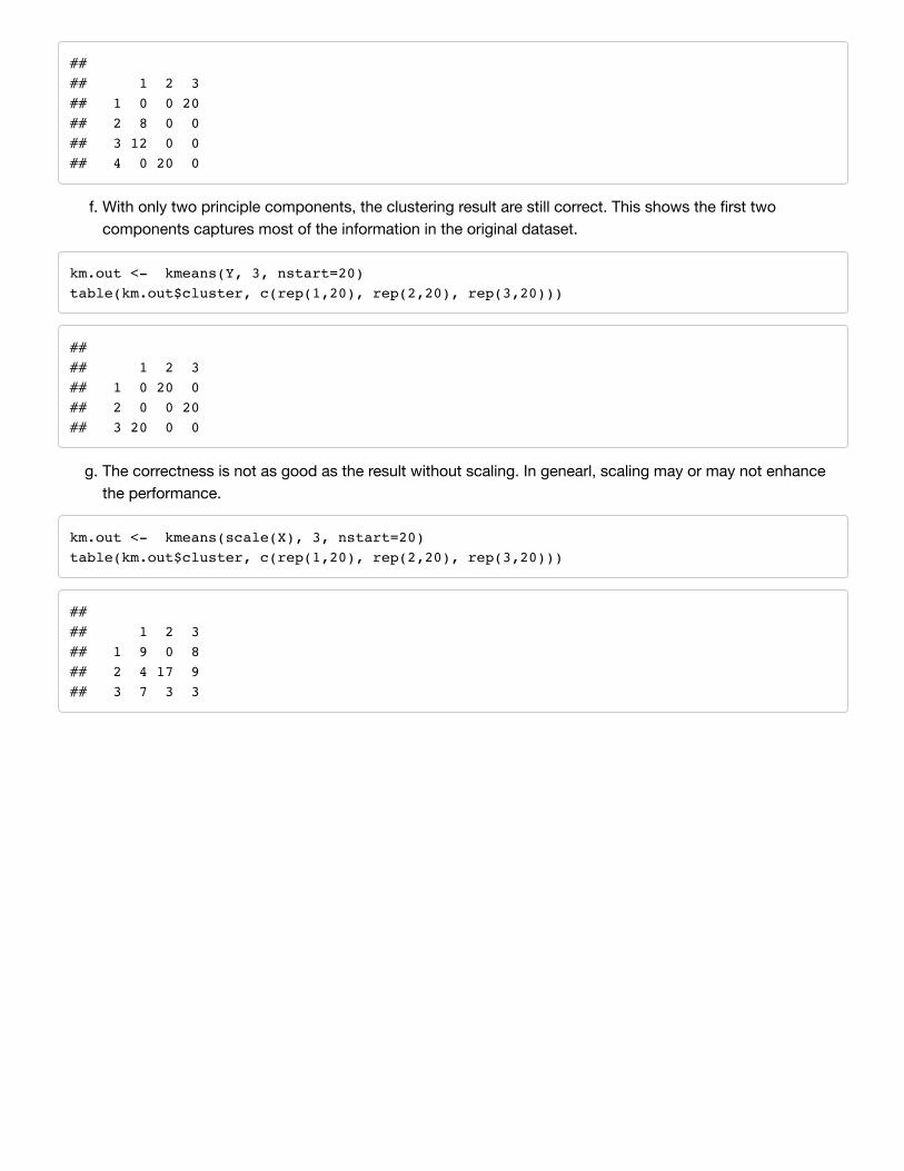
(c)(d)(e) For , K-means does a good job and all points are clustered in the correct group. For , K-means seperates one of the cluster into two. For , K-means combines two clusters into one.

km.out <- kmeans(X, 3, nstart=20)table(km.out$cluster, c(rep(1,20), rep(2,20), rep(3,20)))

## ## 1 2 3## 1 0 20 0## 2 0 0 20## 3 20 0 0

km.out <- kmeans(X, 2, nstart=20)table(km.out$cluster, c(rep(1,20), rep(2,20), rep(3,20)))

## ## 1 2 3## 1 20 0 20## 2 0 20 0

km.out <- kmeans(X, 4, nstart=20)table(km.out$cluster, c(rep(1,20), rep(2,20), rep(3,20)))

## ## 1 2 3## 1 0 0 20## 2 8 0 0## 3 12 0 0## 4 0 20 0

f. With only two principle components, the clustering result are still correct. This shows the first twocomponents captures most of the information in the original dataset.

km.out <- kmeans(Y, 3, nstart=20)table(km.out$cluster, c(rep(1,20), rep(2,20), rep(3,20)))

## ## 1 2 3## 1 0 20 0## 2 0 0 20## 3 20 0 0

g. The correctness is not as good as the result without scaling. In genearl, scaling may or may not enhancethe performance.

km.out <- kmeans(scale(X), 3, nstart=20)table(km.out$cluster, c(rep(1,20), rep(2,20), rep(3,20)))

## ## 1 2 3## 1 9 0 8## 2 4 17 9## 3 7 3 3