Projects 3-4 person groups preferred Deliverables: Poster & Report & main code (plus proposal, midterm slide) Topics your own or chose form suggested topics. Some physics/engineering inspired. April 26 groups due to TA (if you don’t have a group, ask in piazza we can help). TAs will construct groups after that. May 5 proposal due. TAs and Peter can approve. Proposal: One page: Title, a large paragraph, data, weblinks, references. May 20 Midterm slide presentation. Presented to a subgroup of class. June 5 final poster. Uploaded June 3 Report and code due Saturday 15 June. Q: Can the final project be shared with another class? If the other class allows it it should be fine. You cannot turn in an identical project for both classes, but you can share common infrastructure/code base/datasets across the two classes. No cut and paste from other sources without making clear that this part is a copy. This applies to other reports or things from internet. Citations are important. Homework Sunday CNN lecture Mockdag
Transcript
Projects3-4 person groups preferredDeliverables: Poster & Report & main code (plus proposal, midterm slide)
Topics your own or chose form suggested topics. Some physics/engineering inspired.
April 26 groups due to TA (if you don’t have a group, ask in piazza we can help). TAs will construct groups after that.
May 5 proposal due. TAs and Peter can approve. Proposal: One page: Title, a large paragraph, data, weblinks, references.
May 20 Midterm slide presentation. Presented to a subgroup of class.
June 5 final poster. Uploaded June 3Report and code due Saturday 15 June.Q: Can the final project be shared with another class?If the other class allows it it should be fine. You cannot turn in an identical project for both classes, but you can share common infrastructure/code base/datasets across the two classes.
No cut and paste from other sources without making clear that this part is a copy. This applies to other reports or things from internet. Citations are important.
HomeworkSundayCNN lecture Mockdag
Fei-Fei Li & Justin Johnson & Serena Yeung Lecture 7 - April 25, 2017Fei-Fei Li & Justin Johnson & Serena Yeung Lecture 7 - April 25, 20179
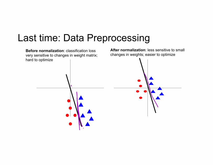
Last time: Data PreprocessingBefore normalization: classification loss very sensitive to changes in weight matrix; hard to optimize
After normalization: less sensitive to small changes in weights; easier to optimize
I
l
Fei-Fei Li & Justin Johnson & Serena Yeung Lecture 7 - April 25, 2017Fei-Fei Li & Justin Johnson & Serena Yeung Lecture 7 - April 25, 201716
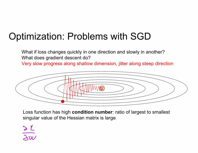
Optimization: Problems with SGDWhat if loss changes quickly in one direction and slowly in another?What does gradient descent do?Very slow progress along shallow dimension, jitter along steep direction
Loss function has high condition number: ratio of largest to smallest singular value of the Hessian matrix is large
S LJw
Fei-Fei Li & Justin Johnson & Serena Yeung Lecture 7 - April 25, 2017Fei-Fei Li & Justin Johnson & Serena Yeung Lecture 7 - April 25, 201718
Optimization: Problems with SGD
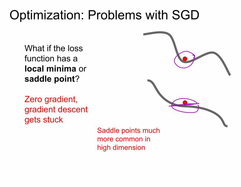
What if the loss function has a local minima or saddle point?
Zero gradient, gradient descent gets stuck
Fei-Fei Li & Justin Johnson & Serena Yeung Lecture 7 - April 25, 2017Fei-Fei Li & Justin Johnson & Serena Yeung Lecture 7 - April 25, 201719
Optimization: Problems with SGD
What if the loss function has a local minima or saddle point?
Saddle points much more common in high dimension
Dauphin et al, “Identifying and attacking the saddle point problem in high-dimensional non-convex optimization”, NIPS 2014
Fei-Fei Li & Justin Johnson & Serena Yeung Lecture 7 - April 25, 2017Fei-Fei Li & Justin Johnson & Serena Yeung Lecture 7 - April 25, 201720
Optimization: Problems with SGD
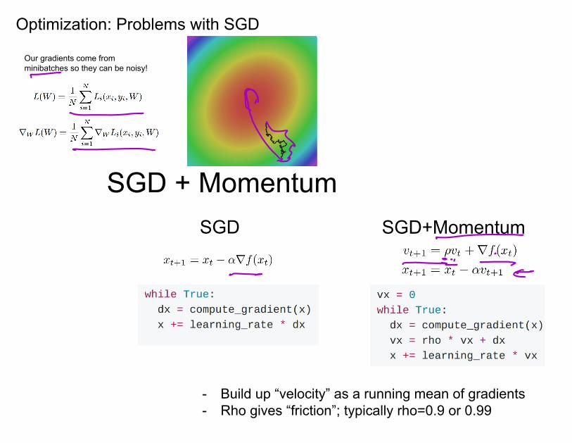
Our gradients come from minibatches so they can be noisy!
Fei-Fei Li & Justin Johnson & Serena Yeung Lecture 7 - April 25, 2017Fei-Fei Li & Justin Johnson & Serena Yeung Lecture 7 - April 25, 201721
SGD + MomentumSGD SGD+Momentum
- Build up “velocity” as a running mean of gradients- Rho gives “friction”; typically rho=0.9 or 0.99
es
Fei-Fei Li & Justin Johnson & Serena Yeung Lecture 7 - April 25, 2017Fei-Fei Li & Justin Johnson & Serena Yeung Lecture 7 - April 25, 201737
Adam (full form)
Kingma and Ba, “Adam: A method for stochastic optimization”, ICLR 2015
Momentum
AdaGrad / RMSProp
Bias correction
Bias correction for the fact that first and second moment estimates start at zero
Adam with beta1 = 0.9, beta2 = 0.999, and learning_rate = 1e-3 or 5e-4is a great starting point for many models!
4
Fei-Fei Li & Justin Johnson & Serena Yeung Lecture 7 - April 25, 2017Fei-Fei Li & Justin Johnson & Serena Yeung Lecture 7 - April 25, 201740
SGD, SGD+Momentum, Adagrad, RMSProp, Adam all have learning rate as a hyperparameter.
=> Learning rate decay over time!
step decay: e.g. decay learning rate by half every few epochs.
exponential decay:
1/t decay:
Fei-Fei Li & Justin Johnson & Serena Yeung Lecture 7 - April 25, 2017Fei-Fei Li & Justin Johnson & Serena Yeung Lecture 7 - April 25, 201758
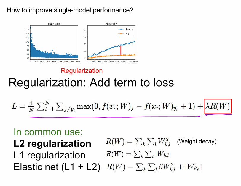
How to improve single-model performance?
Regularization
Fei-Fei Li & Justin Johnson & Serena Yeung Lecture 7 - April 25, 2017Fei-Fei Li & Justin Johnson & Serena Yeung Lecture 7 - April 25, 2017
Regularization: Add term to loss
59
In common use: L2 regularizationL1 regularizationElastic net (L1 + L2)
(Weight decay)
Fei-Fei Li & Justin Johnson & Serena Yeung Lecture 7 - April 25, 2017Fei-Fei Li & Justin Johnson & Serena Yeung Lecture 7 - April 25, 201760
Regularization: DropoutIn each forward pass, randomly set some neurons to zeroProbability of dropping is a hyperparameter; 0.5 is common
Srivastava et al, “Dropout: A simple way to prevent neural networks from overfitting”, JMLR 2014
Homework
Fei-Fei Li & Justin Johnson & Serena Yeung Lecture 7 - April 25, 2017Fei-Fei Li & Justin Johnson & Serena Yeung Lecture 7 - April 25, 201762
Regularization: DropoutHow can this possibly be a good idea?
Forces the network to have a redundant representation;Prevents co-adaptation of features
has an ear
has a tail
is furry
has claws
mischievous look
cat score
X
X
X
Fei-Fei Li & Justin Johnson & Serena Yeung Lecture 7 - April 25, 2017Fei-Fei Li & Justin Johnson & Serena Yeung Lecture 7 - April 25, 201775
Regularization: Data Augmentation
Load image and label
“cat”
CNN
Computeloss
Transform image
Fei-Fei Li & Justin Johnson & Serena Yeung Lecture 7 - April 25, 2017Fei-Fei Li & Justin Johnson & Serena Yeung Lecture 7 - April 25, 201781
Data AugmentationGet creative for your problem!
Random mix/combinations of :- translation- rotation- stretching- shearing, - lens distortions, … (go crazy)
+simulated data using physical model.
true
Fei-Fei Li & Justin Johnson & Serena Yeung Lecture 7 - April 25, 2017Fei-Fei Li & Justin Johnson & Serena Yeung Lecture 7 - April 25, 201790
Transfer Learning with CNNs
Image
Conv-64Conv-64MaxPool
Conv-128Conv-128MaxPool
Conv-256Conv-256MaxPool
Conv-512Conv-512MaxPool
Conv-512Conv-512MaxPool
FC-4096FC-4096FC-1000
1. Train on Imagenet
Image
Conv-64Conv-64MaxPool
Conv-128Conv-128MaxPool
Conv-256Conv-256MaxPool
Conv-512Conv-512MaxPool
Conv-512Conv-512MaxPool
FC-4096FC-4096FC-C
2. Small Dataset (C classes)
Freeze these
Reinitialize this and train
Image
Conv-64Conv-64MaxPool
Conv-128Conv-128MaxPool
Conv-256Conv-256MaxPool
Conv-512Conv-512MaxPool
Conv-512Conv-512MaxPool
FC-4096FC-4096FC-C
3. Bigger dataset
Freeze these
Train these
With bigger dataset, train more layers
Lower learning rate when finetuning; 1/10 of original LR is good starting point
Donahue et al, “DeCAF: A Deep Convolutional Activation Feature for Generic Visual Recognition”, ICML 2014Razavian et al, “CNN Features Off-the-Shelf: An Astounding Baseline for Recognition”, CVPR Workshops 2014
8
Predicting Weather with Machine Learning:
Intro to ARMA and Random Forest
Emma OzanichPhD Candidate,
Scripps Institution of Oceanography
BackgroundShi et al NIPS 2015 –• Predicting rain at different time
lags• Shows convolutional lstm vs
nowcast models vs fully-connected lstm
• Used radar echo (image) inputso Hong Kong, 2011-2013, o 240 frames/dayo Selected top 97 rainy dayso Note: <10% of data used!
• Preprocessing: k-means clustering to denoise
• ConvLSTM has better performance and lower false alarm (lower left)
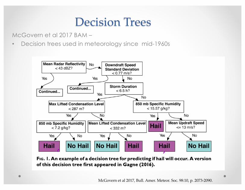
BackgroundMcGovern et al 2017 BAM –• Decision trees used in meteorology since mid-1960s
McGovern et al 2017, Bull. Amer. Meteor. Soc. 98:10, p. 2073-2090.
Predicting rain at different time lagsx
BackgroundMcGovern et al 2017 BAM –• Green contours = hail occurred (truth)• Physics based method: Convection-allowing model (CAM)
o Doesn’t directly predict hail• Random forest predicts hail size (Γ) distribution based on weather• HAILCAST = diagnostic measure based on CAMs• Updraft Helicity = surrogate variable from CAM
McGovern et al 2017, Bull. Amer. Meteor. Soc. 98:10, p. 2073-2090.
it
0
Decision Trees• Algorithm made up of conditional control statements
Homework'Deadline'tonight?'
Do'homework'
Yes'
Party'invitaNon?'
No'
No'
Do'I'have'friends'
Yes'
Go'to'the'party'
Read'a'book'
No'Hang'out'with'
friends'
Yes'
n
p
Decision TreesMcGovern et al 2017 BAM –• Decision trees used in meteorology since mid-1960s
McGovern et al 2017, Bull. Amer. Meteor. Soc. 98:10, p. 2073-2090.
I e
|
t1
t2
t3
t4
R1
R1
R2
R2
R3
R3
R4
R4
R5
R5
X1
X1X1
X2
X2
X2
X1 ≤ t1
X2 ≤ t2 X1 ≤ t3
X2 ≤ t4
• Divide data into distinct, non-overlapping regions R1,…, RJ
• Below yi = color = continuous target (<blue = 1 and >red = 0). • xi , i = 1,..,5 samples• !" = $%, $' , with P = 2 features.• j = 1,..,5 (5 regions).
Regression Tree
Hastie et al 2017, Chap. 9 p 307.
|
t1
t2
t3
t4
R1
R1
R2
R2
R3
R3
R4
R4
R5
R5
X1
X1X1
X2
X2
X2
X1 ≤ t1
X2 ≤ t2 X1 ≤ t3
X2 ≤ t4
Tree-building• Or, consecutively partition a region into non-overlapping
rectangles• yi = color = continuous target (<blue = 1 and >red = 0). • xi , i = 1,..,5 samples• !" = $%, $' , with P = 2 features.• j = 1,..,5 (5 regions).
Hastie et al 2017, Chap. 9 p 307.
41
|
t1
t2
t3
t4
R1
R1
R2
R2
R3
R3
R4
R4
R5
R5
X1
X1X1
X2
X2
X2
X1 ≤ t1
X2 ≤ t2 X1 ≤ t3
X2 ≤ t4
R2
Regression Tree• How to optimize a regression tree?• Randomly select t1
• Assign region labels:
o Example-
9.2 Tree-Based Methods 307
population into strata of high and low outcome, on the basis of patientcharacteristics.
9.2.2 Regression Trees
We now turn to the question of how to grow a regression tree. Our dataconsists of p inputs and a response, for each of N observations: that is,(xi, yi) for i = 1, 2, . . . , N , with xi = (xi1, xi2, . . . , xip). The algorithmneeds to automatically decide on the splitting variables and split points,and also what topology (shape) the tree should have. Suppose first that wehave a partition intoM regions R1, R2, . . . , RM , and we model the responseas a constant cm in each region:
f(x) =M!
m=1
cmI(x ∈ Rm). (9.10)
If we adopt as our criterion minimization of the sum of squares"
(yi −f(xi))2, it is easy to see that the best cm is just the average of yi in regionRm:
cm = ave(yi|xi ∈ Rm). (9.11)
Now finding the best binary partition in terms of minimum sum of squaresis generally computationally infeasible. Hence we proceed with a greedyalgorithm. Starting with all of the data, consider a splitting variable j andsplit point s, and define the pair of half-planes
For each splitting variable, the determination of the split point s canbe done very quickly and hence by scanning through all of the inputs,determination of the best pair (j, s) is feasible.Having found the best split, we partition the data into the two resulting
regions and repeat the splitting process on each of the two regions. Thenthis process is repeated on all of the resulting regions.
How large should we grow the tree? Clearly a very large tree might overfitthe data, while a small tree might not capture the important structure.
t1
t1
9.2 Tree-Based Methods 307
population into strata of high and low outcome, on the basis of patientcharacteristics.
9.2.2 Regression Trees
We now turn to the question of how to grow a regression tree. Our dataconsists of p inputs and a response, for each of N observations: that is,(xi, yi) for i = 1, 2, . . . , N , with xi = (xi1, xi2, . . . , xip). The algorithmneeds to automatically decide on the splitting variables and split points,and also what topology (shape) the tree should have. Suppose first that wehave a partition intoM regions R1, R2, . . . , RM , and we model the responseas a constant cm in each region:
f(x) =M!
m=1
cmI(x ∈ Rm). (9.10)
If we adopt as our criterion minimization of the sum of squares"
(yi −f(xi))2, it is easy to see that the best cm is just the average of yi in regionRm:
cm = ave(yi|xi ∈ Rm). (9.11)
Now finding the best binary partition in terms of minimum sum of squaresis generally computationally infeasible. Hence we proceed with a greedyalgorithm. Starting with all of the data, consider a splitting variable j andsplit point s, and define the pair of half-planes
For each splitting variable, the determination of the split point s canbe done very quickly and hence by scanning through all of the inputs,determination of the best pair (j, s) is feasible.Having found the best split, we partition the data into the two resulting
regions and repeat the splitting process on each of the two regions. Thenthis process is repeated on all of the resulting regions.
How large should we grow the tree? Clearly a very large tree might overfitthe data, while a small tree might not capture the important structure.
, j = 1
t1
t1
9.2 Tree-Based Methods 307
population into strata of high and low outcome, on the basis of patientcharacteristics.
9.2.2 Regression Trees
We now turn to the question of how to grow a regression tree. Our dataconsists of p inputs and a response, for each of N observations: that is,(xi, yi) for i = 1, 2, . . . , N , with xi = (xi1, xi2, . . . , xip). The algorithmneeds to automatically decide on the splitting variables and split points,and also what topology (shape) the tree should have. Suppose first that wehave a partition intoM regions R1, R2, . . . , RM , and we model the responseas a constant cm in each region:
f(x) =M!
m=1
cmI(x ∈ Rm). (9.10)
If we adopt as our criterion minimization of the sum of squares"
(yi −f(xi))2, it is easy to see that the best cm is just the average of yi in regionRm:
cm = ave(yi|xi ∈ Rm). (9.11)
Now finding the best binary partition in terms of minimum sum of squaresis generally computationally infeasible. Hence we proceed with a greedyalgorithm. Starting with all of the data, consider a splitting variable j andsplit point s, and define the pair of half-planes
For each splitting variable, the determination of the split point s canbe done very quickly and hence by scanning through all of the inputs,determination of the best pair (j, s) is feasible.Having found the best split, we partition the data into the two resulting
regions and repeat the splitting process on each of the two regions. Thenthis process is repeated on all of the resulting regions.
How large should we grow the tree? Clearly a very large tree might overfitthe data, while a small tree might not capture the important structure.
9.2 Tree-Based Methods 307
population into strata of high and low outcome, on the basis of patientcharacteristics.
9.2.2 Regression Trees
We now turn to the question of how to grow a regression tree. Our dataconsists of p inputs and a response, for each of N observations: that is,(xi, yi) for i = 1, 2, . . . , N , with xi = (xi1, xi2, . . . , xip). The algorithmneeds to automatically decide on the splitting variables and split points,and also what topology (shape) the tree should have. Suppose first that wehave a partition intoM regions R1, R2, . . . , RM , and we model the responseas a constant cm in each region:
f(x) =M!
m=1
cmI(x ∈ Rm). (9.10)
If we adopt as our criterion minimization of the sum of squares"
(yi −f(xi))2, it is easy to see that the best cm is just the average of yi in regionRm:
cm = ave(yi|xi ∈ Rm). (9.11)
Now finding the best binary partition in terms of minimum sum of squaresis generally computationally infeasible. Hence we proceed with a greedyalgorithm. Starting with all of the data, consider a splitting variable j andsplit point s, and define the pair of half-planes
For each splitting variable, the determination of the split point s canbe done very quickly and hence by scanning through all of the inputs,determination of the best pair (j, s) is feasible.Having found the best split, we partition the data into the two resulting
regions and repeat the splitting process on each of the two regions. Thenthis process is repeated on all of the resulting regions.How large should we grow the tree? Clearly a very large tree might overfit
the data, while a small tree might not capture the important structure.
9.2 Tree-Based Methods 307
population into strata of high and low outcome, on the basis of patientcharacteristics.
9.2.2 Regression Trees
We now turn to the question of how to grow a regression tree. Our dataconsists of p inputs and a response, for each of N observations: that is,(xi, yi) for i = 1, 2, . . . , N , with xi = (xi1, xi2, . . . , xip). The algorithmneeds to automatically decide on the splitting variables and split points,and also what topology (shape) the tree should have. Suppose first that wehave a partition intoM regions R1, R2, . . . , RM , and we model the responseas a constant cm in each region:
f(x) =M!
m=1
cmI(x ∈ Rm). (9.10)
If we adopt as our criterion minimization of the sum of squares"
(yi −f(xi))2, it is easy to see that the best cm is just the average of yi in regionRm:
cm = ave(yi|xi ∈ Rm). (9.11)
Now finding the best binary partition in terms of minimum sum of squaresis generally computationally infeasible. Hence we proceed with a greedyalgorithm. Starting with all of the data, consider a splitting variable j andsplit point s, and define the pair of half-planes
For each splitting variable, the determination of the split point s canbe done very quickly and hence by scanning through all of the inputs,determination of the best pair (j, s) is feasible.Having found the best split, we partition the data into the two resulting
regions and repeat the splitting process on each of the two regions. Thenthis process is repeated on all of the resulting regions.
How large should we grow the tree? Clearly a very large tree might overfitthe data, while a small tree might not capture the important structure.
1
9.2 Tree-Based Methods 307
population into strata of high and low outcome, on the basis of patientcharacteristics.
9.2.2 Regression Trees
We now turn to the question of how to grow a regression tree. Our dataconsists of p inputs and a response, for each of N observations: that is,(xi, yi) for i = 1, 2, . . . , N , with xi = (xi1, xi2, . . . , xip). The algorithmneeds to automatically decide on the splitting variables and split points,and also what topology (shape) the tree should have. Suppose first that wehave a partition intoM regions R1, R2, . . . , RM , and we model the responseas a constant cm in each region:
f(x) =M!
m=1
cmI(x ∈ Rm). (9.10)
If we adopt as our criterion minimization of the sum of squares"
(yi −f(xi))2, it is easy to see that the best cm is just the average of yi in regionRm:
cm = ave(yi|xi ∈ Rm). (9.11)
Now finding the best binary partition in terms of minimum sum of squaresis generally computationally infeasible. Hence we proceed with a greedyalgorithm. Starting with all of the data, consider a splitting variable j andsplit point s, and define the pair of half-planes
For each splitting variable, the determination of the split point s canbe done very quickly and hence by scanning through all of the inputs,determination of the best pair (j, s) is feasible.Having found the best split, we partition the data into the two resulting
regions and repeat the splitting process on each of the two regions. Thenthis process is repeated on all of the resulting regions.
How large should we grow the tree? Clearly a very large tree might overfitthe data, while a small tree might not capture the important structure.
2
9.2 Tree-Based Methods 307
population into strata of high and low outcome, on the basis of patientcharacteristics.
9.2.2 Regression Trees
We now turn to the question of how to grow a regression tree. Our dataconsists of p inputs and a response, for each of N observations: that is,(xi, yi) for i = 1, 2, . . . , N , with xi = (xi1, xi2, . . . , xip). The algorithmneeds to automatically decide on the splitting variables and split points,and also what topology (shape) the tree should have. Suppose first that wehave a partition intoM regions R1, R2, . . . , RM , and we model the responseas a constant cm in each region:
f(x) =M!
m=1
cmI(x ∈ Rm). (9.10)
If we adopt as our criterion minimization of the sum of squares"
(yi −f(xi))2, it is easy to see that the best cm is just the average of yi in regionRm:
cm = ave(yi|xi ∈ Rm). (9.11)
Now finding the best binary partition in terms of minimum sum of squaresis generally computationally infeasible. Hence we proceed with a greedyalgorithm. Starting with all of the data, consider a splitting variable j andsplit point s, and define the pair of half-planes
For each splitting variable, the determination of the split point s canbe done very quickly and hence by scanning through all of the inputs,determination of the best pair (j, s) is feasible.Having found the best split, we partition the data into the two resulting
regions and repeat the splitting process on each of the two regions. Thenthis process is repeated on all of the resulting regions.
How large should we grow the tree? Clearly a very large tree might overfitthe data, while a small tree might not capture the important structure.
1
9.2 Tree-Based Methods 307
population into strata of high and low outcome, on the basis of patientcharacteristics.
9.2.2 Regression Trees
We now turn to the question of how to grow a regression tree. Our dataconsists of p inputs and a response, for each of N observations: that is,(xi, yi) for i = 1, 2, . . . , N , with xi = (xi1, xi2, . . . , xip). The algorithmneeds to automatically decide on the splitting variables and split points,and also what topology (shape) the tree should have. Suppose first that wehave a partition intoM regions R1, R2, . . . , RM , and we model the responseas a constant cm in each region:
f(x) =M!
m=1
cmI(x ∈ Rm). (9.10)
If we adopt as our criterion minimization of the sum of squares"
(yi −f(xi))2, it is easy to see that the best cm is just the average of yi in regionRm:
cm = ave(yi|xi ∈ Rm). (9.11)
Now finding the best binary partition in terms of minimum sum of squaresis generally computationally infeasible. Hence we proceed with a greedyalgorithm. Starting with all of the data, consider a splitting variable j andsplit point s, and define the pair of half-planes
For each splitting variable, the determination of the split point s canbe done very quickly and hence by scanning through all of the inputs,determination of the best pair (j, s) is feasible.Having found the best split, we partition the data into the two resulting
regions and repeat the splitting process on each of the two regions. Thenthis process is repeated on all of the resulting regions.
How large should we grow the tree? Clearly a very large tree might overfitthe data, while a small tree might not capture the important structure.
2
o
o
|
t1
t2
t3
t4
R1
R1
R2
R2
R3
R3
R4
R4
R5
R5
X1
X1X1
X2
X2
X2
X1 ≤ t1
X2 ≤ t2 X1 ≤ t3
X2 ≤ t4
R2
Regression Tree• Compute the cost of the tree, Qm(T),• Minimize Qm(T) by changing t1
9.2 Tree-Based Methods 307
population into strata of high and low outcome, on the basis of patientcharacteristics.
9.2.2 Regression Trees
We now turn to the question of how to grow a regression tree. Our dataconsists of p inputs and a response, for each of N observations: that is,(xi, yi) for i = 1, 2, . . . , N , with xi = (xi1, xi2, . . . , xip). The algorithmneeds to automatically decide on the splitting variables and split points,and also what topology (shape) the tree should have. Suppose first that wehave a partition intoM regions R1, R2, . . . , RM , and we model the responseas a constant cm in each region:
f(x) =M!
m=1
cmI(x ∈ Rm). (9.10)
If we adopt as our criterion minimization of the sum of squares"
(yi −f(xi))2, it is easy to see that the best cm is just the average of yi in regionRm:
cm = ave(yi|xi ∈ Rm). (9.11)
Now finding the best binary partition in terms of minimum sum of squaresis generally computationally infeasible. Hence we proceed with a greedyalgorithm. Starting with all of the data, consider a splitting variable j andsplit point s, and define the pair of half-planes
For each splitting variable, the determination of the split point s canbe done very quickly and hence by scanning through all of the inputs,determination of the best pair (j, s) is feasible.Having found the best split, we partition the data into the two resulting
regions and repeat the splitting process on each of the two regions. Thenthis process is repeated on all of the resulting regions.
How large should we grow the tree? Clearly a very large tree might overfitthe data, while a small tree might not capture the important structure.
2
9.2 Tree-Based Methods 307
population into strata of high and low outcome, on the basis of patientcharacteristics.
9.2.2 Regression Trees
We now turn to the question of how to grow a regression tree. Our dataconsists of p inputs and a response, for each of N observations: that is,(xi, yi) for i = 1, 2, . . . , N , with xi = (xi1, xi2, . . . , xip). The algorithmneeds to automatically decide on the splitting variables and split points,and also what topology (shape) the tree should have. Suppose first that wehave a partition intoM regions R1, R2, . . . , RM , and we model the responseas a constant cm in each region:
f(x) =M!
m=1
cmI(x ∈ Rm). (9.10)
If we adopt as our criterion minimization of the sum of squares"
(yi −f(xi))2, it is easy to see that the best cm is just the average of yi in regionRm:
cm = ave(yi|xi ∈ Rm). (9.11)
Now finding the best binary partition in terms of minimum sum of squaresis generally computationally infeasible. Hence we proceed with a greedyalgorithm. Starting with all of the data, consider a splitting variable j andsplit point s, and define the pair of half-planes
For each splitting variable, the determination of the split point s canbe done very quickly and hence by scanning through all of the inputs,determination of the best pair (j, s) is feasible.Having found the best split, we partition the data into the two resulting
regions and repeat the splitting process on each of the two regions. Thenthis process is repeated on all of the resulting regions.
How large should we grow the tree? Clearly a very large tree might overfitthe data, while a small tree might not capture the important structure.
1
|
t1
t2
t3
t4
R1
R1
R2
R2
R3
R3
R4
R4
R5
R5
X1
X1X1
X2
X2
X2
X1 ≤ t1
X2 ≤ t2 X1 ≤ t3
X2 ≤ t4
R2
Regression Tree• Algorithm to build tree Tb
• In our simple case, m = 1 and p = 2• Daughter nodes are equivalent to regions
1.2.3.
heap
o
Bootstrap samples• Select a subset of the total samples, (x*
i ,y*i), i = 1,…,N
• Draw samples uniformly at random with replacement• Example: If I = 5 originally, we could choose N = 2
• Samples are drawn assuming equal probability:
o If xi, yi is drawn more often, it is more likely
o (X,Y) are the expectations of the underlying distributions
The bootstrap
The bootstrap1 is a fundamental resampling tool in statistics. Thebasic idea underlying the boostrap is that we can estimate the trueF by the so-called empirical distribution F
Given the training data (xi, yi), i = 1, . . . n, the empiricaldistribution function F is simply
PF�(X,Y ) = (x, y)
=
(1n if (x, y) = (xi, yi) for some i
0 otherwise
This is just a discrete probability distribution, putting equal weight(1/n) on each of the observed training points
1Efron (1979), “Bootstrap Methods: Another Look at the Jacknife”7
I
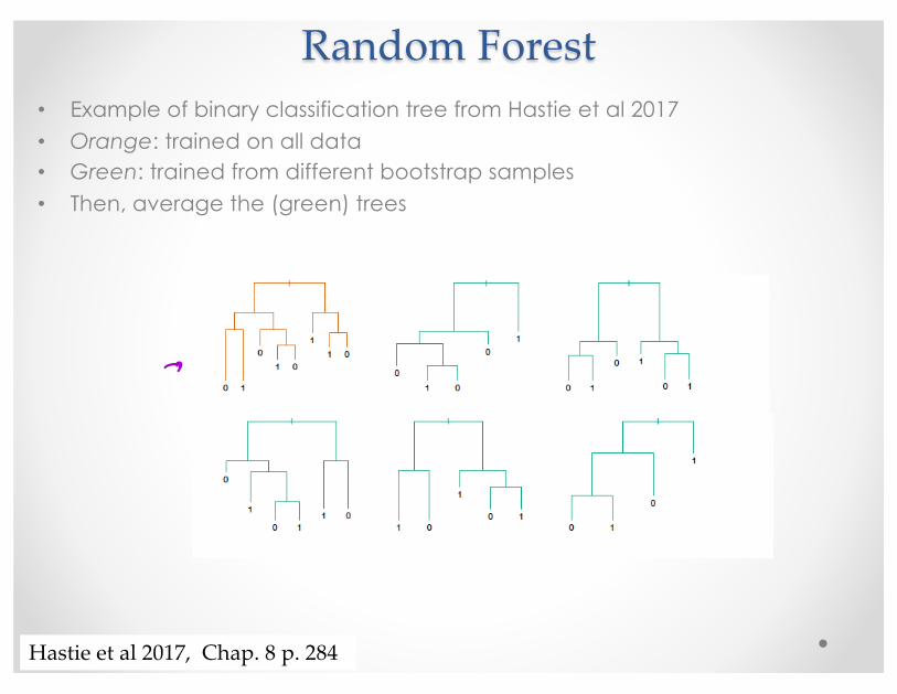
Random Forest• Example of binary classification tree from Hastie et al 2017• Orange: trained on all data• Green: trained from different bootstrap samples• Then, average the (green) trees
Example: baggingExample (from ESL 8.7.1): n = 30 training data points, p = 5features, and K = 2 classes. No pruning used in growing trees:
10
Example: baggingExample (from ESL 8.7.1): n = 30 training data points, p = 5features, and K = 2 classes. No pruning used in growing trees:
10Hastie et al 2017, Chap. 8 p. 284
Random Forest• Bootstrap + bagging => more robust RF on future test data• Train each tree Tb on bootstrap sampling
Hastie et al 2017, Chap. 15 p. 588
T
Timeseries (TS)• Timeseries: one or more variables sampled in the same location at successive time steps
ARMA• Autoregressive moving-average :
o (weakly) stationary stochastic processo Polynomials model process and errors as polynomial of prior values
• Autogressive (order p)o Linear model of past (lagged) and future valueso p lags
o φi are (weights) parameterso c is constanto εt is white noise (WGN)o Note, for stationary processes, |φi|< 1.
• Moving-average (order q)o Linear model of past errorso q lagso Below, assume <Xt>=0 (expectation is 0)
Xt = c+ ϕi X t−i +εti=1
p
∑
Xt = c+ θiεt−i +εti=1
q
∑
O
T
ARMA• Autoregressive moving-average :
o (weakly) stationary stochastic processo Linear model of prior values = expected value term + error term + WGN
• ARMA: AR(p) + MA(q)
Xt = c+ ϕi X t−i +i=1
p
∑ θiεt−i +εti=1
q
∑
Data retrievalJust a few public data sources for physical sciences…
• NOAA:o Reanalysis/model data, research cruises, station observations, gridded data products,
atmospheric & ocean indices timeseries, heat budgets, satellite imagery• NASA:
o EOSDIS, gridded data products (atmospheric), satellite imagery, reanalysis/model data, meteorological stations, DAAC’s in US
• IMOS: o ocean observing hosted by Australian Ocean Data Network
• USGS Earthquake Archives• CPC/NCEI:
o gridded and raw meteorological and oceanographic• ECMWF
o global-scale weather forecasts and assimilated data…
Possible data formats:o CSVo NetCDFo HDF5/HDF-EOSo Binaryo JPEG/PNGo ASCII text
……
Basic data cleaning
• “[ML for physical sciences] is 80% cleaning and 20% models” ~ paraphrased, Dr. Gerstoft• Basic cleaning for NOAA GSOD to HW – necessary
o Remove unwanted variables (big data is slow)o Replaced “9999” filler values with NaNo Converted strings to floats (i.e. for wind speed)o Created a DateTime index
• Physical data needs cleaning, reorganizing• Quality-controlled data still causes bugs• Application-specific
r
r
n
Data for HW• BigQuery:
o Open-source database hosted by Google o Must have Google accounto 1 TB data free/ month NOAA GSOD dataset
f
Data for HW• How to get BigQuery data?• bigquery package in Jupyter Notebook (SQL server)
• More complex queries may include dataframe joins, aggregations, or subsetting
Yearly datasets Simple SQL query
Query client and convert to Pandas DF
Pickle the DF
ii
k
Tutorial Notebook
• Open “In-Class Tutorial”• We will do:
1. Load preprocessed data2. Define timeseries index3. Look at data4. Visualize station5. Detrend data6. Smooth data7. Try ARMA model
Tutorial Notebook• Load packages, (pre-processed) data with Pandas
import packages
load data
find where data is after 2008
Timeseries processing• We may be missing data, but that’s ok for now• Replace with neighbor data, smooth, fill with mean
missing data
O
Tutorial Notebook
Basemap is handy but some problems if running on your laptop
n
O
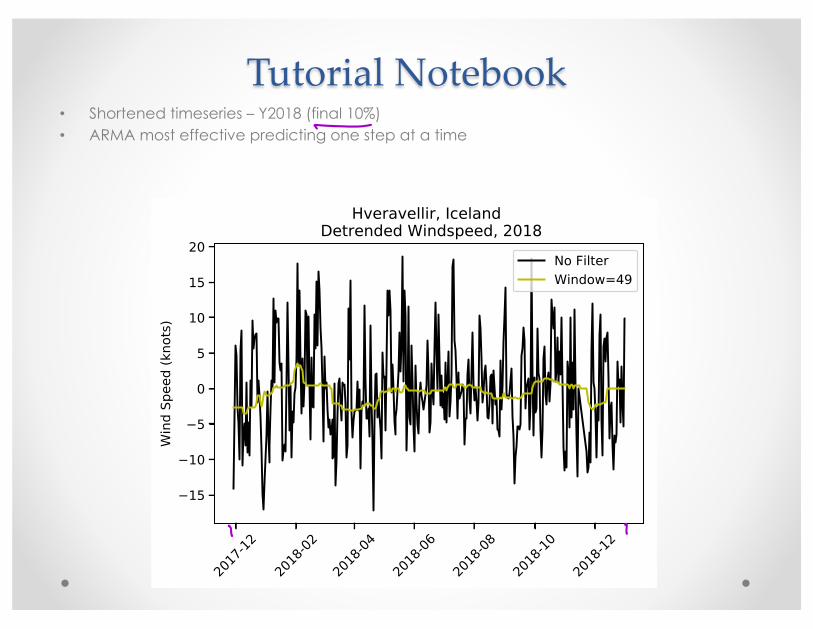
Timeseries processing• Remove mean (slope=0) or linear (slope ≠ 0)? (linear)• What can we learn from trend?
Timeseries processing• Smoothing: median filter
Tutorial Notebook• Shortened timeseries – Y2018 (final 10%)• ARMA most effective predicting one step at a time
I 7
Tutorial Notebook• Is ARMA a machine learning technique? (I think so..)
o Filtering method (like Kalman filter)o Data-driveno Maximum likelihoodo Conclusion: statistics-based
Tutorial Notebook• Autocorrelation:
o A statistical method to find temporal (or spatial) relations in datao When can reject the null hypothesis that the data is statistically similar?o E.g. How many time steps before the data is decorrelated
~40 lags
I
9
T
Tutorial Notebook• Median filter increases decorrelation scale
o By averaging neighbor samples• Raw series is more random• Use raw timeseries
~3 lags
Tutorial Notebook• ARMA algorithm:
1. Train on all previous data2. Predict one time step3. Add next value to training data4. Repeat
Homework• How to load and preview data with Pandas
import packages
load data
find where data is after 2008
Homework• How to load and preview data with Pandas
column of all temperature
entries
corresponding recording
station
Homework• Randomly select a station• Check if the station has enough data
o May reduce “3650” to lower number, i.e. 1000, but be aware you may have nans in data – just look at it!
Homework• (Map is supposed to show red “X” for station)
I can barely see it!!
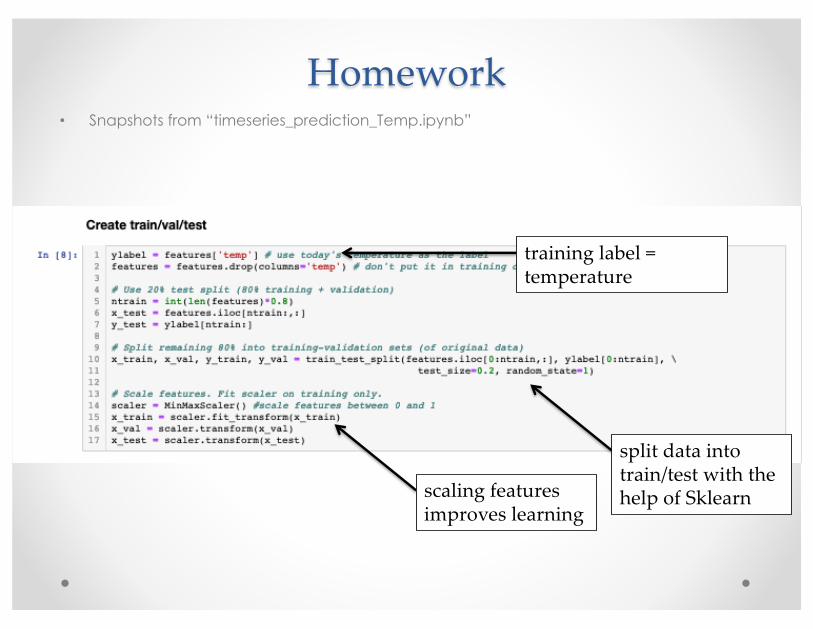
Homework• Snapshots from “timeseries_prediction_Temp.ipynb”
training label = temperature
split data into train/test with the help of Sklearnscaling features
improves learning
Homework• Random forest model in a couple lines• You may want to write a “plot.py” function
Define, train, and predict with random forest
plotting true and predicted temperature
look at feature importances
Homework• Congratulations!• We showed that tomorrow’s temperature is usually similar to today’s (at this Canada
station)
unsurprising result:validates intuition
Fei-Fei Li & Justin Johnson & Serena Yeung Lecture 7 - April 25, 2017Fei-Fei Li & Justin Johnson & Serena Yeung Lecture 7 - April 25, 201797
Takeaway for your projects and beyond:Have some dataset of interest but it has < ~1M images?
1. Find a very large dataset that has similar data, train a big ConvNet there
2. Transfer learn to your dataset
Deep learning frameworks provide a “Model Zoo” of pretrained models so you don’t need to train your ownCaffe: https://github.com/BVLC/caffe/wiki/Model-ZooTensorFlow: https://github.com/tensorflow/modelsPyTorch: https://github.com/pytorch/vision