37
Homoclinic Bifurcations to Equilibria II. Numerical continuation Alan Champneys University of Bristol Department of Engineering Mathematics MRI Master Class Utrecht – p. 1
| Date post: | 08-Mar-2018 |
| Category: |
Documents |
| Upload: | truongdang |
| View: | 216 times |
| Download: | 0 times |
Homoclinic Bifurcations toEquilibria
II. Numerical continuation
Alan Champneys University of Bristol
Department of Engineering Mathematics
MRI Master Class Utrecht – p. 1

Outline: Lecture 2
1. HomCont: continuation of homoclinic orbits in AUTOprojection boundary conditions for homoclinicsheteroclinic orbits4 ways startconservative systems
2. Codimension-two homoclinic bifurcationseigenvalue degeneraciesnon-hyperbolic equilibriaorientation flipsother cases
3. HomCont implementation of codim-2 cases
MRI Master Class Utrecht – p. 2

Homoclinic orbit continuation
C. Kuznetsov, Sandstede 95Consider the BVP on an infinite interval
x(t) = f(x(t), α), x ∈ Rn, α ∈ R
p, f ∈ Cr
f(x0, α) = 0,
x(t) → x0 as t→ ±∞.
Plus phase condition∫ ∞−∞
˙xT(t)[x(t) − x(t)]dt = 0 whichminimises L2 distance from reference solution x (previoussolution on branch).Well posed provided equilibrium x0(α) is hyperbolic:
A := Dxf(x0, α) has ns stable and nu unstable eigs:ns + nu = n.
MRI Master Class Utrecht – p. 3
Basic idea
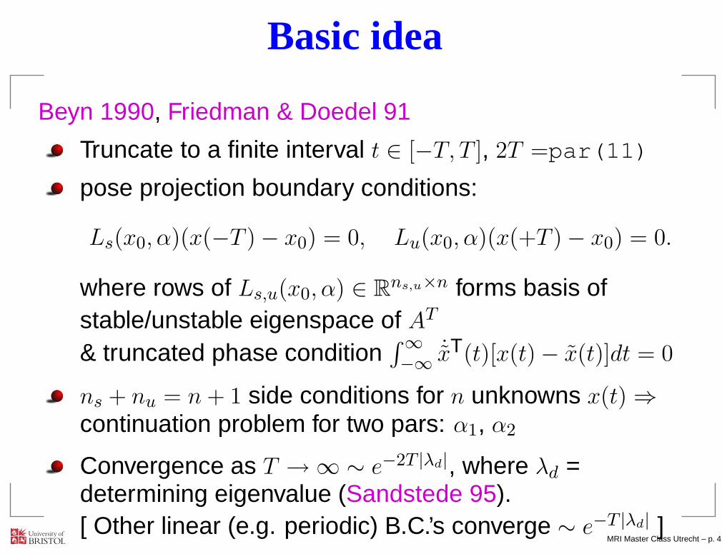
Beyn 1990, Friedman & Doedel 91
Truncate to a finite interval t ∈ [−T, T ], 2T =par(11)
pose projection boundary conditions:
Ls(x0, α)(x(−T ) − x0) = 0, Lu(x0, α)(x(+T ) − x0) = 0.
where rows of Ls,u(x0, α) ∈ Rns,u×n forms basis of
stable/unstable eigenspace of AT
& truncated phase condition∫ ∞−∞
˙xT(t)[x(t) − x(t)]dt = 0
ns + nu = n+ 1 side conditions for n unknowns x(t) ⇒continuation problem for two pars: α1, α2
Convergence as T → ∞ ∼ e−2T |λd|, where λd =determining eigenvalue (Sandstede 95).[ Other linear (e.g. periodic) B.C.’s converge ∼ e−T |λd| ]
MRI Master Class Utrecht – p. 4
Heteroclinic case
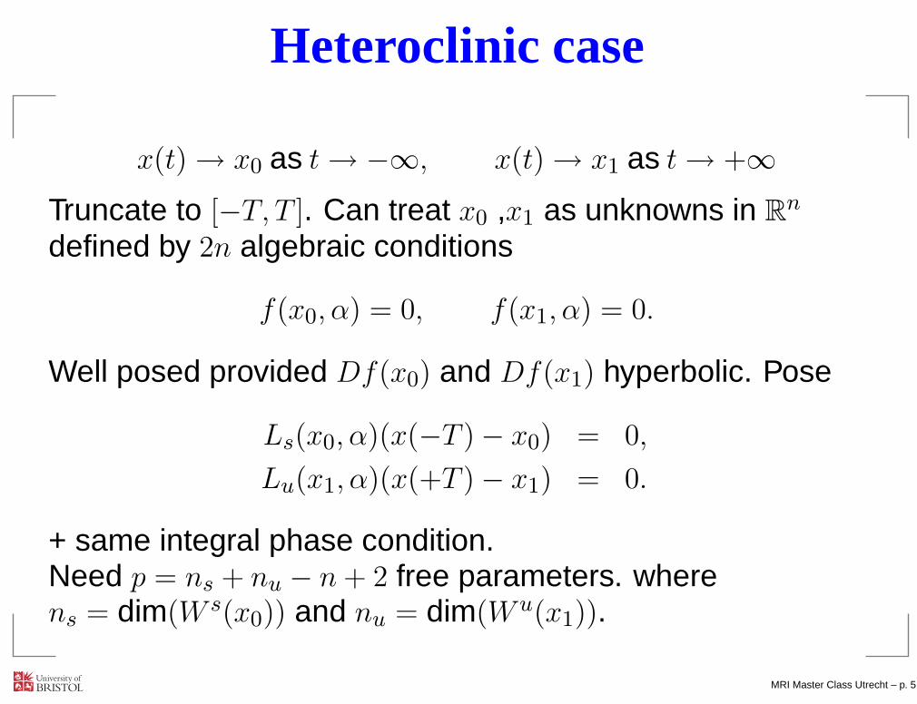
x(t) → x0 as t→ −∞, x(t) → x1 as t→ +∞
Truncate to [−T, T ]. Can treat x0 ,x1 as unknowns in Rn
defined by 2n algebraic conditions
f(x0, α) = 0, f(x1, α) = 0.
Well posed provided Df(x0) and Df(x1) hyperbolic. Pose
Ls(x0, α)(x(−T ) − x0) = 0,
Lu(x1, α)(x(+T ) − x1) = 0.
+ same integral phase condition.Need p = ns + nu − n+ 2 free parameters. wherens = dim(W s(x0)) and nu = dim(W u(x1)).
MRI Master Class Utrecht – p. 5
AUTO implementation
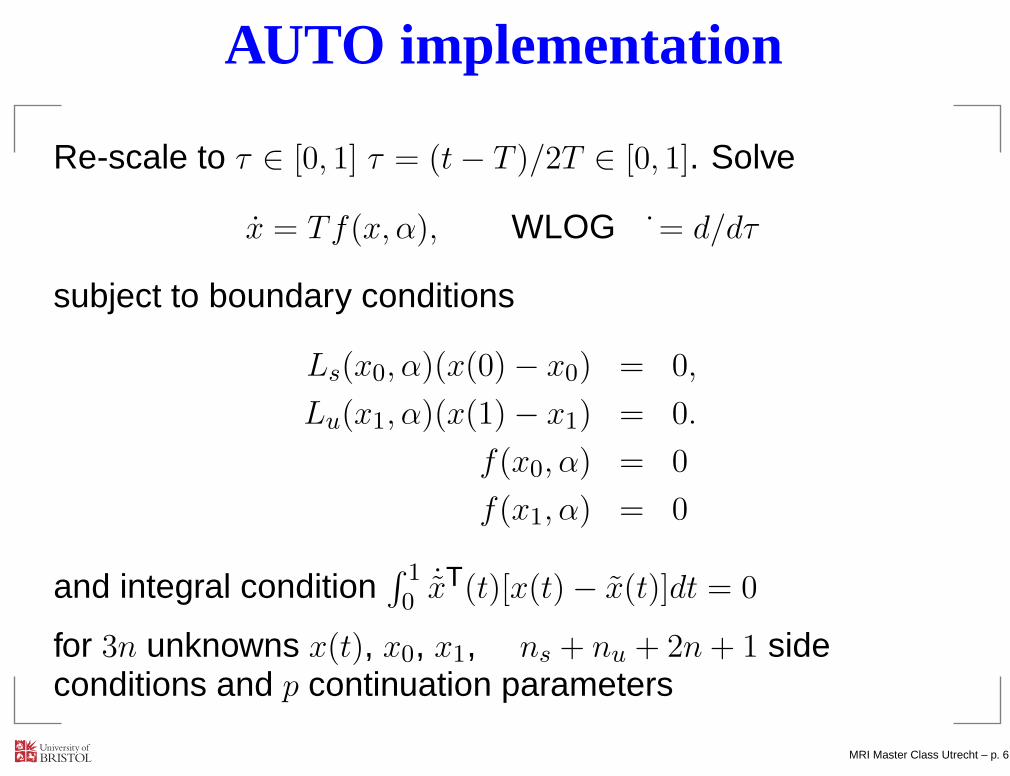
Re-scale to τ ∈ [0, 1] τ = (t− T )/2T ∈ [0, 1]. Solve
x = Tf(x, α), WLOG ˙= d/dτ
subject to boundary conditions
Ls(x0, α)(x(0) − x0) = 0,
Lu(x1, α)(x(1) − x1) = 0.
f(x0, α) = 0
f(x1, α) = 0
and integral condition∫ 10
˙xT(t)[x(t) − x(t)]dt = 0
for 3n unknowns x(t), x0, x1, ns + nu + 2n+ 1 sideconditions and p continuation parameters
MRI Master Class Utrecht – p. 6
HomCont
AUTO sets up these boundary conditions (and rescalingto τ ∈ [0, 1]) automatically
User should specify ns=NSTAB, nu= NUNSTAB, andIEQUIB = 0 or -1 for explicit equilibria OR IEQUIB= 1 or -2 for continued equilibria
Actually NSTAB and NUNSTAB can be automaticallydetected using eigenvalues of Df(x0) in homocliniccase.
Several ways to start, using ISTART . . .
MRI Master Class Utrecht – p. 7
Ways to start
ISTART=1 Data from a previous numerical integration is readinto AUTO using the @fc command. This data shouldbe in multicolumn format T, [U(i), i = 1 . . . n]. Seee.g. demo cir.
ISTART=2 An explicit homoclinic solution is stored in STPNT.See e.g. demo san.
ISTART=3 The “homotopy method” . . . see e.g. demo kpr
ISTART=4 Data from a large-period periodic orbit. AUTO firstperforms a computation to “rotate” the data so that theequilibrium is at τ = 0 and τ = 1.
MRI Master Class Utrecht – p. 8
Starting using homotopy
(for homoclinic case with real eigenvalues λi, eigenvects vi)
Start with small solution tangent to W u(x0):
x(0) = x0 + ǫ0
nu∑
i=1
ξivieλiTτ , T ≪ 1,
nu∑
i=1
ξ2i = 1
Continue in T = PAR(11), and one ξi. monitor testfunctions ωi = wT
i (x(1) − x(0)), i = 1, . . . nu whereDfTwi = λiwi.
Freeze T , successively free up ξi and α to look for zerosof ωj = 0.
Continue in T again, freeing up a parameter butfreezing all ωi = 0 until x(1) − x0 = O(ǫ0)
Recommend to use only in case nu = 1. MRI Master Class Utrecht – p. 9

Conservative case
(including Hamiltonian)
Suppose x = f(x, α) conserves a integral H(x, α).
Then homoclinic orbits are codim 0, since W u(x0) andW s(x0) are contained in level set H(x) = const.
Use the conserved quantity H = const. to include adummy free parameter,
x = f(x, α) + α0∇H(x)
and use regular algorithm to continue in two freeparameters α1, α0 where α1 is a regular problemparameter. True solution has α0 = 0 ⇒ accuracy test.
See Doedel’s lectures for extensions . . .
MRI Master Class Utrecht – p. 10
2. Codim 2 homoclinic bifurcations
Interesting as ‘organising centres’ for parameter space;birth of multi-pulse homoclinics etc.sources of degeneracy in codim 1 bifurcation:
eigenvalue degeneracy (hyperbolic cases)
non-hyperbolic equilibrium (saddle-node, Hopf)
(for real saddle) orientable → twisted transition
other cases
MRI Master Class Utrecht – p. 11
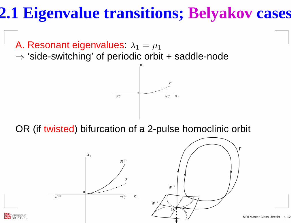
2.1 Eigenvalue transitions;Belyakovcases
A. Resonant eigenvalues: λ1 = µ1
⇒ ‘side-switching’ of periodic orbit + saddle-node
0(1)1
2
1α2(1)
(1)S
H H
α
OR (if twisted) bifurcation of a 2-pulse homoclinic orbit
0(1)1
2
(2)
F
(1)2 1H
H
H α
α
O
Γ
W
W u
s
MRI Master Class Utrecht – p. 12
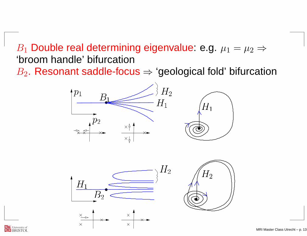
B1 Double real determining eigenvalue: e.g. µ1 = µ2 ⇒‘broom handle’ bifurcationB2. Resonant saddle-focus ⇒ ‘geological fold’ bifurcationp1 p2B1 H1H2 H1
H2H2H1 B2MRI Master Class Utrecht – p. 13
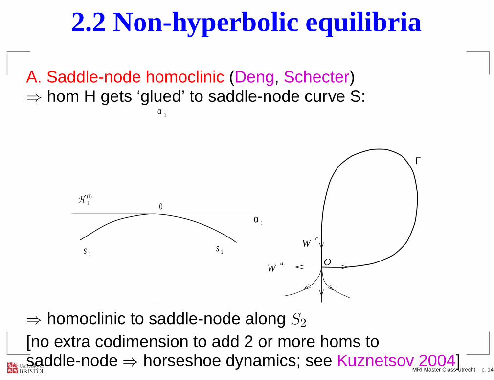
2.2 Non-hyperbolic equilibria
A. Saddle-node homoclinic (Deng, Schecter)⇒ hom H gets ‘glued’ to saddle-node curve S:
0
s
(1)1
α
1 2
1
H
2
s
α
OW
u
Wc
Γ
⇒ homoclinic to saddle-node along S2
[no extra codimension to add 2 or more homs tosaddle-node ⇒ horseshoe dynamics; see Kuznetsov 2004]
MRI Master Class Utrecht – p. 14
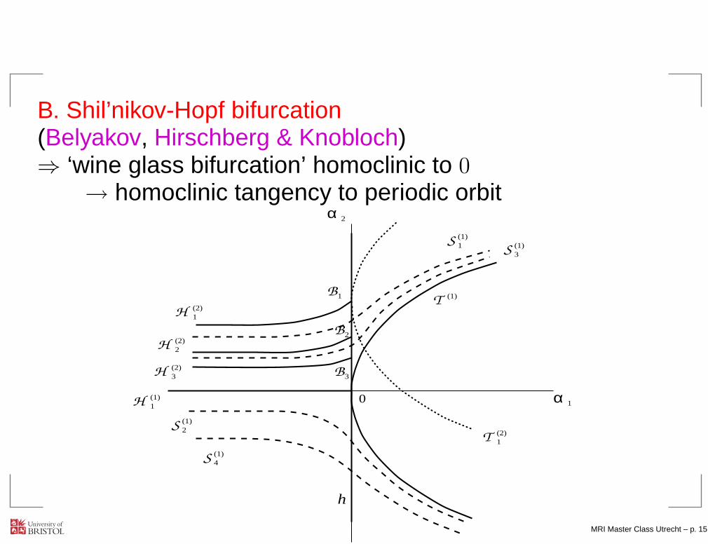
B. Shil’nikov-Hopf bifurcation(Belyakov, Hirschberg & Knobloch)⇒ ‘wine glass bifurcation’ homoclinic to 0
→ homoclinic tangency to periodic orbit
0
α
T
h
2
1
(2)1
(2)2
(2)3
(1)1
α(1)2
(1)4
1
2
3
(1)1 (1)
3
(1)
(2)1
H
H
H
H
S
S
B
B
B
SS
T
MRI Master Class Utrecht – p. 15
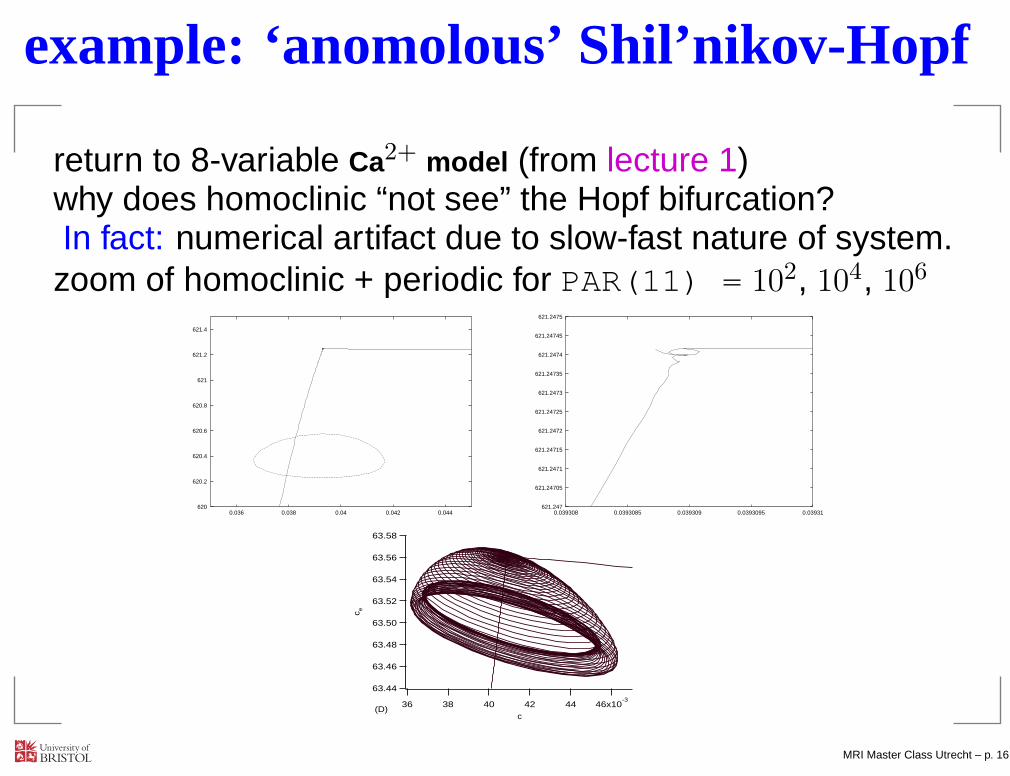
example: ‘anomolous’ Shil’nikov-Hopf
return to 8-variable Ca2+ model (from lecture 1)why does homoclinic “not see” the Hopf bifurcation?In fact: numerical artifact due to slow-fast nature of system.zoom of homoclinic + periodic for PAR(11) = 102, 104, 106
620
620.2
620.4
620.6
620.8
621
621.2
621.4
0.036 0.038 0.04 0.042 0.044621.247
621.24705
621.2471
621.24715
621.2472
621.24725
621.2473
621.24735
621.2474
621.24745
621.2475
0.039308 0.0393085 0.039309 0.0393095 0.03931
63.58
63.56
63.54
63.52
63.50
63.48
63.46
63.44
c e
46x10-3
4442403836
c(D)
MRI Master Class Utrecht – p. 16
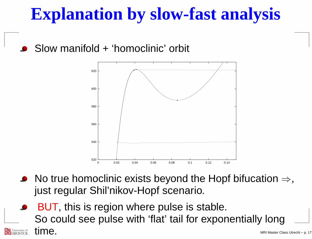
Explanation by slow-fast analysis
Slow manifold + ‘homoclinic’ orbit
520
540
560
580
600
620
0 0.02 0.04 0.06 0.08 0.1 0.12 0.14
No true homoclinic exists beyond the Hopf bifucation ⇒,just regular Shil’nikov-Hopf scenario.
BUT, this is region where pulse is stable.So could see pulse with ‘flat’ tail for exponentially longtime. MRI Master Class Utrecht – p. 17
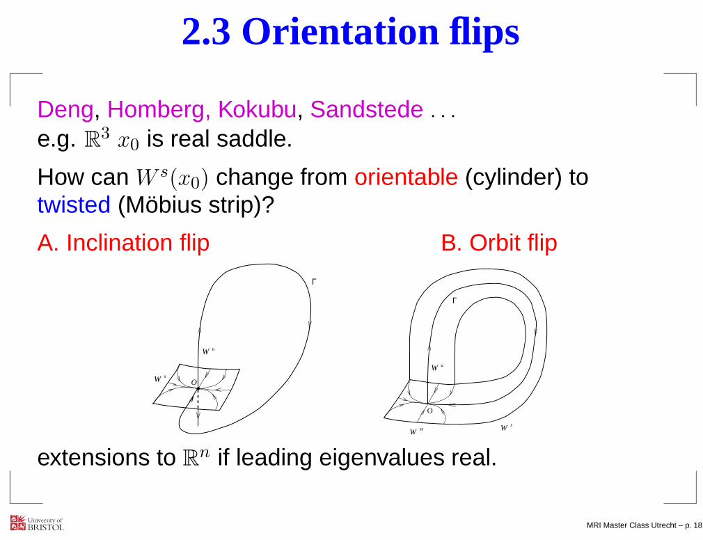
2.3 Orientation flips
Deng, Homberg, Kokubu, Sandstede . . .e.g. R
3 x0 is real saddle.
How can W s(x0) change from orientable (cylinder) totwisted (Möbius strip)?
A. Inclination flip B. Orbit flip
O
W
Γ
W s
u
s
O
W W
W
Γ
u
ss
extensions to Rn if leading eigenvalues real.
MRI Master Class Utrecht – p. 18
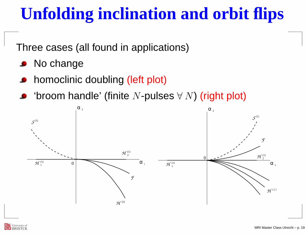
Unfolding inclination and orbit flips
Three cases (all found in applications)
No change
homoclinic doubling (left plot)
‘broom handle’ (finite N -pulses ∀N ) (right plot)
10
F
(1)
2
(1)
α
2
(2)
(1)1
S
H
H
H
α0
F
(1)1
2
H
(1)
(1)2
1
( j )
H
S
H
α
α
MRI Master Class Utrecht – p. 19
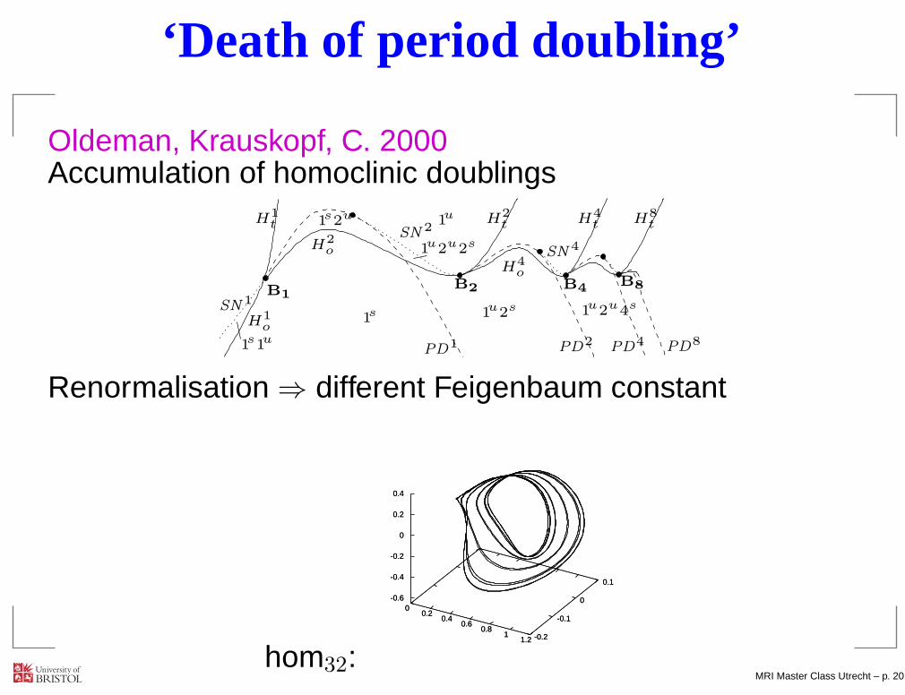
‘Death of period doubling’
Oldeman, Krauskopf, C. 2000Accumulation of homoclinic doublings
B1
SN2
SN1
H2
o
H4
o
SN4
B2 B4B8
1s 1
u2
s
1u2
u2
s
1s2
u
H1
o
1u2
u4
s
PD1 PD
2PD
8PD
4
1u
1s1u
H2
tH1
tH4
tH8
t
Renormalisation ⇒ different Feigenbaum constant
hom32:
00.2
0.40.6
0.81
1.2 -0.2
-0.1
0
0.1
-0.6
-0.4
-0.2
0
0.2
0.4
00.2
0.40.6
0.81
1.2 -0.2
-0.1
0
0.1
-0.6
-0.4
-0.2
0
0.2
0.4
MRI Master Class Utrecht – p. 20
2.4 Other kinds of codimension-two homoclinics
Not covered in these lectures
Local birth of homoclinic orbits e.g.from Takens-Bogdanov (implemented in MatCont!)or Saddle-node Hopf (see e.g. C. & Kirk 2004)
Forming heteroclinic cycle with other equilibrium(T -points)
Forming a heteroclinic cycle with a periodic orbit (seee.g. C., Kirk et al 2009)
. . .
MRI Master Class Utrecht – p. 21
3. Codim 2 homoclinics in HomCont
Concept: find a test function ψ(x(t), α)
Defined and smooth in a neighbourhood of the truecurve of codim 1 homoclinic orbits H in function andparameter space.
Has a regular zero in theory at the codim 2 point inquestion
Has a regular zero for the truncated problem HT forsufficiently large T > 0
its zero tends to the true one as T → ∞
can append ψ = 0 to continuation problem to continuecodim 2 points in three pars.
MRI Master Class Utrecht – p. 22
3.1 Eigenvalue degeneracies
Compute eigenvalues of A(x0, α) = Dxf(x0, α) and orderaccording to real part.
Negative real part: µi, i = 1, 2, . . . , ns
zero real part: γj , j = 1, 2, . . . , n0
positive real part: λk, k = 1, 2, . . . , nu
Re µns≤ · · · ≤ Re µ1 < 0 < Re λ1 ≤ · · · ≤ Re λnu
.
MRI Master Class Utrecht – p. 23
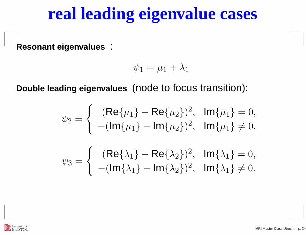
real leading eigenvalue cases
Resonant eigenvalues :
ψ1 = µ1 + λ1
Double leading eigenvalues (node to focus transition):
ψ2 =
{
(Re{µ1} − Re{µ2})2, Im{µ1} = 0,
−(Im{µ1} − Im{µ2})2, Im{µ1} 6= 0.
ψ3 =
{
(Re{λ1} − Re{λ2})2, Im{λ1} = 0,
−(Im{λ1} − Im{λ2})2, Im{λ1} 6= 0.
MRI Master Class Utrecht – p. 24
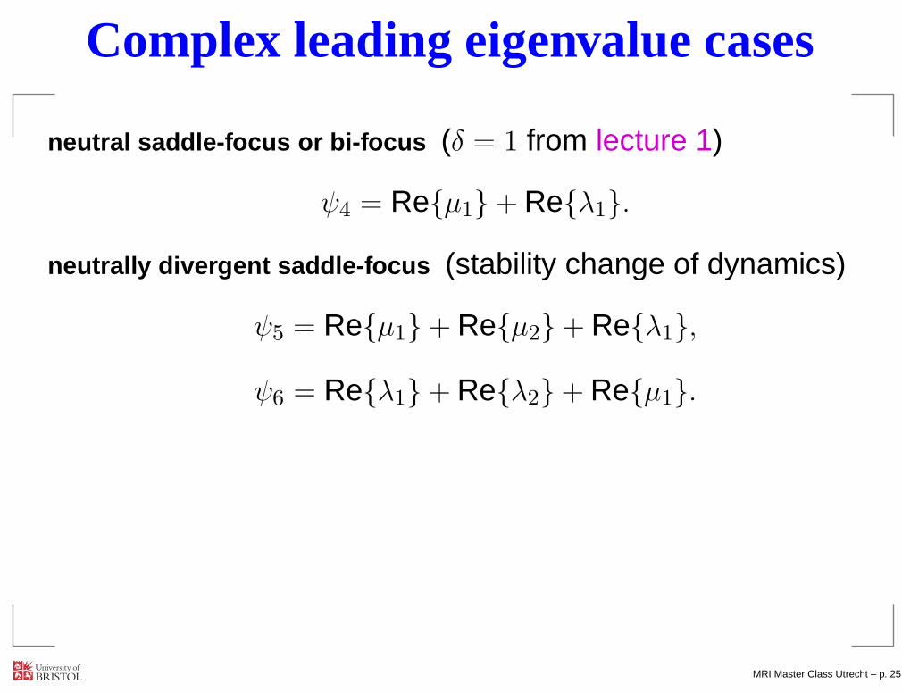
Complex leading eigenvalue cases
neutral saddle-focus or bi-focus (δ = 1 from lecture 1)
ψ4 = Re{µ1} + Re{λ1}.
neutrally divergent saddle-focus (stability change of dynamics)
ψ5 = Re{µ1} + Re{µ2} + Re{λ1},
ψ6 = Re{λ1} + Re{λ2} + Re{µ1}.
MRI Master Class Utrecht – p. 25
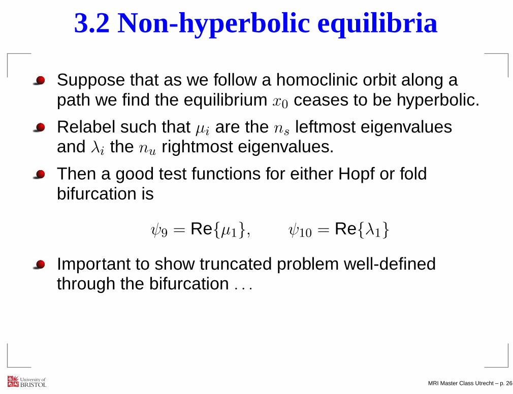
3.2 Non-hyperbolic equilibria
Suppose that as we follow a homoclinic orbit along apath we find the equilibrium x0 ceases to be hyperbolic.
Relabel such that µi are the ns leftmost eigenvaluesand λi the nu rightmost eigenvalues.
Then a good test functions for either Hopf or foldbifurcation is
ψ9 = Re{µ1}, ψ10 = Re{λ1}
Important to show truncated problem well-definedthrough the bifurcation . . .
MRI Master Class Utrecht – p. 26

Shil’nikov-Hopf bifurcation
H
x∗
W s(x∗)
H(1) H(1)
Γ1
Γ
x∗
x∗
Γ0
α1
0 :
0
H(1) : H(1) :
α2
W s(C)C
Numerical problem approximates H(1) ∪ H(1):H(1) is curve of homoclinicsH(1) is curve of point-periodic connections
MRI Master Class Utrecht – p. 27
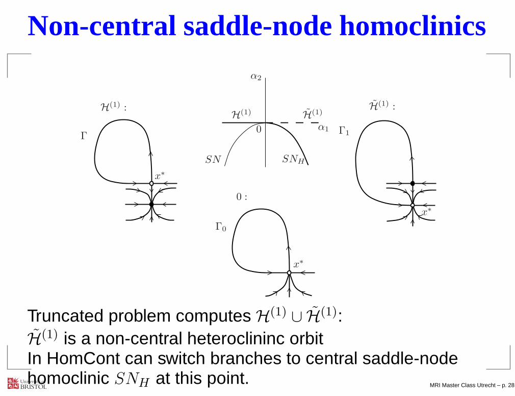
Non-central saddle-node homoclinics
SN SNH
H(1) H(1)
α1
α2
0 :
H(1) : H(1) :
0
x∗
Γ
x∗
Γ0
Γ1
x∗
Truncated problem computes H(1) ∪ H(1):H(1) is a non-central heteroclininc orbitIn HomCont can switch branches to central saddle-nodehomoclinic SNH at this point. MRI Master Class Utrecht – p. 28

Continuation of saddle-node homoclinics
(central case - tangent to centre eigenspace as t→ ±∞)
Consider equilibrium x0 precisely at fold point with 1Dcentre manifold: nc = 1, nu + ns = n− 1
At fold point homoclinic is in intersection of W cs andW cu ⇒ no extra codimension.
The usual projection B.C.’s now give n− 1 equations
Ls(x0, α)(x(0) − x0) = 0, Lu(x0, α)(x(1) − x0) = 0.
+ phase condition, but need constraint to stay on foldcurve:
detA(x0, α) = 0
MRI Master Class Utrecht – p. 29
3.3. Orientation flips
Suppose leading eigenvalues are real µ1 < 0 < λ1
let ws1(α) and wu
1 (α) be normalised adjoint eigenvectors
AT(x0, α)ws1 = µ1w
s1 AT(x0, α)wu
1 = λ1wu1 .
which are chosen to depend smoothly on α
similarly let vs1(α) and vu
1 (α) be normalised eigenvectors
A(x0, α) vs1 = µ1 v
s1 A(x0, α) vu
1 = λ1 vu1 .
chosen to vary smoothly with α
MRI Master Class Utrecht – p. 30
Orbit flip
Generically homoclinic orbit x(t) − x0 ≈ Kv1eµt as
t→ ∞. Where
K = limt→∞
e−µ1t 〈ws1, x(t) − x0〉
Orbit flip w.r.t. W s occurs if K = 0 at codim two point.
Similarly, orbit flip w.r.t. W u occurs if
limt→−∞
eλ1t 〈wu1 , x(t) − x0〉 = 0
Therefore test functions for orbit flip:
ψ11 = e−µ1T 〈ws1, x(+T ) − x0〉
ψ12 = eλ1T 〈wu1 , x(−T ) − x0〉
MRI Master Class Utrecht – p. 31
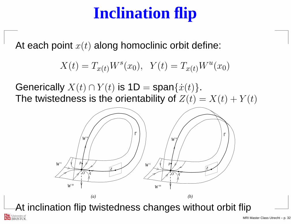
Inclination flip
At each point x(t) along homoclinic orbit define:
X(t) = Tx(t)Ws(x0), Y (t) = Tx(t)W
u(x0)
Generically X(t) ∩ Y (t) is 1D = span{x(t)}.The twistedness is the orientability of Z(t) = X(t) + Y (t)
Z Z
Γ
W
W
s
u
O
W
W
s
u
O
W Wss ss
p
q q
p
(a) (b)
Γ
At inclination flip twistedness changes without orbit flipMRI Master Class Utrecht – p. 32
Consider adjoint variational problem:
ϕ = −(Dxf)T(x(t), α)ϕ,
Nondegenerate homoclinic ⇒ unique (up to scale)bounded solution ϕ(t) → 0 as t→ ±∞
ϕ(t) is normal vector to Z(t).
Generically, ϕ(t) ≈ Kws1e
−µ1t as t→ ∞, where
K = limt→−∞
eµ1t 〈vs1, ϕ(t)〉
Inclination flip w.r.t. stable manifold occurs when K = 0at codim 2 point along homoclinic branch.
MRI Master Class Utrecht – p. 33
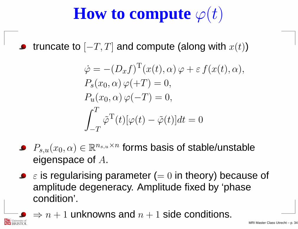
How to computeϕ(t)
truncate to [−T, T ] and compute (along with x(t))
ϕ = −(Dxf)T(x(t), α)ϕ+ ε f(x(t), α),
Ps(x0, α)ϕ(+T ) = 0,
Pu(x0, α)ϕ(−T ) = 0,∫ T
−T
ϕT(t)[ϕ(t) − ϕ(t)]dt = 0
Ps,u(x0, α) ∈ Rns,u×n forms basis of stable/unstable
eigenspace of A.
ε is regularising parameter (= 0 in theory) because ofamplitude degeneracy. Amplitude fixed by ‘phasecondition’.
⇒ n+ 1 unknowns and n+ 1 side conditions.MRI Master Class Utrecht – p. 34
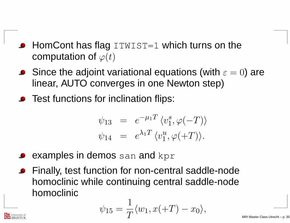
HomCont has flag ITWIST=1 which turns on thecomputation of ϕ(t)
Since the adjoint variational equations (with ε = 0) arelinear, AUTO converges in one Newton step)
Test functions for inclination flips:
ψ13 = e−µ1T 〈vs1, ϕ(−T )〉
ψ14 = eλ1T 〈vu1 , ϕ(+T )〉.
examples in demos san and kpr
Finally, test function for non-central saddle-nodehomoclinic while continuing central saddle-nodehomoclinic
ψ15 =1
T〈w1, x(+T ) − x0〉,
MRI Master Class Utrecht – p. 35
What we have learnt
How to continue homo/heteroclinic orbits directly inAUTO
Special cases for homoclinics to saddle-node equilibria
Certain kinds of codimension-two homoclinic orbits
How to detect and continue them in AUTO usingHomCont
Important in applications for tame to chaotic transitionsand bifurcation of multi-pulses.
MRI Master Class Utrecht – p. 36
References
Beyn, W.-J. The numerical computation of connecting orbits in dynamical systems,IMA J. Numerical Analysis 9 (1990) 379-405.
Champneys, A.R. Kirk, V. Knobloch, E. Oldeman, B.E. and Sneyd, J. When Shil’nikovmeets Hopf in excitable systems, SIAM J. Appl. Dyn. Syst., 6 (2007) 663-693.
Champneys, A.R. and Kuznetsov, Yu.A., Numerical detection and continuation ofcodimension-two homoclinic bifurcations, Int. J. Bifurcation & Chaos 4 (1994) 795-822.
Champneys, A.R. Kuznetsov, Yu.A. and Sandstede, B. A numerical toolbox forhomoclinic bifurcation analysis, Int. J. Bifurcation & Chaos 6 (1996) 867-887.
Friedman, M.J. and Doedel, E.J. Numerical computation and continuation of invariantmanifolds connecting fixed points SIAM J. Num.. Anal., 28 (1991) 789-808.
Kuznetsov, Yu.A. Elements of Applied Bifurcation Theory (3rd Edn) Springer-Verlag(2004)
Sandstede, B. Convergence estimates for the numerical approximation of homoclinicsolutions IMA J. of Numerical Analysis 17 (1997) 437-462.
MRI Master Class Utrecht – p. 37


