RA Economics and institutional change

Homophily and Triadic Closure in Evolving Social Networks

Irene Crimaldi Michela Del Vicario Greg Morrison Walter Quattrociocchi Massimo Riccaboni

IMT LUCCA EIC WORKING PAPER SERIES 03

May 2015

#03 2015

IMT LUCCA EIC WORKING PAPER SERIES #03/2015 © IMT Institute for Advanced Studies Lucca

Piazza San Ponziano 6, 55100 Lucca

Research Area

Economics and institutional change

Homophily and Triadic Closure in Evolving Social Networks

Irene Crimaldi IMT Institute for Advanced Studies Lucca

Michela Del Vicario IMT Institute for Advanced Studies Lucca

Greg Morrison IMT Institute for Advanced Studies Lucca

Walter Quattrociocchi IMT Institute for Advanced Studies Lucca

Massimo Riccaboni IMT Institute for Advanced Studies Lucca

Homophily and Triadic Closure

in Evolving Social Networks

Irene Crimaldi, Michela Del Vicario, Greg Morrison,Walter Quattrociocchi, Massimo Riccaboni ∗

April 30, 2015

Abstract

We present a new network model accounting for homophily and triadic closure

in the evolution of social networks. In particular, in our model, each node ischaracterized by a number of features and the probability of a link betweentwo nodes depends on common features. The bipartite network of the actorsand features evolves according to a dynamics that depends on three parame-ters that respectively regulate the preferential attachment in the transmissionof the features to the nodes, the number of new features per node, and thepower-law behavior of the total number of observed features. We providetheoretical results and statistical estimators for the parameters of the model.We validate our approach by means of simulations and an empirical analysisof a network of scientific collaborations.

keyword: social network, bipartite network, preferential attachment, homophily,triadic closure, transitivity.

1 Introduction

Social networks are characterized by a number of general properties [5, 15, 18, 28,30, 58]. The issue that has recently received more attention is the distribution of thenumber of node’s connections, which is well approximated by a power-law in manycontexts. Preferential attachment is generally accepted as the simplest mechanismthat can reproduce such a distribution [2, 3]. This basic mechanism, however, is

∗Alphabetic order. IMT Institute for Advanced Studies Lucca, Piazza San Ponziano6, I-55100 Lucca, Italy. E-mail: irene.crimaldi@imtlucca.it, michela.delvicario@imtlucca.it(corresponding author), greg.morrison@imtlucca.it, walter.quattrociocchi@imtlucca.it and mas-simo.riccaboni@imtlucca.it. Irene Crimaldi is a member of the Italian Group “Gruppo Nazionaleper l’Analisi Matematica, la Probabilita e le loro Applicazioni (GNAMPA)” of the Italian Institute“Istituto Nazionale di Alta Matematica (INdAM)”.

1

only one of the many social forces that contribute to shape the evolution of socialnetworks. In particular, it is not able to reproduce the formation of social groups,or communities, and the composition of social circles.

Homophily, defined as the tendency of individuals to associate with others, simi-lar to them in some designed respect, is one of the most important mechanism thatguides social network evolution. A large body of research in sociology and, morerecently, in economics, confirms the prevalence of homophily in socio-economic net-works [38, 42]. Homophily, along the lines of race and ethnicity, age and sex, educa-tion, professional background and occupation, shapes social networks such as advice,marriage, exchange, communication, teamwork, co-membership, and friendship net-works [7, 8, 9, 14, 16, 19, 27, 31, 33, 34, 39, 40, 44, 50, 57]. Despite the multidi-mentional nature of homophily [11] is well recognized in the sociological literature,in formal models of network evolution it is typically represented by partitioningnodes into different classes. Indeed, some authors proposed to use conditional link-probabilities, given some (latent or observable) features, in such a way that thepresence of a common attribute induces a higher probability of a connection be-tween two nodes [1, 13, 20, 22, 23, 25, 32, 35, 47, 54]. These models, known asblock-models or cluster-models, assume that there exist some classes (also calledgroups, clusters, or types) to which a node can belong, but the assumption thateach node can belong only to a single class and/or the fact that the number ofclasses is finite and fixed a priori represent their main drawbacks.

Coming from a structural approach, network analysts have long debated thesources of network integration, using the concept of triadic closure, also called tran-sitivity or clustering [29, 48, 51]. Triadic closure is another strong candidate mecha-nism for the creation of links in social networks. This mechanism is at the basis ofmany generative network models [29, 55], and it is widely supported on the empiri-cal ground [18, 34, 45]. The triadic closure principle says that if A is a friend (i.e.neighbor) of B and B is a friend of C, then A and C have a high chance to becomefriends. Differently from homophily, such a process does not depend on the featuresof the nodes that get attached. Obviously, also homophily can naturally inducetriangles, but here, with the expression “triadic closure”, we refer to the formationof a link between two nodes by means of a common friend.

Recently, both mechanisms of network formation have been explicitly introducedin formal models of network evolution. However, most of the theoretical models sofar have been focusing on either homophily [16, 17, 43, 49, 52] or triadic closure[10, 24, 26, 41, 53, 56]. Against this background, we contribute to this growingbody of literature by introducing a new model accounting for both multidimen-sional homophily and triadic closure. More precisely, in our model, each node showsa number of features (the surrounding context, e.g. [18]), that can be of differentkinds (likings, inclinations, profile, spatial/geographical contexts, etc.), and differ-

2

ent nodes can share the same features. Differently from the above quoted works, weallow the number of features to grow in time. On its arrival, each new node linksto some nodes already present in the system. Firstly, the new node selects some“friends” (i.e. neighbors) according to probabilities that depend on the number ofcommon features (homophily). Then additional links can be established by means ofcommon friends, inducing the closure of some triplets (triadic closure). Our modelalso has the merit to provide a dynamics for the evolution of the features. Indeed,the bipartite nodes-features network evolves according to a model that depends onthree parameters that respectively regulate the preferential attachment in the trans-mission of the features to the nodes, the number of new features per node, and thepower-law behavior of the total number of observed features.

The present paper can be considered as a completion of [12]. Indeed, both ofthem provide a network model where link-probabilities are based on the nodes’ fea-tures, but they also show some differences. The main issue is that here we introducea parameter that tunes the preferential attachment in the transmission of the fea-tures to the nodes; while in [12] authors only consider a preferential attachment rule.However, in that paper a random “fitness” parameter which determines the node’sability to transmit its own features to other nodes (see also [6]) is attached to eachnode; while here we do not take into account fitness parameters for nodes.

The paper is structured as follows. In Section 2 we describe the basic assumptionsof our model and the notation used throughout the paper. In Section 3 we presentour model, that involves a dynamics for the bipartite network of nodes-featuresand the mechanism underlying the formation of the unipartite (i.e. node-node)network. In Section 4 we illustrate some theoretical results and we carefully explainthe meaning of each parameter inside our model. In Section 5 we show and discusssome statistical tools in order to estimate the model parameters from the data. InSection 6 we provide a number of simulations in order to point out the functioningof the model parameters and the ability of the proposed estimation tools. Section 7deals with an application of our model and instruments to a co-authorship network.The understanding of homophily and triadic closure in co-authorship networks isvery important since these two phenomena can affect the diffusion process of ideasand discoveries inside a certain research field and among different research fields[4, 21, 46]. Finally, in Section 8 we give our conclusions and discuss some futuredevelopments. The paper is enriched by an Appendix that contains a theorem andits proof, and supplementary simulation results.

2 Preliminaries

We assume new nodes sequentially joining the network so that node i represents theone that comes into the network at time step i.

3

Each node shows a finite number of features (the surrounding context, e.g. [18]),that can be of different kinds (likings, inclinations, profile, spatial/geographical con-texts, etc.), and different nodes can share the same features. It is worthwhile to notethat we do not specify a priori the total number of possible features. On its arrival,each new node links to some nodes already present in the system. Firstly, the newnode selects some “friends” (i.e. neighbors) according to probabilities that dependon the number of common features. This fact is in agreement with the principle,known as homophily, according to which individuals tend to be friends of peoplesimilar to themselves. Then additional links can be established by means of com-mon friends, inducing the closure of some triplets (triadic closure). It is worthwhileto note that also homophily can naturally induce triangles, but here, with the ex-pression “triadic closure”, we refer to the formation of a link between two nodesby means of a common friend. We postulate that the connections are undirectedand non-breakable and we omit self-loops (i.e. edges of type (i, i)). We denote theadjacency matrix (symmetric by assumption) by A, so that Ai,j = 1 when thereexists a link between nodes i and j, Ai,j = 0 otherwise. We set

Vj(i) = {j′ = 1, . . . , i : Aj,j′ = 1}

to be the set of node j’s neighbors at time step i (after the arrival of i).We denote by F the binary bipartite network where each row Fi represents the

features of node i: Fi,k = 1 if node i has feature k, Fi,k = 0 otherwise. It representsthe surrounding context in which the nodes interact. We assume that each Fi isunchangeable during time. We take F left-ordered: this means that in the first rowthe columns for which F1,k = 1 are grouped on the left and so, if the first nodehas N1 features, then the columns of F with index k ∈ {1, . . . , N1} represent thesefeatures. The second node could have some features in common with the first node(those corresponding to indices k such that k = 1, . . . , N1 and F2,k = 1) and some,say N2, new features. The latter are grouped on the right of the set for whichF1,k = 1, i.e., the columns of F with index k ∈ {N1 + 1, . . . , N2} represent the newfeatures brought by the second node. This grouping structure persists throughoutthe matrix F and we define Ln =

∑n

i=1 Ni, i.e.

Ln = overall number of different observed features for the first n nodes. (2.1)

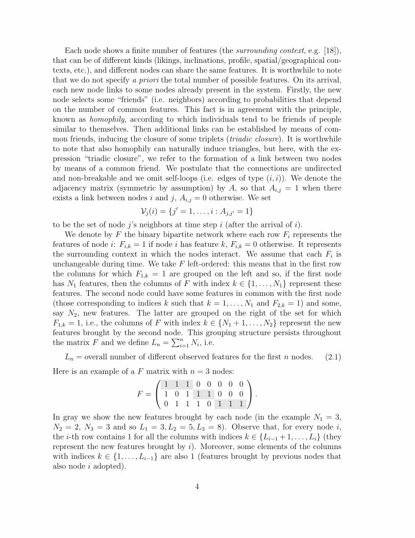
Here is an example of a F matrix with n = 3 nodes:

F =

1 1 1 0 0 0 0 01 0 1 1 1 0 0 00 1 1 1 0 1 1 1

.

In gray we show the new features brought by each node (in the example N1 = 3,N2 = 2, N3 = 3 and so L1 = 3, L2 = 5, L3 = 8). Observe that, for every node i,the i-th row contains 1 for all the columns with indices k ∈ {Li−1 +1, . . . , Li} (theyrepresent the new features brought by i). Moreover, some elements of the columnswith indices k ∈ {1, . . . , Li−1} are also 1 (features brought by previous nodes thatalso node i adopted).

4

3 The model

Fix α > 0, β ∈ [0, 1], δ ∈ [0, 1], and p ∈ [0, 1]. Moreover, let Φ : R → [0, 1] bean increasing function. The dynamics is the following. Node 1 arrives and showsN1 features, where N1 is Poi(α)-distributed (the symbol Poi(α) denotes the Poissondistribution with mean α). Then, for each i ≥ 2,

• Feature selection: Bipartite Network construction Node i arrives andshows a number of features as follows:

– Node i exhibits some of the “old” features brought by the previous nodes1, . . . , i − 1: more precisely, each feature k ∈ {1, . . . , Li−1} is, indepen-dently of the others, possessed by node i with probability (that we call“inclusion-probability”)

Pi(k) = δ1

2+ (1− δ)

∑i−1j=1 Fj,k

i, (3.1)

where Fj,k = 1 if node j shows feature k and Fj,k = 0 otherwise.

– Node i also shows Ni “new” features, where Ni is Poi(λi)-distributed with

λi =α

i1−β. (3.2)

(Ni is independent of N1, . . . , Ni−1 and of the exhibited “old” features.)The matrix element Fi,k is set equal to 1 if node i has feature k and equal tozero otherwise.

• (Unipartite) Network construction On its arrival, node i establishes aset Li of “friends” (i.e. neighbors) among the nodes already present in thenetwork (so that we set Ai,j = Aj,i = 1 for each j ∈ Li) as follows:

– (First phase) First, node i selects a set L∗i of friends on the basis of

the features shown. Each node j already present in the network (i.e.1 ≤ j ≤ i − 1) is included in L∗

i , independently of the others, withprobability

Φ(Si,j), (3.3)

where Si,j =∑Li

k=1 Fi,kFj,k is the number of features that i and j have incommon.

– (Second phase) Then some extra friends are added to Li on the basisof common friends. For every node j ∈ {1, . . . , i − 1} \ L∗

i , each nodej′ ∈ Vj(i − 1) ∩ L∗

i (i.e. each neighbor that i and j currently share)can induce, independently of the others, the additional link (i, j) withprobability p.

5

4 Meaning of the model parameters and some re-

sults

We now illustrate the meaning of the model parameters and some mathematicalresults regarding our model.

4.1 The parameters α and β

Let us start with α and β. The main effect of β is to regulate the asymptoticbehavior of the random variable Ln defined in (2.1). In particular, β > 0 is thepower-law exponent of Ln as a function of n. The main effect of α is the following:the larger α, the larger the total number of new features brought by a node. It isworth to note that β fits the asymptotic behavior of Ln (in particular, the power-lawexponent of Ln) and then, separately, α fits the number of new observed featuresper node. In Section 6.1 we will discuss more deeply this fact.

More precisely, we prove (see the Appendix) the following asymptotic behaviors:

a) for β = 0, we have a logarithmic behavior of Ln, that is Ln/ln(n)a.s.−→ α;

b) for β ∈ (0, 1], we obtain a power-law behavior, i.e. Ln/nβ a.s.−→ α/β.

4.2 The parameter δ

The parameter δ tunes the phenomenon of preferential attachment in the spreadingprocess of features among nodes. The value δ = 0 corresponds to the “pure prefer-ential attachment case”: the larger the weight of a feature k at time step i−1 (givenby the numerator of the second element in (3.1), i.e., the total number of nodes thatexhibit it until time step i − 1), the greater the probability that k will be shownby the future node i. The value δ = 1 corresponds to the “pure i.i.d. case” withinclusion probability equal to 1/2: a node includes each feature with probability 1/2independently of the other nodes and the other features. When δ ∈ (0, 1), we have amixture of the two cases above: the smaller δ, the more significant is the role playedby preferential attachment in the transmission of the features to new nodes.

4.3 The function Φ and the parameter p

According to our model, when a new node enters the system, it selects some (possiblyzero, one, or more) old nodes to whom link by means of the two phases networkconstruction described in Section 3.

In the first phase, a new node i connects itself to some old nodes according tothe probability function Φ, that depends on its own features and the ones of theothers. Indeed, the features provide the surrounding context in which the nodes

6

interact. The function Φ relates the “first-phase link-probability” of i to j (with1 ≤ j ≤ i− 1) to their “similarity” Si,j defined as

Si,j = number of features that i and j have in common =

Li∑

k=1

Fi,kFj,k. (4.1)

Since Φ is assumed to be an increasing function, a higher number of common featuresbetween nodes i and j induces a larger probability for them to connect (akin theprinciple of homophily).

In the second phase, node i can connect to some of the nodes discarded in the firstphase by means of common “friends” (i.e. neighbors). The parameter p regulatesthis phenomenon, known as triadic closure. Indeed, it represents the probability thata node j′ causes a link between two of its neighbors. Consequently, the “second-phase link-probability” between a pair of nodes increases with respect to p and thenumber of neighbors they share.

Combining together these two phases, we obtain that the probability that a newnode i links to a node j already present in the network is given by

πi,j = Φ(Si,j) + [1− Φ(Si,j)][1− (1− p)Ci,j

]

= 1− [1− Φ(Si,j)] (1− p)Ci,j ,(4.2)

where Ci,j = card(Vj(i − 1) ∩ L∗

i

)is the number of common neighbors of i and j

after the first phase. In particular, the second term of the above formula comes fromthe binomial distribution with parameters Ci,j and p. The case p = 0 correspondsto the case in which the connections only depend on the similarity among nodes.

Regarding the function Φ, we can take the generalization of the logistic function,i.e. the sigmoid function

Φ(s) =1

1 + eK(ϑ−s)with K > 0, ϑ ∈ R. (4.3)

The sigmoid function smoothly increases (from 0 to 1) around a threshold ϑ, whileK controls its smoothness: the bigger K, the steeper the sigmoid. In particular,K = 1 and ϑ = 0 give the logistic function and, for K → +∞, Φ approaches to astep function equal to 1 or 0, if the variable s is respectively greater or smaller thanϑ (in our model, ϑ ≥ 0 means that the links are established deterministically basedon whether the two involved nodes have, or not, a similarity bigger than ϑ).

We postpone the discussion about the estimation of the model parameters to thenext section.

5 Estimation of the model parameters

In this section we illustrate how to estimate the model parameters from the data.

7

Suppose we can observe the values of F1, . . . , Fn, i.e. n rows of the matrix F ,where n is the number of observed nodes. From the asymptotic behavior of Ln, weget that ln(Ln)/ ln(n) is a strongly consistent estimator for β, hence we can use the

slope β of the regression line in the log-log plot (of Ln as a function of n) as anestimate for β.

After computing β, we can estimate α as:

α = γ when β = 0

α = β γ when 0 < β ≤ 1,(5.1)

where γ is the slope of the regression line in the plot(ln(n), Ln

)or in the plot(

nβ, Ln

)according to whether β = 0 or β ∈ (0, 1].

We can estimate δ by means of a maximum likelihood procedure. For thispurpose, we now give a general expression of the probability of observing F1 =f1, . . . , Fn = fn given the parameters α, β, and δ.

The first row F1 is simply identified by L1 = N1 and so

P (F1 = f1) = P (N1 = n1 = card{k : f1,k = 1})

= Poi(α){n1} = e−ααn1

n1!.

Then the second row is identified by the values F2,k, with k = 1, . . . , L1 = N1, andby N2, so that

P (F2 = f2|F1) =

P (F2,k = f2,k for k = 1, . . . , L1, N2 = n2 = card{k > L1 : f2,k = 1}|F1) =

L1∏

k=1

P2(k)f2,k(1− P2(k))

1−f2,k × Poi(λ2){n2},

where P2(k) is defined in (3.1) and λ2 is defined in (3.2). The general formula is

P (Fi = fi|F1, . . . , Fi−1) =

P (Fi,k = fi,k for k = 1, . . . , Li−1,

Ni = ni = card{k > Li−1 : fi,k = 1}|F1, . . . , Fi−1) =

Li−1∏

k=1

Pi(k)fi,k(1− Pi(k))

1−fi,k × Poi(λi){ni},

where Pi(k) is defined in (3.1) and λi is defined in (3.2). Thus, for n nodes, we canwrite a formula for the probability of observing F1 = f1, . . . , Fn = fn:

P (F1 = f1, . . . , Fn = fn) =

P (F1 = f1)n∏

i=2

P (Fi = fi|F1, . . . , Fi−1).(5.2)

8

Therefore, we look for δ that maximizes the likelihood function, i.e. the quantityP (F1 = f1, . . . , Fn = fn) as a function of δ (given the observed vectors fi). Sincesome factors do not depend on δ, we can simplify the function to be maximized as

n∏

i=2

Li−1∏

k=1

Pi(k)fi,k(1− Pi(k))

1−fi,k , (5.3)

or, equivalently, passing to the logarithm, as

n∑

i=2

Li−1∑

k=1

fi,k ln(Pi(k)

)+ (1− fi,k) ln

(1− Pi(k)

). (5.4)

Now, suppose that we are also allowed to observe the adjacency matrix A =(Ai,j)1≤i,j≤n (meaning the final adjacency matrix after the arrival of all the n ob-served nodes and the formation of all their links) and to know which are the linksthat each of the n observed nodes formed only by means of the previously describedfirst phase (i.e. only due to homophily). Denote by A′ = (A′

i,j)1≤i,j≤n the adjacencymatrix collecting them. Then, if we decide to model the function Φ as in (4.3), wecan choose K, ϑ, and p, in order to fit some properties of the observed matrices A′

and A.

For instance, if ℓ is the number of observed (undirected) links in matrix A′ (i.e.only due to the first phase of network construction) and

f ∗ =observed number of linked (in A′) pairs of nodes with s∗ features in common

observed number of pairs of nodes with s∗ features in common,

where s∗ is a fixed value that we choose, then we can determine K > 0 and ϑ ∈ R

by solving (numerically) the following system of two equations:

Φ(s∗) =(1 + eK(ϑ−s∗)

)−1= f ∗

E

[∑

i,j:2≤i≤n,1≤j≤i−1

A′i,j

]=

n∑

i=2

i−1∑

j=1

Φ (Si,j) =

n∑

i=2

i−1∑

j=1

(1 + eK(ϑ−s∗)+K(s∗−

∑Lik=1

Fi,kFj,k))−1

= ℓ.

(5.5)

By means of the the first equation, we fit the probability that a pair of nodes withs∗ features in common establishes a link (during the first phase of network construc-tion); while, by the second equation, we set the expected number of links in A′ equalto the observed ℓ. From the first equation, we get the quantity K(ϑ− s∗), we thenreplace it in the second one in order to obtain K and from this we get ϑ. Note that

9

this is not a proper estimation procedure, but rather a selection mechanism for Kand ϑ in order to fit some observed properties of the network.

After that, we can estimate p by means of a maximum likelihood procedure.Specifically, we can find p that maximizes the following probability as a function ofp (given the observed matrices F,A′, A):

P (Ai,j = ai,j, ∀1 ≤ i ≤ n, 1 ≤ j ≤ i− 1) =n∏

i=1

i−1∏

j=1

πai,ji,j (1− πi,j)

1−ai,j ,

where πi,j is given by (4.2) with Ci,j = card(Vj(i−1)∩L∗

i

)= card

({j′ = 1, . . . , i−1 :

Aj,j′ = 1, A′i,j′ = 1}

).

Some important remarks follow.

• If in the considered situation the formation of links only occurs according tothe first phase (i.e. according to homophily), then we can set p = 0 as inthis case the presence of triangles is only caused by common features andthe matrix A coincides with A′. Then we have no problem to implement theprevious procedures for detecting all the model parameters.

• When we have both phases of network construction (i.e. p > 0), the detectionof K,ϑ, and p may generate some problems since the available data are typi-cally F and A, while, in order to implement the above procedure, we also needto observe A′. Hence, when we cannot observe A′, we may try to reconstructit from A in some consistent way, if it is possible for the considered application[36]. However, every empirical criterion used to distinguish between the twodifferent types of links (the ones due to the first phase and the ones inducedby the second phase), obviously has some degree of arbitrariness and it can behard to understand the bias implied by it. An example of this problem can befound in [13] regarding a citation network. In the case no suitable criterion isfound, we may try to select K,ϑ, and p in such a way that some properties ofthe adjacency matrix generated by the model are close to the observed one.The simulation of the model with the observed matrix F and p = 0 is stilluseful as a benchmark.

6 Simulations

In this section, we present a number of simulations performed following the dynamicsfor the features’ selection and links’ creation described in Section 3. We simulatedthe outcome for feature matrices and for unipartite networks of 1000 nodes, on asample of 100 repetition steps (realizations).

10

Regarding the feature-selection dynamics, we analyzed the resulting feature ma-trices (constructed as explained in Section 2) for different values of the model para-meters α, β, and δ, responsible respectively of the number of new features per node,the asymptotic behavior of Ln, and the phenomenon of preferential attachment inthe transmission of the features to new nodes. After that, we simulated the networkconstruction taking Φ as in (4.3) and analyzed its properties for different values ofδ, K, and p, while ϑ is determined according to a certain number ℓ of (undirected)links due to the first phase of the unipartite network construction.

6.1 Simulations of the feature matrix and estimation of α, β,and δ

As said before, parameter α is responsible for the number of new features per node:the larger α, the higher the number of new features per node. Concerning this, it isvery important to stress that also the parameter β affects the number of features pernode, but the idea is that we select first β, in order to fit the asymptotic power-lawbehavior of Ln defined in (2.1), and then α in order to fit the number of new featuresper node.

In the first set of simulations we kept β = 0.5 and δ = 0.1 fixed and we built thefeature matrix for different values of α = 3, 8, 13. In Figure 1 we can see the shapesof the feature matrices (where colored points denote non-zero values, i.e. 1) for thethree different values of α. It is immediate to see that the main difference amongthese matrices concerns the number of features: the total number of features is 185for α = 3, 533 for α = 8, and 819 for α = 13. Correspondingly, the mean numberof new features per node (averaged over 100 realizations) is about 0.19 for α = 3,0.49 for α = 8, and 0.8 for α = 13. The mean number of (total) adopted featuresper node (averaged over 100 realizations) is about 19.99 for α = 3, 52.66 for α = 8,and 79.65 for α = 13.

In Figure 2 we show the estimates for the different values of α (with β = 0.5 andδ = 0.1 kept fixed).

Parameter β controls the asymptotic behavior of Ln defined by (2.1). For thisreason we plotted Ln as a function of n in a log-log scale, results are reported inFigure 3. In Figure 3 (a)-(b), we show the estimates for two different values of β(β = 0.75 and β = 1), with α = 3 and δ = 0.1. In Figure 3 (c)-(d), we show theestimate of β, for β = 0.5 and β = 0.75, but for a different value of α (α = 10) inorder to underline that α does not affect the power-law behavior of Ln (obviously,the value of the estimate can be more or less accurate for different values of α).

Finally, parameter δ regulates the phenomenon of preferential attachment: δ = 0corresponds to the pure preferential attachment case; while δ = 1 to the pure i.i.d

11

Figure 1: An example of features matrices for n = 1000, β = 0.5, δ = 0.1, anddifferent values of α : 3 (left), 8 (middle), 13 (right). Colored points denote 1 andwhite points denote 0.

Figure 2: Estimates of α (when β = 0.5 and δ = 0.1) obtained as the slope of theregression line in the plot of Ln as a function of nβ. Different values of α : 3 (left),8 (middle), 13 (right) are reported.

12

(a) (b)

(c) (d)

Figure 3: Estimates of β obtained as the slope of the regression line in the log-logplot of Ln as a function of n. Different values of α and β are reported: α = 3, β =0.75 (a), α = 3, β = 1 (b), α = 10, β = 0.75 (c), and α = 10, β = 0.5 (d).

13

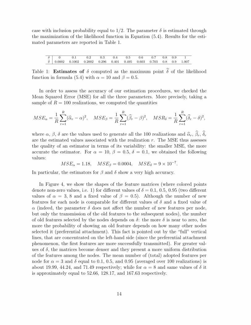
case with inclusion probability equal to 1/2. The parameter δ is estimated throughthe maximization of the likelihood function in Equation (5.4). Results for the esti-mated parameters are reported in Table 1.

δ 0 0.1 0.2 0.3 0.4 0.5 0.6 0.7 0.8 0.9 1

δ 0.0002 0.1002 0.2002 0.296 0.401 0.495 0.603 0.703 0.8 0.9 1.007

Table 1: Estimates of δ computed as the maximum point δ of the likelihoodfunction in formula (5.4) with α = 10 and β = 0.5.

In order to assess the accuracy of our estimation procedures, we checked theMean Squared Error (MSE) for all the three parameters. More precisely, taking asample of R = 100 realizations, we computed the quantities

MSEα =1

R

R∑

r=1

(αr − α)2, MSEβ =1

R

R∑

r=1

(βr − β)2, MSRδ =1

R

R∑

r=1

(δr − δ)2,

where α, β, δ are the values used to generate all the 100 realizations and αr, βr, δrare the estimated values associated with the realization r. The MSE thus assessesthe quality of an estimator in terms of its variability: the smaller MSE, the moreaccurate the estimator. For α = 10, β = 0.5, δ = 0.1, we obtained the followingvalues:

MSEα = 1.18, MSEβ = 0.0004, MSEδ = 9× 10−7.

In particular, the estimators for β and δ show a very high accuracy.

In Figure 4, we show the shapes of the feature matrices (where colored pointsdenote non-zero values, i.e. 1) for different values of δ = 0.1, 0.5, 0.95 (two differentvalues of α = 3, 8 and a fixed value of β = 0.5). Although the number of newfeatures for each node is comparable for different values of δ and a fixed value ofα (indeed, the parameter δ does not affect the number of new features per node,but only the transmission of the old features to the subsequent nodes), the numberof old features selected by the nodes depends on δ: the more δ is near to zero, themore the probability of showing an old feature depends on how many other nodesselected it (preferential attachment). This fact is pointed out by the “full” verticallines, that are concentrated on the left-hand side (since the preferential attachmentphenomenon, the first features are more successfully transmitted). For greater val-ues of δ, the matrices become denser and they present a more uniform distributionof the features among the nodes. The mean number of (total) adopted features pernode for α = 3 and δ equal to 0.1, 0.5, and 0.95 (averaged over 100 realizations) isabout 19.99, 44.24, and 71.49 respectively; while for α = 8 and same values of δ itis approximately equal to 52.66, 128.17, and 167.63 respectively.

14

Figure 4: Examples of features matrices for n = 1000, β = 0.5, different valuesof α : 3 (up), 8 (below) and different values of δ : 0.1 (left), 0.5 (middle), 0.95 (right).Colored points denote 1 and white points denote 0.

In order to “measure” the “uniformity” of the distribution of the features amongnodes, we simply divided the total set of the features into two subsets: {1, . . . , ⌊Ln/2⌋}and {⌊Ln/2⌋+1, . . . , Ln}. For each feature, we computed the mean number of nodesthat adopted it (i.e. the total number of nodes that adopted the considered featuredivided by the total number of nodes that could have adopted it). Then we com-puted the mean value of these numbers over the two subsets and took the differencebetween these two values. For different values of α and δ, Table 2 contains the corre-sponding values (averaged over 100 realizations) of these differences. It is clear thatthe smaller the reported value, the more uniform is the distribution of the featuresin the matrix. We can notice that for δ = 0.1 and δ = 0.5 the obtained values arecomparable (about 0.10 and 0.11); while for δ = 0.95 we got a very small value.

δ = 0.1 δ = 0.5 δ = 0.95α = 3 0.1005 0.1119 0.0099α = 8 0.1010 0.1129 0.0097

Table 2: Measure of the “uniformity” of the feature matrix defined as thedifference (averaged over 100 realizations) between the mean number of nodes perfeature for the first and the second half of the features’ set. Considered parameters:α = 3, 8, β = 0.5 and δ = 0.1, 0.5, 0.95.

15

6.2 Simulations of the unipartite network and procedure in

order to recover K and ϑ

We performed the simulations of the unipartite network as follows. Once a featurematrix F is generated, links are created according to the two phases of the linkconstruction described in Section 3, taking Φ as in (4.3). We simulated the networkfor n = 1000 nodes on a sample of 100 repetition steps (realizations).

In the first set of experiments, we fixed a number ℓ and, for different values ofK > 0 (one of the parameters of the function Φ), we determined the value of ϑsolving (numerically) the equation

n∑

i=2

i−1∑

j=1

(1 + eK(ϑ−

∑Lik=1

Fi,kFj,k))−1

= ℓ , (6.1)

in order to have the expected number of (undirected) links due to the first phase ofthe unipartite network construction equal to the given number ℓ. Hence, we studiedthe network structure as a function of the parameters K and p (related to the linkformation). In particular, we recall that p increases the triadic closure phenomenon.We also considered different values of δ, that regulates the preferential attachmentin the transmission of the features and so influences the shape of the feature matrixF . In the Appendix we report the results.

With the second set of experiments, we studied the accuracy of procedure (5.5) inorder to recover K and ϑ. Hence, we fixed α = 10, β = 0.5, δ = 0.1, K = 1, ϑ = 10,and p = 0 (so that A′ = A) and we generated a sample of R = 100 realizations of thenetwork. We then applied the procedure (5.5) to each realization r (with s∗ = 10)

in order to get the corresponding values Kr and ϑr. The procedure results accurate.Indeed, we found:

1

R

R∑

r=1

Kr = 1.000462, MSEK =1

R

R∑

r=1

(Kr −K)2 = 0.00415,

1

R

R∑

r=1

ϑr = 9.998843, MSEϑ =1

R

R∑

r=1

(ϑr − ϑ)2 = 0.00010.

7 Application to a co-authorship network

In order to analyze (by means of our model and related statistical tools) the inter-action between features and social relations in a real world dataset, we downloadedbibliographic information of papers and preprints found in the IEEE Xplore database[59]. In this dataset a social relation is taken as the co-authorship of a paper betweentwo or more authors and the contexts of the papers are given by 2-grams (pairs of

16

sequential words in the title or abstract). We selected the papers using search termsrelated to the specific research area of autonomous cars (also called connected cars).The understanding of homophily and triadic closure in co-authorship networks isvery important since these two phenomena can affect the diffusion process of ideasand discoveries inside a certain research field and among different research fields[4, 21, 46].

7.1 Description of the dataset

We downloaded (on Aug. 7, 2014) all papers in the IEEE preprint and paper archiveusing 17 specific search terms: ‘Lane Departure Warning’, ‘Lane Keeping Assist’,‘Blindspot Detection’, ‘Rear Collision Warning’, ‘Front Distance Warning’, ‘Au-tonomous Emergency Braking’, ‘Pedestrian Detection’, ‘Traffic Jam Assist’, ‘Adap-tive Cruise Control’, ‘Automatic Lane Change’, ‘Traffic Sign Recognition’, ‘Semi-Autonomous Parking’, ‘Remote Parking’, ‘Driver Distraction Monitor’, ‘V2V or V2Ior V2X’, ‘Co-Operative Driving’, ‘Telematics & Vehicles’, and ‘Night vision’. TheIEEE archive returned all the papers in their database that contain these terms inthe title or abstract, and we downloaded the bibliographic records for all returnedpapers including the authors, title, abstract, and the date on which the paper wasadded to the database. This download yielded 6 129 distinct papers with a completebibliographic record and at least two authors. While these search terms can not beexpected to yield all papers related to automated car research, we expect to havefound a relatively broad panel of related papers.

7.2 Analysis of the feature matrix

The feature matrix was built by extracting all 2-grams (pairs of words) appearing ineither the title or abstract of a paper. The text was converted to lowercase, removingall punctuation (with the exception of the ‘/’ and ‘.’ characters) and multi-spaces,and split into individual sentences. The 2-grams occurring in any sentence in thetitle or abstract were labeled as features of the paper. In order to remove spurious2-grams (e.g. ‘this paper’ often occurs in the abstract, but it is not relevant toconnected cars), we exclude any 2-grams containing any of the words: ‘the’, ‘a’,‘of’, ‘and’, ‘to’, ‘is’, ‘for’, ‘in’, ‘an’, ‘with’, ‘by’, ‘from’, ‘on’, ‘or’, ‘that’, ‘at’, ‘be’,‘which’, ‘are’, ‘as’, ‘one’, ‘may’, ‘it’, ‘and/or’, ‘if’, ‘via’, ‘can’, ‘when’, ‘we’, ‘his’,‘her’, ‘their’, ‘this’, ‘our’, ‘into’, ‘has’, ‘have’, ‘only’, ‘also’, ‘do’, ‘does’, ‘presents’,‘paper’, ‘doesn’t’, and ‘not’. This approach gave 155 897 distinct 2-grams (features)for a total of 6 129 papers (nodes). We ordered the papers chronologically based ontheir entry date into the IEEE database (which we expect to be a good proxy fortheir publication date). The 2-grams were ordered in terms of their first appearancein a paper (as described in Sec. 2). For the 2-grams that appear for the first timein the same paper, we chose to order them in terms of how commonly they occur: amore common 2-gram precedes a less common 2-gram. However this last ordering

17

(a)

Features

Art

icle

s

1 5000 10000 15000 20000 250001000

700

350

1

(b)

Figure 5: (a) Feature-matrix associated to the dataset. Dimensions: 6 129 nodes(papers) × 155 897 features (2-grams). Colored points denote 1 and white pointsdenote 0. (b) Feature matrix for 1000 nodes, obtained by simulation of the model

with α = α = 32.28, β = β = 0.98, and δ = δ = 0.0057. Colored points denote 1 andwhite points denote 0. The total number of features is 28 664, which is consistentwith the observed matrix.

is irrelevant for our analysis.

Having extracted the set of the 2-grams contained in each paper, we constructedthe feature-matrix F , with Fik = 1 if paper i contains the 2-gram k and Fik = 0otherwise. The resulting matrix F is shown in Fig. 5(a), with non-zero values ofF indicated by colored points. We also simulated the feature-matrix for a smallernetwork of 1000 nodes taking the parameters equal to the corresponding estimatedvalues (see Fig. 5(b)). The number of features obtained in the simulation is 28 664,which is consistent with the observed matrix.

The growth of the cumulative count Ln of the distinct 2-grams (the numberof distinct 2-grams seen until the nth paper included, as described in Section 2)is shown in Fig. 6(b) in a log-log scale and it shows a clear power-law behavior,

with estimated parameter β = 0.98 (that corresponds to the estimated value of themodel parameter β). Regarding the model parameter α, we get the estimated valueα = 32.28 and in Fig. 6(a) we show the corresponding fit plotting the cumulative

count Ln of the 2-grams as a function of nβ. Finally, the estimated value for the

18

Figure 6: Estimated values of the model parameters α and β.

parameter δ is δ = 0.0057. As we can see, this last value is very small and so we canconclude that the preferential attachment rule in the transmission of the featuresplays an important role.

7.3 Analysis of the unipartite network

Our dataset includes 6 129 papers for a total of 13 581 distinct author names. Theconsidered unipartite network is constructed taking the papers as nodes and draw-ing a link between two nodes if they share at least one author. We harmonized theauthor names across different papers by ensuring that the authors’ last names arealways found in the same position and removed any stray punctuation in the names.No further disambiguation was performed, meaning that authors who may use theirfull names in some papers but only their initials in other papers will be treated asdistinct. For example, the names “J. J. Anaya” and “Jose Javier Anaya” are treatedas distinct authors in our dataset, while it is possible that these distinct names re-fer to the same person. A full disambiguation of author names is computationallydifficult [37], and beyond the scope of this paper. This approach gave a unipartitenetwork with 19 065 links that involve 4 712 nodes in the network. This means thatthere are 1 417 isolated nodes, where the paper has two or more authors that arenot listed on any other paper in the dataset. However, we decided to consider alsothese nodes in our analysis since we included them in the features matrix as nodesthat can potentially link to other nodes.

The distribution of the 2-grams (the features) in common between two papers(the nodes) given the presence or the absence of at least one shared author (i.e.given the presence or the absence of a link between them) is plotted in Figure 7(a).The (blue) circles-curve is the distribution of the number of 2-grams shared by twopapers given they have at least one co-author. More precisely, for each value on the

19

x-axis, we have on the y-axis the fraction

num. of pairs of papers with x 2-grams in common and at least 1 shared author

num. of pairs of papers with at least 1 shared author.

(7.1)The (black) squares-curve is the distribution of the number of 2-grams shared bytwo papers given they have no authors in common, i.e. we have the same formulaas (7.1) but with pairs of papers without shared authors. As we can see, there is amuch higher probability of common 2-grams if there are shared authors. This factsuggests the presence of homophily.

The fraction of pairs of papers with x 2-grams (the features) in common thathave at least one shared author (the linked pairs of nodes) is plotted in Figure 7(b).More precisely, for each value on the x-axis, we have on the y-axis the fraction

num. of pairs of papers with x 2-grams in common and at least 1 shared author

num. of pairs of papers with x 2-grams in common.

(7.2)As we can see, the plotted fraction increases with the number of features in common.This fact again suggests the presence of homophily.

The clustering coefficient (see formula (A.1)) is also fairly high, C = 78%, indi-cating the presence of a significant triadic closure phenomenon.

The network is composed of 586 connected components with at least one edgeand 1 417 isolated nodes (a total of 2 003 components). The largest connected com-ponent has 2 776 nodes and 16 108 links, so about the 45% of the nodes can reacheach other in the largest connected component and it includes about the 84% ofthe links. The diameter (i.e. the maximum distance between nodes) of the largestconnected component is 23. The other 585 connected components (disconnectedfrom the largest component but still having at least one edge) globally contain 1 936nodes, and over 90% of the components (containing over 75% of the nodes outsideof the largest connected component) contain 7 or fewer nodes. Hence the percentageof reachable pairs (denoted by RP in the remainder of the paper) of nodes in thenetwork is about 20.51%.

As discussed in Section 5, since we have only the final adjacency matrix, we cannot estimate the parameter p, i.e. the parameter governing triadic closure. Hence,we decided to first use the model with p = 0 in order to have a benchmark and thentry to guess a good value for p.

Taking p = 0, we set A′ = A (i.e. links are only formed by means of the firstphase) and we applied the procedure (5.5) to the observed feature-matrix F withs∗ = 10 (the corresponding value for f ∗ is 0.725) and ℓ = 19 065 in order to detect

K and ϑ: we found K = 0.8228 and ϑ = 8.8201. We then generate a sample of100 realizations of the network by simulating the model starting from the observed

20

matrix F and with p = 0, K = K = 0.8228, and ϑ = ϑ = 8.8201. We also com-puted the percentage of reachable pairs (RP = 99%) and the clustering coefficient(C = 0.69%), but we found values that are very different from the observed ones.This can be obviously explained by the fact that we set p = 0 (benchmark case),while a value of p strictly greater than 0 is guessable.

Setting p = 0.7 and generating a sample of 100 realizations of the network bysimulating the model starting from the observed matrix F 1, we succeeded to cap-ture a value for RP very near to the observed one, i.e. RP = 19.61% (this valueis an average over the 100 realizations). Moreover, we obtained that the biggestconnected component contains on average 2 689.16 nodes. Finally, Figure 7(c) and(d) contain, respectively, the distribution of the features in common between twonodes given the presence (blue circles) or the absence (black triangles) of a linkbetween them and the fraction of pairs of nodes with x features in common that arelinked. These distributions properly fit the observed ones. However, as concerns theclustering coefficients, we found C = 39%, which is smaller than the observed one.We then simulated the model with p = 0.8 2 and so we obtained a bigger value forthe clustering coefficient (C = 46%), but RP = 11%.

We thus guess that the best choice for the model parameter p is a value around0.7. However, this empirical analysis shows that, although our model is perfectlyable to reproduce the evolution of the feature-matrix, to explain homophily and tocapture the value of some network indicators, we need to take into account possiblevariants of the model in order to explain very high values of clustering coefficient.We postpone to Section 8 the discussion on possible improvements of our model.

8 Conclusions and discussion on some variants of

the model

In this paper, we presented a new network model, especially suitable to describesocial interactions. In our model, each node is characterized by a number of fea-tures (i.e. the surrounding context) and the probability of a link between two nodesdepends on the number of features and friends (i.e. neighbors) they share, so that itincludes two of the most observed phenomena in social systems: homophily (meantas the tendency of individuals to be friends of people similar to themselves) andtriadic closure (meant as the formation of a link between a pair of nodes by means

1In this case we took into account that A′ is different from A, and so the parameters K and ϑ

used for the simulations were recovered by applying the procedure (5.5) to the observed feature-matrix F with a smaller ℓ (that corresponds to the expected number of links formed during the firstphase). We set ℓ = 4000 in order to have an averaged total number of links around the observed

one. We did not change the values for s∗ and f∗. We found K = 1.019574 and ϑ = 9.047858.2In this case, we used ℓ = 3500 in order to have an averaged total number of links around the

observed one (and the same values for s∗ and f∗) and we recovered K = 1.039748 and ϑ = 9.066332.

21

æ

æ

æ

æ

ææ

æææææææææææææææææææ

æ

ææ

æææ

æ

ææææ

ææææ

æææææææ

ææ

æ

æ

ææææ

æ

ææ

ææ

æ

æææææ

à

à

à

à

à

à

à

à

à

à

àà

à

à

àààààààà

ààà

à

à

à

àààààààà

1 2 5 10 20 50

10-7

10-5

0.001

0.1

features in common

fracti

on

(a) (b)

à

à

à

à

à

à

à

à

à

à

à

à

à

àà

æ

æ

ææ

æææææ æ

ææææææææææ

æææææ

æ

ææ

ææææææææ

ææ

ææ

æ

æææ

æææ

æ

æ

æ

æ

1 2 5 10 20 50

10-7

10-5

0.001

0.1

features in common

fracti

on

(c)

ììììììì

ì

ì

ì

ì

ìììììììììììììììììììììììì

0 5 10 15 20 25 30 35

0.0

0.2

0.4

0.6

0.8

1.0

features in common

fracti

on

wit

hcoauth

or

(d)

Figure 7: (a) The distribution of the 2-grams (features) in common between twopapers (nodes) given the presence (blue circles) or the absence (black squares) of atleast one co-author. (b) The fraction of pairs of papers with x 2-grams in commonthat have at least one co-author. (c) The same distribution in (a) but obtained bysimulation starting from the observed matrix F and setting p = 0.7 and ℓ = 4000(and averaged on 100 realizations). (d) The same fraction in (b) but obtained bysimulation starting from the observed matrix F and setting p = 0.7 and ℓ = 4000(and averaged on 100 realizations).

22

of common friends). The bipartite network of the features evolves according to adynamics that depends on three parameters respectively regulating the preferentialattachment in the transmission of the features to the nodes, the number of new fea-tures per node, and the power-law behavior of the total number of observed features.We provide theoretical results and statistical tools for the estimation of the modelparameters involved in the feature-selection dynamics. From the observation of thefeature-matrix, we completely determine the parameters that regulate its evolution.For the case in which the function Φ, which relates the link probability betweentwo nodes to their similarity in terms of common features, is modeled by a sigmoidfunction, we provide a procedure for recovering the related parameters. Moreover,we describe a way to estimate the parameter p that rules triadic closure. However,for the last point, we need to observe which are the links formed by homophily (firstphase) and those formed by triadic closure (second phase). Nevertheless, as shownin Section 7, when this information is not available, we can still exploit the proposedprocedure by varying p and the expected number ℓ of links due to homophily, andtry to guess a good combination of the parameters.

The originality and the merit of our model lie in the double temporal dynamics(one for the bipartite network of features and one for the unipartite network ofnodes), in the attention given to both homophily and triadic closure mechanisms,and in the related statistical estimators. However, our model could result inadequateto explain the whole clustering value in the case of some real networks with a veryhigh clustering coefficient. In the future, we aim at improving it by considering thefollowing variations:

• Normalizing the number of common features: A possible variation can be ob-tained by replacing the factor Fi,kFj,k in formula (4.1) with

Fi,kFj,k∑i−1j′=1 Fj′,k

, ∀(i, j) s.t. 1 ≤ j ≤ i− 1,

so that the contribution of a common feature k is smaller when the number ofnodes with k as a feature is larger.

• Weighted bipartite matrices: We can modify the model by replacing in theinclusion-probability and in the link-probability the binary random numberFi,k by a random weight Wi,k of the form Wi,k = Fi,kYi,k/(

∑Li

k=1 Fi,kYi,k), whereYi,k are i.i.d. strictly positive random variables. (By convention, we set 0/0 =0.) Hence, we have

Wi,k ∈ [0, 1] and

Li∑

k=1

Wi,k = 1

so that Wi,k represents the weight percentage given to feature k by node i.Therefore, the preferential attachment in the inclusion-probability becomes

23

a “weighted preferential attachment”, in the sense that it depends on thetotal weight given to feature k by the previous nodes, and the link-probabilitydepends on the weights associated to the common features.

• Social influence of links on features: In some real cases, a node could changesome features under the influence of its “friends/neighbors”. Hence, we canintroduce a sequence (F (i))i of bipartite matrices such that each F (i) providesthe features before the arrival of node i+1, so that in the inclusion-probabilitiesand in the link-probabilities for node i+ 1, the matrix F is replaced by F (i).

• Different dynamics for triadic closure: We can modify the second phase of ourmodel by means of different policies for the selection of additional “friends”of a node i among the friends of i’s friends. Indeed, in this paper we considera binomial model according to which each common friend of a pair (i, j) ofnot-linked nodes gives, independently of the others, a probability p of inducinga link between i and j. A possible alternative is that, with probability p, anadditional link for a certain node is formed by the selection (uniformly atrandom) of a node among the friends of its friends.

• Exit of some features and breakable links: We can modify the evolution of thefeatures matrix by accounting for the fact that at each time step j (after thearrival of the node j) some features can become “obsolete” and so for such afeature k we will have Fi,k = 0 for all i ≥ j + 1. For some real situations, weneed to consider also the case in which the links among nodes can break.

Acknowledgments and Financial Support

Authors acknowledge support from CNR PNR Project “CRISIS Lab”.

References

[1] Airoldi E., Blei D., Fienberg S. and Xing E. (2008) Mixed membership stochas-tic block-models. Journal of Machine Learning Research, 9, 1981-2014.

[2] Barabasi A. L. and Albert R. (2002) Statistical mechanics of complex net-works. Reviews of modern physics 74, 47-97.

[3] Barabasi A. L. and Albert R. (1999) Emergence of scaling in random networks.Science 286, 509-512.

[4] Barabasi A. L., Jeong H., Neda Z., Ravasz E., Schubert A. and Vicsek T.(2002) Evolution of the social network of scientific collaborations. Physica A,311, 590-614.

24

[5] Barrat A., Barthlemy M. and Vespignani A. (2008) Dynamical processes oncomplex networks. Cambridge University Press.

[6] Berti P., Crimaldi I., Pratelli L. and Rigo P. (2015) Central Limit Theoremsfor an Indian Buffet Model with Random Weights. The Annals of AppliedProbability 25(2), 523-547.

[7] Bessi A., Caldarelli G., Del Vicario M., Scala A. and Quattrociocchi W. (2014)Social determinants of content selection in the age of (mis)information. Pro-ceedings of SOCINFO 2014; abs/1409.2651.

[8] Bessi A., Coletto M., Davidescu G. A., Scala A., Caldarelli G. and Quattro-ciocchi W. (2015) Science vs Conspiracy: collective narratives in the age of(mis)information. Plos One 10, e0118093.

[9] Blau P.M. and Schwartz J.E. (1984) Crosscutting social circles: testing amacrostructural theory of intergroup relations, Academic Press, Orlando (FL).

[10] Bianconi G., Darst R. K., Iacovacci J. and Fortunato S. (2014) Triadic closureas a basic generating mechanism of communities in complex networks. PhysicalReview E, 90(4), 042806.

[11] Block P. and Grund T. (2014) Multidimensional homophily in friendship net-works. Network Science, 2(02), 189-212.

[12] Boldi P., Crimaldi I. and Monti C. (2014) A Network Model Characterized by aLatent Attribute Structure with Competition. Submitted. Currently availableon arXiv (1407.7729, 2014).

[13] Bramoulle Y., Currarini S., Jackson M. O., Pin P. and Rogers B. W. (2012)Homophily and long-run integration in social networks. Journal of EconomicTheory, 147(5), 1754-1786.

[14] Brown J., Broderick A. J. and Lee N. (2007) Word of mouth communicationwithin online communities: Conceptualizing the online social network. Journalof interactive marketing, 21(3), 2-20.

[15] Caldarelli G. (2007) Scale-Free Networks: complex webs in nature and tech-nology. OUP Catalogue.

[16] Currarini S., Jackson M. O. and Pin P. (2009) An economic model of friend-ship: Homophily, minorities, and segregation. Econometrica, 77(4), 1003-1045.

[17] Currarini S. and Vega-Redondo F. (2013) A simple model of homophily insocial networks. University Ca’Foscari of Venice, Dept. of Economics ResearchPaper Series, (24).

25

[18] Easly D. and Kleinberg J. (2010) Networks, Crowds and Markets: Reasoningabout a Highly Connected World. Cambridge Univ. Press.

[19] Feld S.L. (1982) Social structural determinants of similarity among associates.American Sociological Review, 47(6), 797-801.

[20] Goldenberg A. and Zhen E. (2009) A survey of statistical network models.Foundations and trends in Machine Learning, 2, 129-233.

[21] Golub B. and Jackson M. O. (2009) How homophily affects the speed of learn-ing and best response dynamics. Quart. J. Econ., forthcoming.

[22] Handcock M. S., Raftery A. E. and Tantrum J. M. (2007) Model-based clus-tering for social networks. Journal of the Royal Statistical Society, series A,170, 301-354.

[23] Hoff P. D., Raftery A. E. and Handcock M. S. (2002) Latent space approachesto social network analysis. J. American Statistical Ass., 97, 1090-1098.

[24] Holme P. and Kim B. J. (2002) Growing scale-free networks with tunableclustering. Phys. Rev. E, 65(2).

[25] Hunter D. R., Krivitsky P. N. and Schweinberger M. (2012) Computationalstatistical Methods for Social Network Models. J. comput. Graph Stat., 21(4),856-882.

[26] Ispolatov I., Krapivsky P. L. and Yuryev A. (2005). Duplication-divergencemodel of protein interaction network. Phys. Rev. E., 71(6).

[27] Jackson M.O. (2014) Networks in the understanding of economic behaviors,The Journal of Economic Perspectives (2014), 3-22.

[28] Jackson M. O. (2008). Social and Economic Networks. Princeton UniversityPress.

[29] Jackson M.O. and Rogers B.W. (2007) Meeting strangers and friends offriends: How random are social networks? The American economic review,97(3), 890-915.

[30] Jackson M. O., Rogers B. W. and Zenou Y. (2015) The Economic Conse-quences of Social Network Structure. Available at SSRN.

[31] Kandel D.A. (1978) Homophily, selection, and socialization in adolescentfriendships, American Journal of Sociology, 84(2), 427-436.

[32] Kolaczyk E. D. (2009) Statistical analysis of network data: methods and mod-els. Springer.

26

[33] Kossinets G. and Watts, D. J. (2009) Origins of homophily in an evolvingsocial network. American Journal of Sociology, 115(2), 405-450.

[34] Kossinets G. and Watts D. J. (2006) Empirical Analysis of an Evolving SocialNetwork. Science 311.

[35] Krivitsky P. N., Handcock M. S., Raftery A. E. and Hoff P. (2009) Repre-senting degree distributions, clustering and homophily in social networks withlatent cluster random effects models. Social Networks, 31, 204-213.

[36] La Fond T. and Neville J. (2010) Randomization Tests for distinguishing SocialInfluence and Homophily Effects. International World Wide Web Conference.

[37] Lai R., Doolin D. M., Li G. C, Sun Y., Torvik V. and Yu A. (2014) Disam-biguation and Co-authorship Networks of the U.S. Patent Inventor Database.Research Policy 43, 941-955.

[38] Lazarsfeld P.F. and Merton R.K. (1954) Friendship as a social process: A sub-stantive and methodological analysis. Freedom and control in modern society,18(1), 18-66.

[39] Louch H. (2000) Personal network integration: transitivity and homophily instrong-tie relations. Social networks, 22(1), 45-64.

[40] Marsden P.V. (1987) Core discussion networks of Americans, American Soci-ological Review, 52(1), 122-131.

[41] Marsili M., Vega-Redondo F. and Slanina F. (2004) The rise and fall of anetworked society: A formal model. Proceedings of the National Academy ofSciences of the United States of America, 101(6), 1439-1442.

[42] McPherson M., Smith-Lovin L. and Cook, J. M. (2001) Birds of a feather:Homophily in social networks. Annual review of sociology, 27, 415-444.

[43] Miller K. T., Griffiths, T. L. and Jordan, M. I. (2009) Nonparametric LatentFeature Models for Link Prediction. In NIPS, Curran Associates, Inc., 1276-1284.

[44] Mocanu D., Rossi L., Zhang Q., Karsai M. and Quattrociocchi W. Collec-tive attention in the age of (mis)information. Computers in Human Behavior.Accepted; abs/1403.3344.

[45] Newman M. E. J. (2003) The structure and function of complex networks.SIAM review, 45(2), 167-256.

[46] Newman M. E. J. (2004) Coauthorship networks and patterns of scientificcollaboration. Proceedings of the National Academy of Sciences of the UnitedStates of America, 101 Suppl: 5200-5.

27

[47] Nowicki K. and Snijders T. A. B. (2001) Estimation and prediction for stochas-tic blockstructures. J. American Statistical Ass., 96, 1077-1087.

[48] Palla G., Barabasi A. L. and Vicsek T. (2007) Quantifying social group evo-lution. Nature, 446, 664-667.

[49] Palla K., Knowles D. A. and Ghahramani Z. (2012) An Infinite Latent At-tribute Model for Network Data. Proc. of the 29th International Conferenceon Machine Learning, Edinburgh, Scotland, UK.

[50] Quattrociocchi W., Caldarelli G., Scala A. (2014) Opinion dynamics on inter-acting networks: media competition and social influence. Scientific Reports,4.

[51] Rapoport A. (1953). Spread of information through a population with socio-structural bias: I. Assumption of transitivity. The Bulletin of MathematicalBiophysics, 15(4), 523-533.

[52] Sarkar P., Chakrabarti D. and Jordan M. I. (2012) Nonparametric Link Pre-diction in Dynamic Networks. Proc. of the 29th International Conference onMachine Learning, Edinburgh, Scotland, UK.

[53] Sole R. V., Pastor-Satorras R., Smith E. and Kepler T. B. (2002) A model oflarge-scale proteome evolution. Advances in Complex Systems, 5(1), 43-54.

[54] Snijders T. A. B. and Nowicki K. (1997) Estimation and prediction for stochas-tic blockmodels for graphs with latent block structure. Journal of Classifica-tion, 14(1), 75-100.

[55] Toivonen R., Onnela J. P., Saramaki J., Hyvonen J. and Kaski K. (2006) Amodel for social networks. Physica A: Statistical Mechanics and its Applica-tions, 371(2), 851-860.

[56] Vazquez A. (2003) Growing network with local rules: Preferential attachment,clustering hierarchy, and degree correlations. Phys. Rev. E, 67(5).

[57] Verbrugge L.M. (1977) Structure of adult friendship choices. Social Forces,56(2), 576-597.

[58] Wasserman S. and Faust K. (1994) Social Network Analysis: Methods andApplications. Cambridge University Press.

[59] http://ieeexplore.ieee.org/search/advsearch.jsp

28

A Appendix

A.1 Proof of the asymptotic behavior of Ln

Theorem A.1. Consider our model, the following statements hold true:

a) Ln/ln(n)a.s.−→ α for β = 0;

b) Ln/nβ a.s.−→ α/β for β ∈ (0, 1].

Proof. Set λ1 = α and recall that the random variables Ni are independent and eachNi has distribution Poi(λi).

The assertion b) is trivial for β = 1 since, in this case, Ln is the sum of nindependent random variables with distribution P(α) and so, by the classical stronglaw of large numbers, Ln/n

a.s.−→ α.

Now, let us prove assertions a) and b) for β ∈ [0, 1). Define

λ(β) = α if β = 0 and λ(β) =α

βif β ∈ (0, 1),

an(β) = log n if β = 0 and an(β) = nβ if β ∈ (0, 1).

We need to prove that Ln/an(β)a.s.−→ λ(β). First, we observe that

∑n

i=1 λi

an(β)= α

∑n

i=1 iβ−1

an(β)−→ λ(β),

Next, let us define

T0 = 0 and Tn =n∑

i=1

Ni − E[Ni]

ai(β)=

n∑

i=1

Ni − λi

ai(β).

Then (Tn) is a martingale with

E[T 2n ] =

n∑

i=1

E[(Ni − λi)

2]

ai(β)2=

n∑

i=1

λi

ai(β)2

and so supn E[T 2n ] =

∑+∞

i=1λi

ai(β)2< +∞. Thus, (Tn) converges a.s. and the Kro-

necker’s lemma implies

1

an(β)

n∑

i=1

ai(β)(Ni − λi)

ai(β)

a.s.−→ 0,

that is ∑n

i=1 Ni

an(β)−

∑n

i=1 λi

an(β)

a.s.−→ 0.

Therefore, we can conclude that

limn

Ln

an(β)= lim

n

∑n

i=1 Ni

an(β)= lim

n

∑n

i=1 λi

an(β)= λ(β) a.s.

29

Remark A.2. The above Theorem implies that ln(Ln)/ ln(n) is a strongly consis-tent estimator of β. Indeed, if β = 0 then Ln

a.s.∼ α ln(n) as n → +∞; hence ln(Ln)

a.s.∼

ln(α)+ln(ln(n)), therefore ln(Ln)/ ln(n)a.s.∼ ln(α)/ ln(n)+ln(ln(n))/ ln(n)

a.s.→ 0 = β.

Furthermore, if β > 0, then we have Lna.s.∼ (α/β)nβ as n → +∞ so ln(Ln)

a.s.∼

ln(α/β) + β ln(n), hence ln(Ln)/ ln(n)a.s.∼ ln(α/β)/ ln(n) + β

a.s.→ β.

A.2 Simulations of the unipartite network: some analysis

on its structure

We generated feature matrices with n = 1 000 nodes taking fixed values for α andβ, i.e. α = 10 and β = 0.5, and different values for δ (δ ∈ [0.1, 0.5]). Start-ing from these feature matrices, we considered the structure of the unipartite net-work for three different values of K (K = 1, 4, 10) and three different values of p(p = 0, 0.1, 0.5).

We considered the following quantities:

• the clustering coefficient defined as:

C =3× Number of triangles

Number of connected triplets of nodes= (A.1)

=Number of closed triplets

Number of connected triplets of nodes, (A.2)

where a connected triplet is a set of three nodes that are connected by twoor three undirected links (open and closed triplet, respectively) and a triangleconsists of three nodes such that each of them is a friend (i.e. a neighbor)of the other two; more formally a triangle consists of three different closedconnected triplets, one centered on each of the nodes. See Table 3.

• the fraction of pairs of nodes at distance at most 20, i.e. the fraction of pairsof nodes that are reachable from each other within at most 20 steps (see Table4):

RP20 =Number of couples of nodes at distance at most 20

Number of couples of nodes. (A.3)

We recorded also the observed maximum value h∗ of the distance between thenodes.

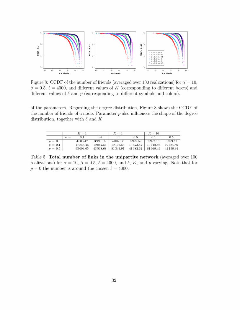
• the degree distribution, in the sense of the Complementary Cumulative Dis-tribution Function (CCDF) of the number of friends of each node (see Figure8).

The clustering coefficient C (and so the percentage of triangles) strongly in-creases with p (as expected). For p = 0 the percentage of closed triplets increases

30

with δ, but remains smaller or equal than 13% of total triplets for all consideredvalues of δ and K. For values of p greater than zero, the percentage of closed tripletsincreases with δ in a range of 13%−30% for p = 0.1 and in a range of 39%−62% forp = 0.5. The effect of K and δ seems to be marginal on the clustering coefficient.

δ = 0.1 0.15 0.2 0.25 0.3 0.35 0.4 0.45 0.5p = 0 0.04 0.05 0.07 0.08 0.08 0.10 0.13 0.13 0.10

K = 1 p = 0.1 0.13 0.17 0.20 0.23 0.23 0.24 0.26 0.27 0.30p = 0.5 0.39 0.45 0.45 0.49 0.49 0.47 0.49 0.53 0.62p = 0 0.06 0.06 0.08 0.09 0.08 0.11 0.13 0.13 0.11

K = 4 p = 0.1 0.15 0.18 0.21 0.24 0.23 0.25 0.26 0.28 0.30p = 0.5 0.42 0.47 0.46 0.49 0.49 0.48 0.50 0.53 0.62p = 0 0.06 0.06 0.08 0.09 0.08 0.11 0.13 0.14 0.11

K = 10 p = 0.1 0.15 0.18 0.21 0.24 0.23 0.25 0.26 0.28 0.30p = 0.5 0.42 0.47 0.46 0.49 0.49 0.48 0.49 0.53 0.62

Table 3: Clustering coefficient (averaged over 100 realizations) for α = 10, β =0.5, ℓ = 4000, and different values of δ, K, and p.

Looking at the values obtained for the fraction of pairs of nodes at distance atmost 20, for the two different values δ = 0.1 and δ = 0.5, we can notice a clear differ-ence in the behavior (independently of K and p): indeed, the fraction of reachablepairs for δ = 0.1 (when K and p are fixed) is highly greater than the correspondingfraction for δ = 0.5. Moreover, the fraction of reachable pairs decreases when Kincreases (and the other parameters are fixed) and slightly changes when only pvaries. The complementary fraction corresponds to the pairs of nodes at distancegreater than 20 or not reachable from each other.

The observed maximum distance h∗ (among pairs of nodes at distance at most20) varies in range of 2− 5 and decreases when δ (p and K, respectively) increasesand the other parameters are fixed.

K = 1 K = 4 K = 10δ = 0.1 0.5 0.1 0.5 0.1 0.5

p = 0 0.439 (5) 0.128 (4) 0.350 (4) 0.118 (4) 0.349 (4) 0.117 (4)p = 0.1 0.438 (4) 0.128 (3) 0.352 (3) 0.118 (3) 0.350 (3) 0.117 (3)p = 0.5 0.437 (3) 0.128 (2) 0.351 (2) 0.118 (2) 0.349 (2) 0.117 (2)

Table 4: Fraction of pairs of nodes at distance at most 20 (averaged over100 realizations) for α = 10, β = 0.5, ℓ = 4000, and different values of δ, K, andp. For each set of parameters, the corresponding observed maximum distance h∗ isreported in brackets.

Finally, the effect of p on the total number of links is clear: when p = 0 thenumber of links is approximately equal to the chosen ℓ (i.e. ℓ = 4000), since in thiscase we have only the first phase of the unipartite network construction: links arerelated only to the features. The larger p the more triplets are closed and so themore links we have. Table 5 reports the total number of links for all combinations

31

# of friends

CC

DF

− K

= 1

●●●●●●●●●●● ●● ●●● ●●●●●●● ●●●●●●●●●●●●●●●●●●●●●●●●●●●●●●●●●●●●●●●●●●●●●●●●●●●●●●●●●●●●●●●●●●●●●●●●●●●●●●●●●●●●●●●●●●●●●●●●●●●●●●●●●●●●●●●●●●●●●●●●●●●●●●●●●●●●●●●●●●●●●●●●●●●●●●●●●●●●●●●●●●●●●●●●●●●●●●●●●●●●●●●●●●●●●●●●●●●●●●●●●●●●●●●●●●●●●●●●●●●●●●●●●●●●●●●●●●●●●●●●●●●●●●●●●●●●●●●●●●●●●●●●●●●●●●●●●●●●●●●●●●●●●●●●●●●●●●●●●●●●●●●●●●●●●●●●●●●●●●●●●●●●●●●●●●●●●●●●●●●●●●●●●●●●●●●●●●●●●●●●●●●●●●●●●●●●●●●●●●●●●●●●●●●●●●●●●●●●●●●●●●●●●●●●●●●●●●●●●●●●●●●●●●●●●●●●●●●●●●●●●●●●●●●●●●●●●●●●●●●●●●●●●●●●●●●●●●●●●●●●●●●●●●●●●●●●●●●●●●●●●●●●●●●●●●●●●●●●●●●●●●●●●●●●●●●●●●●●●●●●●●●●●●●●●●●●●●●●●●●●●●●●●●●●●●●●●●●●●●●●●●●●●●●●●●●●●●●●●●●●●●●●●●●●●●●●●●●●●●●●●●●●●●●●●●●●●●●●●●●●●●●●●●●●●●●●●●●●●●●●●●●●●●●●●●●●●●●●●●●●●●●●●●●●●●●●●●●●●●●●●●●●●●●●●●●●●●●●●●●●●●●●●●●●●●●●●●●●●●●●●●●●●●●●●●●●●●●●●●●●●●●●●●●●●●●●●●●●●●●●●●●●●●●●●●●●●●●●●●●●●●●●●●●●●●●●●●●●●●●●●●●●●●●●●●●●●●●●●●●●●●●●●●●●●●●●●●●●●●●●●●●●●●●●●●●●●●●●●●●●●

●

●

●

●

●

●

10

−3

10

−2

10

−1

10

0

10−2

10−1

100

101

102

103

# of friends

CC

DF

− K

= 4

●●● ● ● ● ●●●●●●●●●●●●●●● ●●●●●●●●●●●●●●●●●●●●●●●●●●●●●●●●●●●●●●●●●●●●●●●●●●●●●●●●●●●●●●●●●●●●●●●●●●●●●●●●●●●●●●●●●●●●●●●●●●●●●●●●●●●●●●●●●●●●●●●●●●●●●●●●●●●●●●●●●●●●●●●●●●●●●●●●●●●●●●●●●●●●●●●●●●●●●●●●●●●●●●●●●●●●●●●●●●●●●●●●●●●●●●●●●●●●●●●●●●●●●●●●●●●●●●●●●●●●●●●●●●●●●●●●●●●●●●●●●●●●●●●●●●●●●●●●●●●●●●●●●●●●●●●●●●●●●●●●●●●●●●●●●●●●●●●●●●●●●●●●●●●●●●●●●●●●●●●●●●●●●●●●●●●●●●●●●●●●●●●●●●●●●●●●●●●●●●●●●●●●●●●●●●●●●●●●●●●●●●●●●●●●●●●●●●●●●●●●●●●●●●●●●●●●●●●●●●●●●●●●●●●●●●●●●●●●●●●●●●●●●●●●●●●●●●●●●●●●●●●●●●●●●●●●●●●●●●●●●●●●●●●●●●●●●●●●●●●●●●●●●●●●●●●●●●●●●●●●●●●●●●●●●●●●●●●●●●●●●●●●●●●●●●●●●●●●●●●●●●●●●●●●●●●●●●●●●●●●●●●●●●●●●●●●●●●●●●●●●●●●●●●●●●●●●●●●●●●●●●●●●●●●●●●●●●●●●●●●●●

●

●

●

●

●

●

10

−3

10

−2

10

−1

10

0

10−2

10−1

100

101

102

103

# of friends

CC

DF

− K

= 1

0

● ● ●●●●●● ●●●●●●●●●●●●●●●●●●●●●●●●●●●●●●●●●●●●●●●●●●●●●●●●●●●●●●●●●●●●●●●●●●●●●●●●●●●●●●●●●●●●●●●●●●●●●●●●●●●●●●●●●●●●●●●●●●●●●●●●●●●●●●●●●●●●●●●●●●●●●●●●●●●●●●●●●●●●●●●●●●●●●●●●●●●●●●●●●●●●●●●●●●●●●●●●●●●●●●●●●●●●●●●●●●●●●●●●●●●●●●●●●●●●●●●●●●●●●●●●●●●●●●●●●●●●●●●●●●●●●●●●●●●●●●●●●●●●●●●●●●●●●●●●●●●●●●●●●●●●●●●●●●●●●●●●●●●●●●●●●●●●●●●●●●●●●●●●●●●●●●●●●●●●●●●●●●●●●●●●●●●●●●●●●●●●●●●●●●●●●●●●●●●●●●●●●●●●●●●●●●●●●●●●●●●●●●●●●●●●●●●●●●●●●●●●●●●●●●●●●●●●●●●●●●●●●●●●●●●●●●●●●●●●●●●●●●●●●●●●●●●●●●●●●●●●●●●●●●●●●●●●●●●●●●●●●●●●●●●●●●●●●●●●●●●●●●●●●●●●●●●●●●●●●●●●●●●●●●●●●●●●●●●●●●●●●●●●●●●●●●●●●●●●●●●●●●●●●●●●●●●●●●●●●●●●●●●●●●●●●●●●●●●●●●●●●

●

●

●

●

●

●

10

−3

10

−2

10

−1

10

0

10−2

10−1

100

101

102

103

●

d = 0.1, p = 0

d = 0.1, p = 0.1

d = 0.1, p = 0.5

d = 0.5, p = 0

d = 0.5, p = 0.1

d = 0.5, p = 0.5

Figure 8: CCDF of the number of friends (averaged over 100 realizations) for α = 10,β = 0.5, ℓ = 4000, and different values of K (corresponding to different boxes) anddifferent values of δ and p (corresponding to different symbols and colors).

of the parameters. Regarding the degree distribution, Figure 8 shows the CCDF ofthe number of friends of a node. Parameter p also influences the shape of the degreedistribution, together with δ and K.

K = 1 K = 4 K = 10δ = 0.1 0.5 0.1 0.5 0.1 0.5

p = 0 4 003.47 3 998.15 4 002.17 3 999.59 3 997.13 3 999.52p = 0.1 17 853.46 19 862.54 19 107.53 19 523.42 19 112.46 19 484.86p = 0.5 93 093.05 43 538.68 81 343.97 41 382.62 81 039.49 41 156.34

Table 5: Total number of links in the unipartite network (averaged over 100realizations) for α = 10, β = 0.5, ℓ = 4000, and δ, K, and p varying. Note that forp = 0 the number is around the chosen ℓ = 4000.

32

2015 © IMT Institute for Advanced Studies, Lucca

Piazza San ponziano 6, 5100 Lucca, Italy. www.imtlucca.it