Homotopy theory for digraphs Alexander Grigor’yan * Department of Mathematics University of Bielefeld 33501 Bielefeld, Germany Yong Lin † Department of Mathematics Renmin University of China Beijing, China Yuri Muranov ‡ Department of Mathematics University of Warmia and Mazury Olsztyn, Poland Shing-Tung Yau § Department of Mathematics Harvard University Cambridge MA 02138, USA June 2014 Abstract We introduce a homotopy theory of digraphs (directed graphs) and prove its basic proper- ties, including the relations to the homology theory of digraphs constructed by the authors in previous papers. In particular, we prove the homotopy invariance of homologies of digraphs and the relation between the fundamental group of the digraph and its first homology group. The category of (undirected) graphs can be identified by a natural way with a full sub- category of digraphs. Thus we obtain also consistent homology and homotopy theories for graphs. Note that the homotopy theory for graphs coincides with the one constructed in [ 1] and [2]. Contents 1 Introduction 2 2 Homology theory of digraphs 3 2.1 The notion of a digraph ................................ 3 2.2 Paths and their boundaries .............................. 4 2.3 Regular paths ...................................... 4 2.4 Allowed and ∂ -invariant paths on digraphs ...................... 5 2.5 Cylinders ........................................ 7 3 Homotopy theory of digraphs 10 3.1 The notion of homotopy ................................ 10 3.2 Homotopy preserves homologies ............................ 11 * Partially supported by SFB 701 of German Research Council † Supported by the Fundamental Research Funds for the Central Universities and the Research Funds of (11XNI004) ‡ Partially supported by the CONACyT Grants 98697 and 151338, SFB 701 of German Research Council, and the travel grant of the Commission for Developing Countries of the International Mathematical Union § Partially supported by the grant ”Geometry and Topology of Complex Networks”, no. FA-9550-13-1-0097 1
Transcript
Homotopy theory for digraphs
Alexander Grigor’yan∗
Department of MathematicsUniversity of Bielefeld
33501 Bielefeld, Germany
Yong Lin†
Department of MathematicsRenmin University of China
Beijing, China
Yuri Muranov‡
Department of MathematicsUniversity of Warmia and Mazury
Olsztyn, Poland
Shing-Tung Yau §
Department of MathematicsHarvard University
Cambridge MA 02138, USA
June 2014
Abstract
We introduce a homotopy theory of digraphs (directed graphs) and prove its basic proper-ties, including the relations to the homology theory of digraphs constructed by the authors inprevious papers. In particular, we prove the homotopy invariance of homologies of digraphsand the relation between the fundamental group of the digraph and its first homology group.
The category of (undirected) graphs can be identified by a natural way with a full sub-category of digraphs. Thus we obtain also consistent homology and homotopy theories forgraphs. Note that the homotopy theory for graphs coincides with the one constructed in [1]and [2].
∗Partially supported by SFB 701 of German Research Council†Supported by the Fundamental Research Funds for the Central Universities and the Research Funds of
(11XNI004)‡Partially supported by the CONACyT Grants 98697 and 151338, SFB 701 of German Research Council, and
the travel grant of the Commission for Developing Countries of the International Mathematical Union§Partially supported by the grant ”Geometry and Topology of Complex Networks”, no. FA-9550-13-1-0097
The homology theory of digraphs has been constructed in a series of the previous papers of theauthors (see, for example, [5], [6], [7]). In the present paper we introduce a homotopy theoryof digraphs and prove that there are natural relations to aforementioned homology theory. Inparticular, we prove the invariance of the homology theory under homotopy and the relationbetween the fundamental group and the first homology group, which is similar to the one inthe classical algebraic topology. Let emphasize, that the theories of homology and homotopy ofdigraphs are introduced entirely independent each other, but nevertheless they exhibit a verytight connection similarly to the classical algebraic topology.
The homotopy theory of undirected graphs was constructed by Babson, Barcelo, Kramer,Laubenbacher, Longueville and Weaver in [1] and [2]. We identify in a natural way the categoryof graphs with a full subcategory of digraphs, which allows us to transfer the homology andhomotopy theories to undirected graphs. The homotopy theory of graphs, obtained in this way,coincides with the homotopy theory constructed in [1] and [2]. However, our notion of homologyof graphs is new, and the result about homotopy invariance of homologies of graphs is also new.Hence, our results give an answer to the question raised in [1] asking “for a homology theoryassociated to the A-theory of a graph”.
There are other homology theories on graphs that try to mimic the classical singular ho-mology theory. In those theories one uses predefined “small” graphs as basic cells and definessingular chains as formal sums of the maps of the basic cell into the graph (see, for example, [9],[13]). However, simple examples show that the homology groups obtained in this way, dependessentially on the choice of the basic cells.
Our homology theory of digraphs (and graphs) is very different from the ”singular” homologytheories. We do not use predefined cells but formulate only the desired properties of the cells interms of the digraph (graph) structure. Namely, each cell is determined by a sequence of verticesthat goes along the edges (allowed paths), and the boundary of the cell must also be of this type.This homology theory has very clear algebraic [6] and geometric [7], [5] motivation. It provideseffective computational methods for digraph (graph) homology, agrees with the homotopy theory,and provides good connections with homology theories of simplicial and cubical complexes [7]and, in particular, with homology of triangulated manifolds.
Let us briefly describe the structure of the paper and the main results. In Section 2 we givea short survey on homology theory for digraphs following [5], [7].
2
In Section 3, we introduce the notion of homotopy of digraphs. We prove the homotopyinvariance of homology groups (Theorem 3.3) and give a number of examples based on thenotion of deformation retraction.
In Section 4, we define a fundamental group π1 of digraph. Elements of π1 are equivalenceclasses of loops on digraphs, where the equivalence of the loops is defined using a new notion ofC-homotopy, which is more general than a homotopy. A description of C-homotopy in terms oflocal transformations of loops is given in Theorem 4.13.
We prove the homotopy invariance of π1 (Theorem 4.22) and the relation H1 = π1/ [π1, π1]between the first homology group over Z and the fundamental group (Theorem 4.23). We definehigher homotopy groups by induction using the notion of a loop digraph.
In Section 5 we give a new proof of the classical Sperner lemma, using fundamental groupsof digraphs. We hope that our notions of homotopy and homology theories on digraph can findfurther applications in graph theory, in particular, in graph coloring.
In Section 6 we construct isomorphism between the category of (undirected) graphs and afull subcategory of digraphs, thus transferring the aforementioned results from the category ofdigraphs to the category of graphs.
2 Homology theory of digraphs
In this Section we state the basic notions of homology theory for digraphs in the form that weneed in subsequent sections. This is a slight adaptation of a more general theory from [5], [7].
2.1 The notion of a digraph
We start with some definitions.
Definition 2.1 A directed graph (digraph) G = (V,E) is a couple of a set V , whose elementsare called the vertices, and a subset E ⊂ {V × V \ diag} of ordered pairs of vertices that arecalled (directed) edges or arrows. The fact that (v, w) ∈ E is also denoted by v → w.
In particular, a digraph has no edges v → v and, hence, it is a combinatorial digraph in thesense of [11]. We write
v−→=w
if either v = w or v → w. In this paper we consider only finite digraphs, that is, digraphs witha finite set of vertices.
Definition 2.2 A morphism from a digraph G = (VG, EG) to a digraph H = (VH , EH) is amap f : VG → VH such that for any edge v → w on G we have f (v)−→=f (w) on H (that is,either f(v) → f(w) or f(v) = f(w)). We will refer to such morphisms also as digraphs maps(sometimes simply maps) and denote them shortly by f : G→ H.
The set of all digraphs with digraphs maps form a category of digraphs that will be denotedby D.
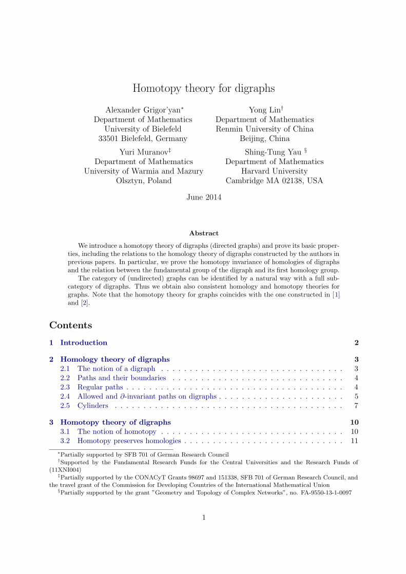
Definition 2.3 For two digraphs G = (VG, EG) and H = (VH , EH) define the Cartesian productG �H as a digraph with the set of vertices VG × VH and with the set of edges as follows: forx, x′ ∈ VG and y, y′ ∈ VH , we have (x, y)→ (x′, y′) in G�H if and only if
either x′ = x and y → y′, or x→ x′ and y = y′,
3
as is shown on the following diagram:
y′• . . .(x,y′)• −→
(x′,y′)• . . .
↑ ↑ ↑
y• . . .(x,y)• −→
(x′,y)• . . .
H � G . . . •x
−→ •x′
. . .
2.2 Paths and their boundaries
Let V be a finite set. For any p ≥ 0, an elementary p-path is any (ordered) sequence i0, ..., ip ofp+1 vertices of V that will be denoted simply by i0...ip or by ei0...ip . Fix a commutative ring Kwith unity and denote by Λp = Λp (V ) = Λp (V,K) the free K-module that consist of all formalK-linear combinations of all elementary p-paths. Hence, each p-path has a form
v =∑
i0i1...ip
vi0i1...ip ei0i1...ip , where vi0i1...ip ∈ K.
Definition 2.4 Define for any p ≥ 0 the boundary operator ∂ : Λp+1 → Λp by
(∂v)i0...ip =∑
k
p+1∑
q=0
(−1)q vi0...iq−1kiq ...ip (2.1)
where 1 is the unity of K and the index k is inserted so that it is preceded by q indices.
Sometimes we need also the operator ∂ : Λ0 → Λ−1 where we set Λ−1 = {0} and ∂v = 0 forall v ∈ Λ0. It follows from (2.1) that
∂ej0...jp+1 =p+1∑
q=0
(−1)q ej0...jq ...jp+1. (2.2)
It is easy to show that ∂2v = 0 for any v ∈ Λp ([5]). Hence, the family of K-modules{Λp}p≥−1 with the boundary operator ∂ determine a chain complex that will be denoted byΛ∗ (V ) = Λ∗ (V,K).
2.3 Regular paths
Definition 2.5 An elementary p-path ei0...ip on a set V is called regular if ik 6= ik+1 for allk = 0, ..., p − 1, and irregular otherwise.
Let Ip be the submodule of Λp that is K-spanned by irregular ei0...ip . It is easy to verifythat ∂Ip ⊂ Ip−1 (cf. [5]). Consider the quotient Rp := Λp/Ip. Since ∂Ip ⊂ Ip−1, the inducedboundary operator
∂ : Rp → Rp−1 (p ≥ 0)
is well-defined. We denote by R∗ (V ) the obtained chain complex. Clearly, Rp is linearlyisomorphic to the space of regular p-paths:
Rp∼= span K
{ei0...ip : i0...ip is regular
}(2.3)
4
For simplicity of notation, we will identify Rp with this space, by setting all irregular p-pathsto be equal to 0.
Given a map f : V → V ′ between two finite sets V and V ′, define for any p ≥ 0 the inducedmap
f∗ : Λp(V )→ Λp(V′)
by the rule f∗(ei0...ip
)= ef(i0)...f(ip), extended by K-linearity to all elements of Λp (V ). The
map f∗ is a morphism of chain complexes, because it trivially follows from (2.2) that ∂f∗ = f∗∂.Clearly, if ei0...ip is irregular then f∗
(ei0...ip
)is also irregular, so that
f∗ (Ip (V )) ⊂ Ip
(V ′) .
Therefore, f∗ is well-defined on the quotient Λp/Ip so that we obtain the induced map
f∗ : Rp (V )→ Rp
(V ′) . (2.4)
Since f∗ still commutes with ∂, we see that the induced map (2.4) induces a morphism R∗(V )→R∗(V ′) of chain complexes. With identification (2.3) of Rp we have the following rule for themap (2.4):
f∗(ei0...ip
)=
{ef(i0)...f(ip), if ef(i0)...f(ip) is regular,
0, if ef(i0)...f(ip) is irregular.(2.5)
2.4 Allowed and ∂-invariant paths on digraphs
Definition 2.6 Let G = (V,E) be a digraph. An elementary p-path i0...ip on V is calledallowed if ik → ik+1 for any k = 0, ..., p − 1, and non-allowed otherwise. The set of all allowedelementary p-paths will be denoted by Ep.
For example, E0 = V and E1 = E. Clearly, all allowed paths are regular. Denote byAp = Ap (G) the submodule of Rp (G) := Rp (V ) spanned by the allowed elementary p-paths,that is,
Ap = span K{ei0...ip : i0...ip ∈ Ep
}. (2.6)
The elements of Ap are called allowed p-paths.Note that the modules Ap of allowed paths are in general not invariant for ∂. Consider the
following submodules of Ap
Ωp ≡ Ωp (G) := {v ∈ Ap : ∂v ∈ Ap−1} (2.7)
that are ∂-invariant. Indeed, v ∈ Ωp implies ∂v ∈ Ap−1 and ∂ (∂v) = 0 ∈ Ap−2, whence∂v ∈ Ωp−1. The elements of Ωp are called ∂-invariant p-paths.
Hence, we obtain a chain complex Ω∗ = Ω∗ (G) = Ω∗ (G,K):
0 ← Ω0∂← Ω1
∂← . . .
∂← Ωp−1
∂← Ωp
∂← . . .
By construction we have Ω0 = A0 and Ω1 = A1, while in general Ωp ⊂ Ap.Let us define for any p ≥ 0 the homologies of the digraph G with coefficients from K by
Hp(G,K) = Hp (G) := Hp (Ω∗ (G)) = ker ∂|Ωp
/Im ∂|Ωp+1 .
Let us note that homology groups Hp (G) (as well as the modules Ωp (G)) can be computeddirectly by definition using simple tools of linear algebra, in particular, those implemented inmodern computational software. On the other hand, some theoretical tools for computation ofhomology groups like Kunneth formulas were developed in [5].
5
4
5
1
2
3
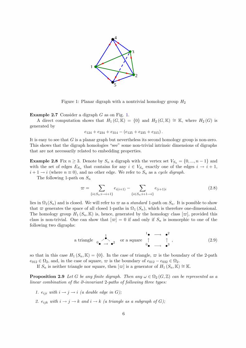
Figure 1: Planar digraph with a nontrivial homology group H2
Example 2.7 Consider a digraph G as on Fig. 1.A direct computation shows that H1 (G,K) = {0} and H2 (G,K) ∼= K, where H2 (G) is
It is easy to see that G is a planar graph but nevertheless its second homology group is non-zero.This shows that the digraph homologies “see” some non-trivial intrinsic dimensions of digraphsthat are not necessarily related to embedding properties.
Example 2.8 Fix n ≥ 3. Denote by Sn a digraph with the vertex set VSn = {0, ..., n − 1} andwith the set of edges ESn that contains for any i ∈ VSn exactly one of the edges i → i + 1,i + 1→ i (where n ≡ 0), and no other edge. We refer to Sn as a cycle digraph.
The following 1-path on Sn
$ =∑
{i∈Sn:i→i+1}
ei(i+1) −∑
{i∈Sn:i+1→i}
e(i+1)i (2.8)
lies in Ω1(Sn) and is closed. We will refer to $ as a standard 1-path on Sn. It is possible to showthat $ generates the space of all closed 1-paths in Ω1 (Sn), which is therefore one-dimensional.The homology group H1 (Sn,K) is, hence, generated by the homology class [$], provided thisclass is non-trivial. One can show that [$] = 0 if and only if Sn is isomorphic to one of thefollowing two digraphs:
a triangle ↗
1•↘
0• → •2or a square
1• −→ •2
↑ ↑0• −→ •3
, (2.9)
so that in this case H1 (Sn,K) = {0}. In the case of triangle, $ is the boundary of the 2-pathe012 ∈ Ω2, and, in the case of square, $ is the boundary of e012 − e032 ∈ Ω2.
If Sn is neither triangle nor square, then [$] is a generator of H1 (Sn,K) ∼= K.
Proposition 2.9 Let G be any finite digraph. Then any ω ∈ Ω2 (G,Z) can be represented as alinear combination of the ∂-invariant 2-paths of following three types:
1. eiji with i→ j → i (a double edge in G);
2. eijk with i→ j → k and i→ k (a triangle as a subgraph of G);
6
3. eijk − eimk with i→ j → k, i→ m→ k, i 6→ k, i 6= k (a square as a subgraph of G).
Proof. Since the 2-path ω is allowed, it can be represented as a sum of elementary 2-patheijk with i→ j → k multiplied with +1 or −1. If k = i then eijk is a double edge. If i 6= k andi→ k then eijk is a triangle. Subtracting from ω all double edges and triangles, we can assumethat ω has no such terms any more. Then, for any term eijk in ω we have i 6= k and i 6→ k. Fixsuch a pair i, k and consider any vertex j with i→ j → k. The 1-path ∂ω is the sum of 1-pathsof the form
∂eijk = eij − eik + ejk.
Since ∂ω is allowed but eik is not allowed, the term eik should cancel out after we sum up allsuch terms over all possible j. Therefore, the number of j such that eijk enters ω with coefficient+1 is equal to the number of j such that eijk enters in ω with the coefficient −1. Combiningthe pair with +1 and −1 together, we obtain that ω is the sum of the terms of the third type(squares).
Theorem 2.10 Let G and G′ be two digraphs, and f : G → G′ be a digraph map. Then themap f∗|Ωp(G) (where f∗ is the induced map (2.4)) provides a morphism of chain complexes
Ω∗(G,K)→ Ω∗(G′,K)
and, consequently, a homomorphism of homology groups
H∗(G,K)→ H∗(G′,K)
that will also be denoted by f∗.
Proof. By construction Ωp (G) is a submodule of Rp (G), and all we need to prove is that
f∗ (Ωp (G)) ⊂ Ωp
(G′) . (2.10)
Let us first show thatf∗ (Ap (G)) ⊂ Ap
(G′) .
It suffices to prove that if ei0...ip is allowed on G then f∗(ei0...ip
)is allowed on G′. Indeed, if
ef(i0)...(ip) is irregular then we have by (2.5) that f∗(ei0...ip
)= 0 ∈ Ap (G′) . If ef(i0)...(ip) is regular
then f (ik) 6= f (ik+1) for all k = 0, ..., p−1. Since ik → ik+1 on G, by the definition of a digraphmap we have either f (ik) → f (ik+1) on G′ or f (ik) = f (ik+1). Since the second possibility isexcluded, we obtain f (ik)→ f (ik+1) for all k, whence it follows that f∗
(ei0...ip
)= ef(i0)...(ip) is
allowed on G′.Now we can prove (2.10). For any v ∈ Ωp (G) we have by (2.7) v ∈ Ap (G) and ∂v ∈ Ap−1 (G),
whencef∗ (v) ∈ Ap
(G′) and ∂ (f∗ (v)) = f∗ (∂v) ∈ Ap−1
(G′) ,
which implies f∗ (v) ∈ Ωp (G′) .
2.5 Cylinders
For any digraph G consider its product G � I with the digraph I =(0• → •1
)(see Definition
2.3).
Definition 2.11 The digraph G� I is called the cylinder over G and will be denoted by Cyl Gor by G.
7
By the definition of Cartesian product, the set of vertices of G is V = V ×{0, 1}, and the setE of its edges is defined by the rule: (x, a) → (y, b) if and only if either x → y in G and a = bor x = y and a → b in I. We shall put the hatover all notation related to G, for example,Rp := Rp(G) and Ωp := Ωp(G). One can identify V = V × {0, 1} with V t V ′ where V ′ is acopy of V , and use the notation (x, 0) ≡ x and (x, 1) ≡ x′.
Define the operation of lifting paths from G to G as follows. If v = ei0...ip then v is a
(p + 1)-path in G defined by
v =p∑
k=0
(−1)k ei0...iki′k...i′p. (2.11)
By K-linearity this definition extends to all v ∈ Rp, thus giving v ∈ Rp+1. It follows that, forany v ∈ Rp and any path i0...ip on G,
vi0...iki′k...i′p = (−1)k vi0...ip . (2.12)
Clearly, i0...ip is allowed in G if and only if i0...iki′k...i
′p is allowed in G:
∙ ∙ ∙i′k• −→
i′k+1• −→ ∙ ∙ ∙ −→
i′p•
↑ ↑i0• −→ ∙ ∙ ∙ −→
ik• −→ik+1• ∙ ∙ ∙
,
for some/all k. Hence, we see that v ∈ Ap if and only if v ∈ Ap+1.
Proposition 2.12 If v ∈ Ωp then v ∈ Ωp+1.
Proof. We need to prove that if v ∈ Ap and ∂v ∈ Ap−1 then ∂v ∈ Ap. Let us prove firstsome properties of the lifting. For any path v in G define its image v′ in G′ = (V ′, E′) by
(ei0...ip
)′ = ei′0...i′p.
Let us show first that, for any p-path u and q-path v on G, the following identity holds:
uv = uv′ + (−1)p+1 uv. (2.13)
It suffices to prove it for u = ei0...ip and v = ej0...jq . Then uv = ei0...ipj0...jq and
uv =p∑
k=0
(−1)k ei0...iki′k...i′pj′0...j′q+
q∑
k=0
(−1)k+p+1 ei0...ipj0...jkj′k...j′q
= uv′ + (−1)p+1 uv.
Now let us show that, for any p-path v with p ≥ 0
∂v = −∂v + v′ − v. (2.14)
It suffices to prove it for v = ei0...ip , which will be done by induction in p. For p = 0 write v = ea
so that ∂v = 0 and v = eaa′ whence
∂v = ea′ − ea = −∂v + v′ − v.
8
For p > 1 write v = ueip where u = ei0...ip−1 . Using (2.13) and the inductive hypothesis withthe (p− 1)-path u we obtain
= (−∂u + u′ − u)ei′p + (−1)p+1 u + (−1)p (∂u) eipi′p + uei′p − v
= −(∂u)ei′p + v′ + (−1)p+1 u + (−1)p (∂u) eipi′p − v .
On the other hand,
∂v =((∂u) eip + (−1)p u
)ˆ = (∂u)ei′p + (−1)p−1 (∂u) eipi′p + (−1)p u,
whence it follows that ∂v + ∂v = v′ − v, which finishes the proof of (2.14).Finally, if v ∈ Ap and ∂v ∈ Ap−1 then v′ and ∂v belong to Ap whence it follows from (2.14)
also ∂v ∈ Ap. This proves that v ∈ Ap+1.
Example 2.13 The cylinder over the digraph 0• → •1 is a square
2• −→ •3
↑ ↑0• −→ •1
Lifting a ∂-invariant 1-path e01 ∈ Ω1 we obtain a ∂-invariant 2-path on the square: e00′1′−e011′ ,that can be rewritten in the form e023 − e013.
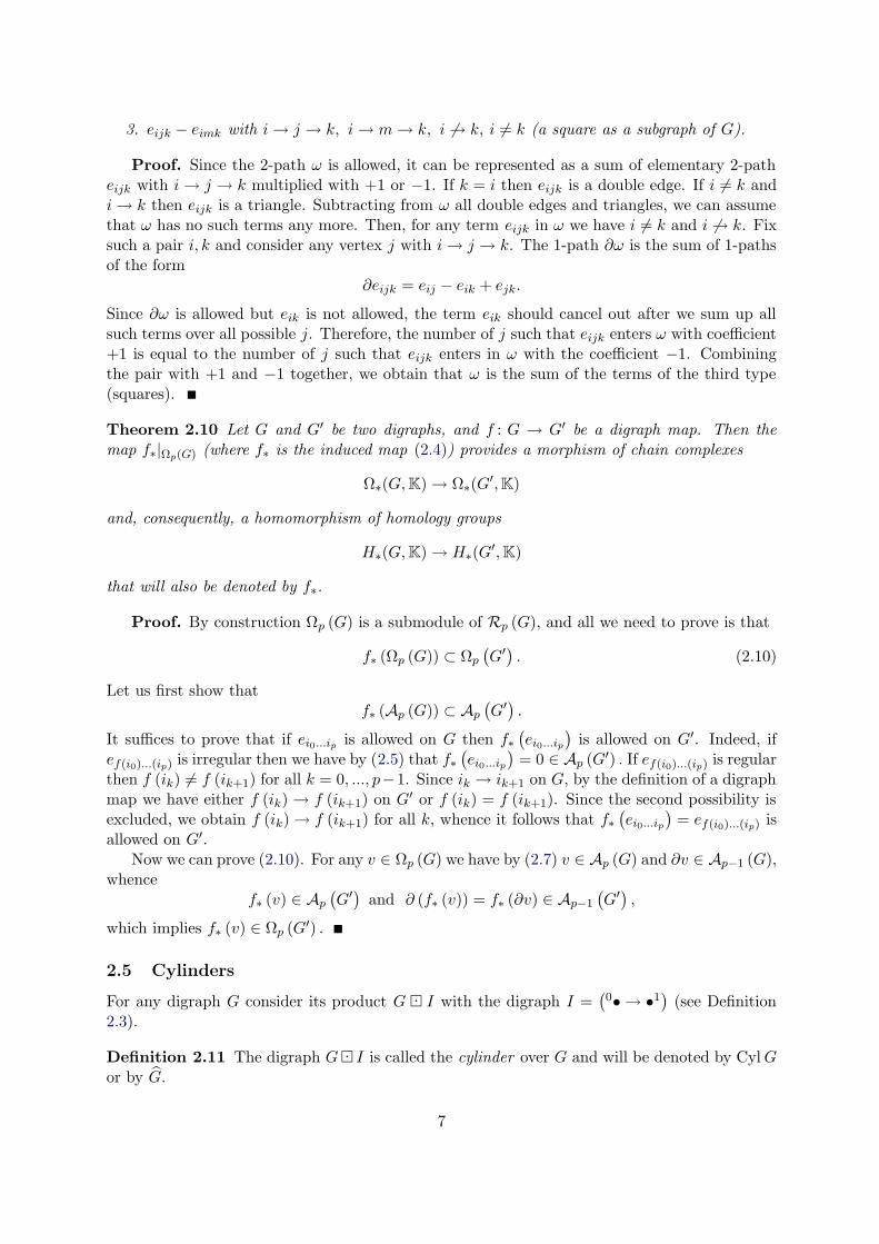
The cylinder over a square is a 3-cube that is shown in Fig. 2.
0 1
3 2
4 5
7 6
Figure 2: 3-cube
Lifting the 2-path e023 − e013 we obtain a ∂-invariant 3-path on the 3-cube:
e0467 − e0267 + e0237 − e0457 + e0157 − e0137.
Defining further n-cube as the cylinder over (n− 1)-cube, we see that n-cube determines a ∂-invariant n-path that is a lifting of a ∂-invariant (n− 1)-path from (n− 1)-cube and that is analternating sum of n! elementary terms. One can show that this n-path generates Ωn on n-cube(see [7]).
9
3 Homotopy theory of digraphs
In this Section we introduce a homotopy theory of digraphs and establish the relations betweenthis theory and the homology theory of digraphs of [5] and [7].
3.1 The notion of homotopy
Fix n ≥ 0. Denote by In any digraph whose the set of vertices is {0, 1, . . . , n} and the set ofedges contains exactly one of the edges i → (i + 1), (i + 1) → i for any i = 0, 1, . . . , n − 1, andno other edges. A digraph In is called a line digraph. Denote by In the set of all line digraphsIn and by I the union of all In.
Clearly, there is only one digraph in I0 – the one-point digraph. There are two digraphs inI1: the digraph I with the edge (0→ 1) and the digraph I− with the edge (1→ 0).
Definition 3.1 Let G,H be two digraphs. Two digraph maps f, g : G→ H are called homotopicif there exists a line digraph In ∈ In with n ≥ 1 and a digraph map
F : G� In → H
such thatF |G�{0} = f and F |G�{n} = g. (3.1)
In this case we shall write f ' g. The map F is called a homotopy between f and g.
In the case n = 1 we refer to the map F as an one-step homotopy between f and g. In thiscase the identities (3.1) determine F uniquely, and the requirement is that the so defined F isa digraph map of G � I1 to H. Since for I1 there are only two choices 0 → 1 and 0 ← 1, weobtain that f and g are one-step homotopic, if
either f (x)−→=g (x) for all x ∈ VG or g (x)−→=f (x) for all x ∈ VG. (3.2)
It follows that f and g are homotopic if there is a finite sequence of digraph maps f =f0, f1, ..., fn = g from G to H such that fk and fk+1 are one-step homotopic. It is obviousthat the relation ”'” is an equivalence relation on the set of all digraph maps from G to H.
Definition 3.2 Two digraphs G and H are called homotopy equivalent if there exist digraphmaps
f : G→ H, g : H → G (3.3)
such thatf ◦ g ' idH , g ◦ f ' idG . (3.4)
In this case we shall write H ' G. The maps f and g as in (3.4) are called homotopy inversesof each other.
A digraph G is called contractible if G ' {∗} where {∗} is a single vertex digraph. Itfollows from Definition 3.2 that a digraph G is contractible if and only if there is a digraphmap h : G → G such that the image of h consists of a single vertex and h ' idG . Examples ofcontractible digraphs will be given in Section 3.3.
10
3.2 Homotopy preserves homologies
Now we can prove the first result about connections between homotopy and homology theoriesfor digraphs.
Theorem 3.3 Let G,H be two digraphs.
(i) Let f ' g : G→ H be two homotopic digraph maps. Then these maps induce the identicalhomomorphisms of homology groups of G and H, that is, the maps
f∗ : Hp (G)→ Hp (H) and g∗ : Hp (G)→ Hp (H)
are identical.
(ii) If the digraphs G and H are homotopy equivalent, then they have isomorphic homologygroups. Furthermore, if the homotopical equivalence of G and H is provided by the digraphmaps (3.3) then their induced maps f∗ and g∗ provide mutually inverse isomorphisms ofthe homology groups of G and H.
In particular, if a digraph G is contractible, then all the homology groups of G are trivial,except for H0.
Proof. (i) Let F be a homotopy between f and g as in Definition 3.1. Consider first thecase n = 1 and let In be the digraph I = (0→ 1) (the case In = I− is similar). The maps f andg induce morphisms of chain complexes
f∗, g∗ : Ω∗(G)→ Ω∗(H),
and F induces a morphismF∗ : Ω∗(G� I)→ Ω∗(H).
Note that, for any path v ∈ Ω∗(G� I) that lies in G� {0}, we have F∗ (v) = f∗ (v), and for anypath v′ ∈ Ω∗(G� I) that lies in G� {1}, we have F∗ (v′) = g (v′) .
In order to prove that f∗ and g∗ induce the identical homomorphisms H∗ (G) → H∗ (H), itsuffices by [10, Theorem 2.1, p.40] to construct a chain homotopy between the chain complexesΩ∗ (G) and Ω∗ (H), that is, the K-linear mappings
Lp : Ωp(G)→ Ωp+1(H)
such that∂Lp + Lp−1∂ = g∗ − f∗
(note that all the terms here are mapping from Ωp (G) to Ωp (H)). Let us define the mappingLp as follows
Lp(v) = F∗ (v) ,
for any v ∈ Ωp (G), where v ∈ Ωp+1 (G� I) is lifting of v to the graph G = G � I defined inSection 2.5. Using ∂F∗ = F∗∂ (see Theorem 2.10) and the product rule (2.14), we obtain
(∂Lp + Lp−1∂)(v) = ∂(F∗(v)) + F∗(∂v)
= F∗ (∂v) + F∗(∂v)
= F∗(∂v + ∂v)
= F∗(v′ − v
)
= g∗ (v)− f∗ (v) .
11
The case of an arbitrary n follows then by induction.(ii) Let f, g be the maps from Definition 3.2. Then they induce the following mappings
Hp (G)f∗→ Hp (H)
g∗→ Hp (G)f∗→ Hp (H) .
By (i) and (3.4) we have f∗ ◦ g∗ = id and g∗ ◦ f∗ = id, which implies that f∗ and g∗ are mutuallyinverse isomorphisms of Hp (G) and Hp (H).
3.3 Retraction
A (induced) sub-digraph H of a digraph G is a digraph whose set of vertices is a subset of thatof G and the edges of H are all those edges of G whose adjacent vertices belong to H.
Definition 3.4 Let G be a digraph and H be its sub-digraph.(i) A retraction of G onto H is a digraph map r : G→ H such that r|H = idH .(ii) A retraction r : G→ H is called a deformation retraction if i◦ r ' idG, where i : H → G
is the natural inclusion map.
Proposition 3.5 Let r : G → H be a deformation retraction. Then G ' H and the maps r, iare homotopy inverses.
Proof. By definition of retraction we have r ◦ i = IdH and, in particular r ◦ i ' idH . Sincei ◦ r ' idG, we obtain by Definition 3.2 that G ' H.
In general the existence of a deformation retraction r : G → H is a stronger condition thatthe homotopy equivalence G ' H. However, in the case when H = {∗}, the existence of adeformation retraction r : G→ {∗} is equivalent to the contractibility of G, which follows fromthe remark after Definition 3.2.
The next two statements provide a convenient way of constructing a deformation retraction.
Proposition 3.6 Let r : G→ H be a retraction of a digraph G onto a sub-digraph H. Assumethat there exists a finite sequence {fk}
nk=0 of digraph maps fk : G → G with the following
properties:
1. f0 = idG;
2. fn = i ◦ r (where i is the inclusion map i : H → G), that is, fn (v) = r (v) for all verticesv of G;
3. for any k = 1, ..., n either fk−1 (x)−→=fk (x) for all x ∈ VG or fk (x)−→=fk−1 (x) for allx ∈ VG.
Then r is a deformation retraction, the digraphs G and H are homotopy equivalent, and i,r are their homotopy inverses.
Proof. Since fk−1 and fk satisfy (3.2), we see that fk−1 ' fk whence by induction we obtainthat fn ' f0 and, hence, i◦r ' idG . Therefore, r is a deformation retraction, and the rest followfrom Proposition 3.4.
Corollary 3.7 Let r : G→ H be a retraction of a digraph G onto a sub-digraph H and
x−→=r (x) for all x ∈ VG or r (x) −→=x for all x ∈ VG. (3.5)
Then r is a deformation retraction, the digraphs G and H are homotopy equivalent, and i, r aretheir homotopy inverses.
12
Clearly, Corollary 3.7 is an important particular case n = 1 of Proposition 3.6. Note alsothat the condition (3.5) is automatically satisfies for all x ∈ VH , so in applications it remains toverify it for v ∈ VG \ VH .
Corollary 3.8 For any digraph G and for any line digraph In ∈ In (n ≥ 0) we have G�In ' G.
Proof. It suffices to show that G � In ' G � In−1 where In−1 is obtained from In byremoving the vertex n and the adjacent edge, and then to argue by induction since G� I0 = G.Define a retraction r : G� In → G� In−1 by
r (x, k) =
{(x, k) , k ≤ n− 1,(x, n− 1) , k = n.
Let us show that r is an 1-step deformation retraction, that is, r satisfied (3.5):
(x, k) −→=r (x, k) for all (x, k) ∈ G� In or r (x, k) −→= (x, k) for all (x, k) ∈ G� In
Indeed, for k ≤ n− 1 this is obvious. If k = n then consider two cases.
1. If (n− 1)→ n in In then (x, n− 1)→ (x, n) in G� In whence
r (x, k) = r (x, n) = (x, n− 1)→ (x, n) = (x, k) .
2. If n→ (n− 1) in In then (x, n)→ (x, n− 1) in G� In whence
(x, k)→ r (x, k) .
Corollary 3.9 Let G be a digraph. Fix some n ∈ N and consider for any k = 0, ..., n the naturalinclusion
ik : G→ G� In, ik(v) = (v, k)
and a natural projectionp : G� In → G, p(v, k) = v.
Then the maps i,p induce isomorphism of homology groups.
Proof. The projection p can be decomposed into composition of retractions G � Im →G � Im−1 which are homotopy equivalences by the proof of Corollary 3.8. Therefore, p is alsoa homotopy equivalence and hence induces isomorphism of homology groups. The inclusion ikcan be decomposed into composition of natural inclusions G � Im−1 → G � Im, each of thembeing homotopy inverse of the retraction G� Im → G� Im−1, which implies the claim.
Example 3.10 A digraph G is called a tree if the underlying undirected graph is a tree. Weclaim that if a digraph G is a connected tree then G is contractible. Indeed, let a be a pendantvertex of G and let b be another vertex such that a → b or b ← a. Let G′ be the subgraphof G that is obtained from G by removing the vertex a with the adjacent edge. Then the mapr : G → G′ defined by r (a) = b and r|H = id is by Corollary 3.7 a deformation retraction,whence G ' G′. Since G′ is also a connected tree, continuing the procedure of removing of apendant vertices, we obtain in the end that G is contractible.
13
0
3
1
2
0
3
1
2
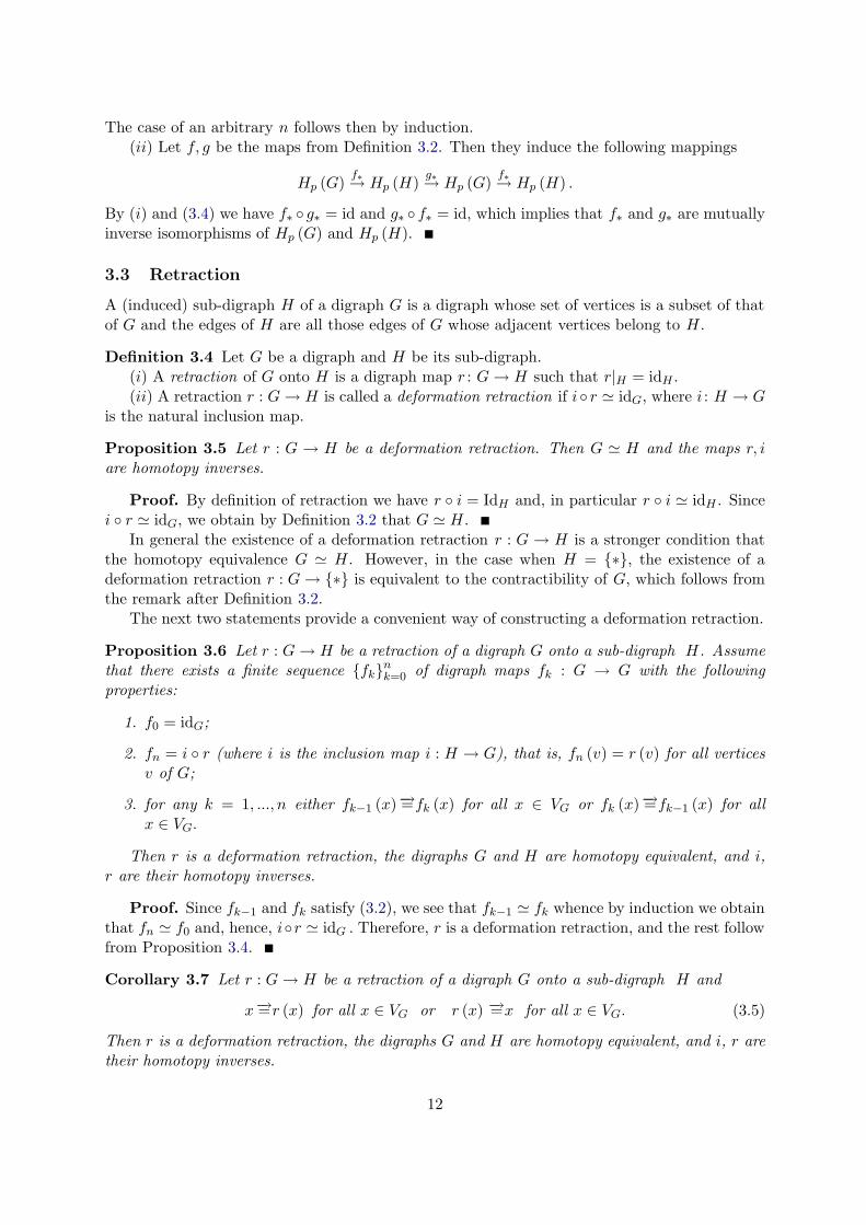
Figure 3: Star-like digraphs
Example 3.11 A digraph G is called star-like (resp. inverse star-like) if there is a vertexa ∈ VG such that a → x (resp. x → a) for all x ∈ VG \ {a} . if G is a (inverse) star-likedigraph, then the map r : G → {a} is by Corollary 3.7 a deformation retraction, whence weobtain G ' {a}, that is, G is contractible. Consequently, all homology groups of G are trivialexcept for H0.
For example, consider a digraph-simplex of dimension n, which is a digraph G with the setof vertices {0, 1, . . . , n} and the set of edges given by the condition
i→ j ⇐⇒ i < j
(a digraph-simplex with n = 3 is shown on the left panel on Fig. 3). Then G is star-like and,hence, G is contractible. In particular, the triangular digraph from Example 2.8 is contractible.Another star-like digraph is shown on the right panel of Fig. 3.
Example 3.12 For any n ≥ 1, consider the n-dimensional cube
In = I � I � ∙ ∙ ∙� I︸ ︷︷ ︸n times
For example, I2 is the square from Example 2.8 and I3 is a 3-cube shown on Fig. 2. ByCorollary 3.8 we have Ik ' Ik−1, whence we obtain that, for all n, In ' I, which implies that In
is contractible. In particular, this applies to a square digraph from Example 2.8. Consequently,the all homology groups of In are trivial except for H0.
Example 3.13 Let Sn be a cycle digraph from Example 2.8. If Sn is the triangle or squareas in (2.9) then Sn is contractible as was shown in Examples 3.11 and 3.12, respectively. IfSn is neither triangle nor square then by Example 2.8 H1(Sn,K) ∼= K and, hence, Sn is notcontractible. In particular, this is always the case when n ≥ 5. Here are other examples ofnon-contractible cycles with n = 3, 4:
↗
1•↘
0• ←− •2and
1• −→ •2
↑ ↓0• ←− •3
,
Let us show that two cycles Sn and Sm with n 6= m are not homotopy equivalent, except forthe case when one of them is a triangle and the other is a square. Assume that Sn and Sm withn < m are homotopy equivalent. Then by Theorem 3.3 there is a digraph map f : Sn → Sm
such that f∗ : H1 (Sn)→ H1 (Sm) is an isomorphism. If homology groups H1 (Sn) and H1 (Sm)
14
0
3
4
2
1
Figure 4: The digraph admits a deformation retraction onto a subgraph {1, 3, 4}
are not isomorphic then we are done. If they are isomorphic, then they are isomorphic to K.Let $n ∈ Ω1 (Sn) be the generator of closed 1-paths on Sn and $m ∈ Ω1 (Sm) be the generatorof closed 1-paths on Sn, as in (2.8). Then [$n] generates H1 (Sn), [$m] generates H1 (Sm), andwe should have
f∗ ([$n]) = k [$m]
for some non-zero constant k ∈ K. Consequently, we obtain
f∗ ($n) = k$m,
which is impossible because f cannot be surjective by n < m, whereas $m uses all the verticesof Sm.
Example 3.14 Consider the digraph G as on Fig. 4.Consider also its sub-digraph H with the vertex set VH = {1, 3, 4} and a retraction r : G→ H
given by r (0) = 1, r (2) = 3 and r|H = id. By Corollary 3.7, r is a deformation retraction,whence G ' H. Consequently, we obtain H1 (G,K) ∼= H1 (H,K) ∼= K and Hp (G,K) = {0} forp ≥ 2.
Example 3.15 Let a be a vertex in a digraph G and let b0, b1, ..., bn be all the neighboringvertices of a in G. Assume that the following condition is satisfied:
∀i = 1, ..., n a→ bi ⇒ b0 → bi and a← bi ⇒ b0 ← bi. (3.6)
Denote by H the digraph that is obtained from G by removing a vertex a with all adjacentedges. The map r : G → H given by r (a) = b0 and r|H = id is by Corollary 3.7 a deformationretraction, whence we obtain that G ' H. Consequently, all homology groups of G and H arethe same. This is very similar to the results about transformations of simplicial complexes inthe simple homotopy theory (see, for example, [3]).
In particular, (3.6) is satisfied if a → bi and b0 → bi for all i ≥ 1 or a ← bi and b0 ← bi forall i ≥ 1. Two examples when (3.6) is satisfied are shown in the following diagram:
↗a • −→
↘
• b1
↑• b0
↓• b1
∙ ∙ ∙ H G↗
a • ←−↖
• b1
↑• b0
↑• b1
∙ ∙ ∙ H G
15
4
5
1
2
3
4
5
1
2
3
Figure 5: The left digraph is contractible while the right one is not.
On the contrary, the digraph G on following diagram
• b1
↗ ↓a • ←− • b0
does not satisfy (3.6). Moreover, this digraph is not homotopy equivalent to H =(0• → •1
)
since G and H have different homology group H1 (cf. Example 2.8).For example, the digraph on the left panel of Fig. 5 is contractible as one can successively
remove the vertices 5, 4, 3, 2 each time satisfying (3.6).The digraph on the right panel of Fig. 5 is different from the left one only by the direction
of the edge between 1 and 3, but it is not contractible as its H2 group is non-trivial by Example2.7.
Consider one more example: the digraph G on Fig. 6.
3
6
2
5 4
1
7
0
9
8 A
B
Figure 6: Digraph G whose H2 group is generated by an octahedron
Removing successively the vertices A,B, 8, 9, 6, 7, which each time satisfy (3.6), we obtain adigraph H with VH = {0, 1, 2, 3, 4, 5} that is homotopy equivalent to G and, in particular, hasthe same homologies as G. The digraph H is shown in two ways on Fig. 7. Clearly, the secondrepresentation of this graph is reminiscent of an octahedron.
16
3
2
5 4
1
0
= 1
0
4
5
2
3
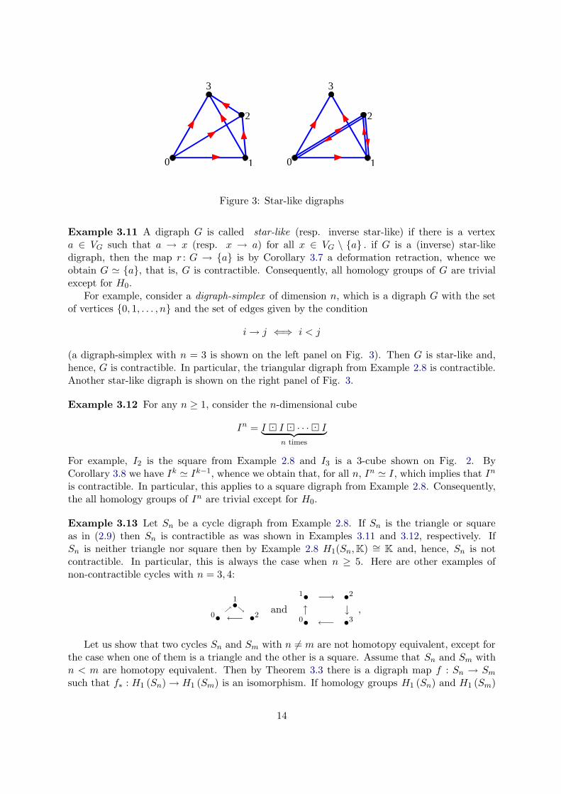
Figure 7: Two representations of the digraph H
It is possible to show that Hp (H,K) = {0} for p = 1 and p > 2 while H2 (H,K) ∼= K. Itfollows that the same is true for the homology groups of G. Furthermore, it is possible to showthat H2 (G,K) is generated by the following 2-path
that determines a 2-dimensional “hole” in G given by the octahedron H. Note that on Fig. 6this octahedron is hardy visible.
3.4 Cylinder of a map
Let us give some further examples of homotopy equivalent digraphs.
Definition 3.16 Let G = (VG, EG) and H = (VH , EH) be two digraphs and f be a digraphmap from G to H. The cylinder Cf of f is the digraph with the set of vertices VCf
= VG t VH
and with the set of edges ECfthat consists of all the edges from EG and EH as well as of the
edges of the form x→ f (x) for all x ∈ VG.The inverse cylinder C−
f is defined in the same way except that the edge x→ f (x) is replacedby f (x)→ x.
For example, for f = idG we have Cf = G � I where I =(0• −→ •1
)and C−
f = G � I−
where I− =(0• ←− •1
).
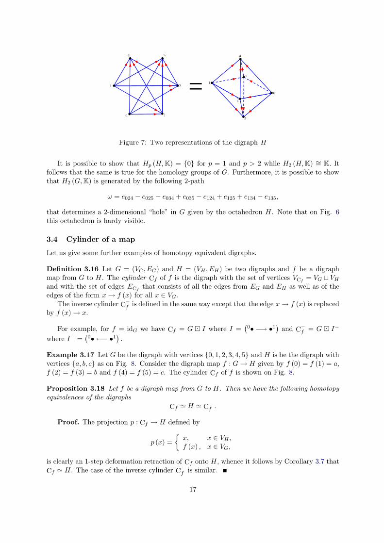
Example 3.17 Let G be the digraph with vertices {0, 1, 2, 3, 4, 5} and H is be the digraph withvertices {a, b, c} as on Fig. 8. Consider the digraph map f : G→ H given by f (0) = f (1) = a,f (2) = f (3) = b and f (4) = f (5) = c. The cylinder Cf of f is shown on Fig. 8.
Proposition 3.18 Let f be a digraph map from G to H. Then we have the following homotopyequivalences of the digraphs
Cf ' H ' C−f .
Proof. The projection p : Cf → H defined by
p (x) =
{x, x ∈ VH ,f (x) , x ∈ VG,
is clearly an 1-step deformation retraction of Cf onto H, whence it follows by Corollary 3.7 thatCf ' H. The case of the inverse cylinder C−
f is similar.
17
1 2
3
4
5
0
a b
c
Figure 8: The cylinder of the map
4 Homotopy groups of digraphs
In this Section we define homotopy groups of digraphs and describe theirs basic properties. Forthat, we introduce the concept of path-map in a digraph G, and then define a fundamentalgroup of G. Then the higher homotopy group can be defined inductively as the fundamentalgroup of the corresponding iterated loop-digraph.
A based digraph G∗ is a digraph G with a fixed base vertex ∗ ∈ VG. A based digraph mapf : G∗ → H∗ is a digraph map f : G → H such that f (∗) = ∗. A category of based digraphswill be denoted by D∗.
A homotopy between two based digraph maps f, g : G∗ → H∗ is defined as in Definition 3.1with additional requirement that F |{∗}�In
= ∗.
4.1 Construction of π0
Let G∗ be a based digraph, and V ∗2 = {0, 1} be the based digraph consisting of two vertices,
no edges and with the base vertex 0 = ∗. Let Hom(V ∗2 , G∗) be the set of based digraph maps
from V ∗2 to G∗. Note that the set of such maps is in one to one correspondence with the set of
vertices of the digraph G.
Definition 4.1 We say that two digraph maps φ, ψ ∈ Hom(V ∗2 , G∗) are equivalent and write
φ ' ψ if there exists In ∈ I and a digraph map
f : In → G,
such that f(0) = φ (1) and f(n) = ψ (1). The relation ' is evidently an equivalence relation,and we denote by [φ] the equivalence class of the element φ, and by π0(G∗) the set of classes ofequivalence with the base point ∗ given by a class of equivalence of the trivial map V2 → ∗ ∈ G.
The set π0(G∗) coincides with the set of connected components of the digraph G. In partic-ular, the digraph G∗ connected if π0(G∗) = ∗.
Proposition 4.2 Any based digraph map f : G∗ → H∗ induces a map
π0(f) : π0(G∗)→ π0(H
∗)
of based sets. The homotopic maps induce the same map of based sets. We have a functor fromthe category D∗ of digraphs to the category based sets.
Proof. Let x = [φ] ∈ π0(G∗) be presented by a digraph map φ : V ∗2 → G∗ we put y =
[π0(f)](x) = [f ◦φ] ∈ π0(H∗). It is an easy exercise to check that this map π0(f) is well definedand for the homotopic maps f ' g : G∗ → H∗ we have π0(f) = π0(g).
18
4.2 C-homotopy and π1
For any line digraph In ∈ In, a based digraph I∗n will always have the base point 0.
Definition 4.3 A path-map in a digraph G is any digraph map φ : In → G, where In ∈ In. Abased path-map on a based digraph G∗ is a based digraph map φ : I∗n → G∗, that is, a digraphmap such that φ (0) = ∗. A loop on G∗ is a based path-map φ : I∗n → G∗ such that φ (n) = ∗.
Note that the image of a path-map is not necessary an allowed path of the digraph G.
Definition 4.4 A digraph map h : In → Im is called shrinking if h (0) = 0, h(n) = m, andh (i) ≤ h (j) whenever i ≤ j (that is, if h as a function from {0, ..., n} to {0, ...,m} is monotoneincreasing).
Any shrinking h : In → Im is by definition a based digraph map. Moreover, h is surjectiveand the preimage of any edge of Im consists of exactly one edge of In. Furthermore, we havenecessarily m ≤ n, and if n = m then h is a bijection.
Definition 4.5 Consider two based path-maps
φ : I∗n → G∗ and ψ : I∗m → G∗.
An one-step direct C-homotopy from φ to ψ is given by a shrinking map h : In → Im such thatthe map F : VCh
→ VG given by
F |In = φ and F |Im = ψ, (4.1)
is a digraph map from Ch to G. If the same is true with Ch replaced everywhere by C−h then
we refer to an one-step inverse C-homotopy.
Remark 4.6 The requirement that F is a digraph map is equivalent to the condition
φ (i)−→=ψ (h (i)) for all i ∈ In. (4.2)
In turn, (4.2) implies that the digraph maps φ and ψ ◦ h (acting from In to G) satisfy (3.2),which yields φ ' ψ ◦ h.
If n = m then h = idIn and an one-step C-homotopy is a homotopy.
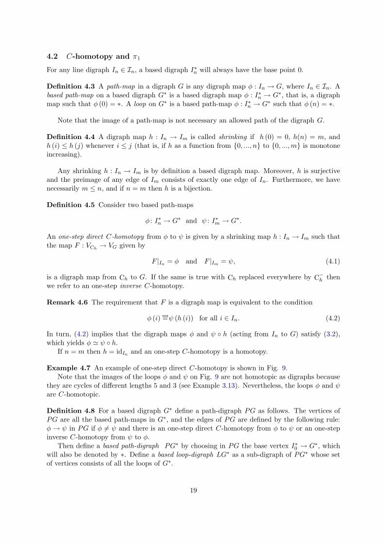
Example 4.7 An example of one-step direct C-homotopy is shown in Fig. 9.Note that the images of the loops φ and ψ on Fig. 9 are not homotopic as digraphs because
they are cycles of different lengths 5 and 3 (see Example 3.13). Nevertheless, the loops φ and ψare C-homotopic.
Definition 4.8 For a based digraph G∗ define a path-digraph PG as follows. The vertices ofPG are all the based path-maps in G∗, and the edges of PG are defined by the following rule:φ→ ψ in PG if φ 6= ψ and there is an one-step direct C-homotopy from φ to ψ or an one-stepinverse C-homotopy from ψ to φ.
Then define a based path-digraph PG∗ by choosing in PG the base vertex I∗0 → G∗, whichwill also be denoted by ∗. Define a based loop-digraph LG∗ as a sub-digraph of PG∗ whose setof vertices consists of all the loops of G∗.
19
In
Im
h
ψ
φ
*=0
5
3
*=0
Ch
1 2
1 32 4 G*
φ(1)
φ(2)
φ(3)
φ(4)
ψ(1)
ψ(2)
Figure 9: The loops φ : I5 → G and and ψ : I3 → G are C-homotopic. Note that φ (0) = φ (5) =∗ = ψ (0) = ψ (3) .
Any map f : G∗ → H∗ induces a based map of path-digraphs
Pf : PG∗ → PH∗, (Pf) (ψ) = f ◦ ψ,
where ψ : I∗n → G∗ is a based path-map. Hence, P is a functor from the category D∗ to itself.Similarly we have a map of based loop digraphs
Lf : LG∗ → LH∗, (Lf)(ψ) = f ◦ ψ, (4.3)
where ψ : I∗n → G∗ is a loop. Hence, L is a functor from the category D∗ to itself.
Definition 4.9 We call two based path-maps φ, ψ ∈ PG C-homotopic and write φC' ψ if there
exists a finite sequence {φk}mk=0 of based path-maps in PG such that φ0 = φ, φm = ψ and, for
any k = 0, ...,m − 1, holds φk → φk+1 or φk+1 → φk.
Obviously, the relation φC' ψ holds if and only if φ and ψ belong to the same connected
component of the undirected graph of PG. In particular, the C-homotopy is an equivalencerelation.
Definition 4.10 Let π1(G∗) be a set of equivalence classes under C-homotopy of based loopsof a digraph G∗. The C-homotopy class of a based loop φ will be denoted by [φ].
Note that π1(G∗) = π0(LG∗) as follows directly from Definitions 4.8 and 4.10. Denote by e
the trivial loop e : I∗0 → G∗. We say that a loop φ is C-contractible if φC' e.
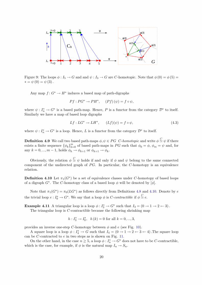
Example 4.11 A triangular loop is a loop φ : I∗3 → G∗ such that I3 = (0→ 1→ 2← 3) .The triangular loop is C-contractible because the following shrinking map
h : I∗3 → I∗0 , h (k) = 0 for all k = 0, ..., 3,
provides an inverse one-step C-homotopy between φ and e (see Fig. 10).A square loop is a loop φ : I∗4 → G such that I4 = (0→ 1→ 2← 3← 4) .The square loop
can be C-contracted to e in two steps as is shown on Fig. 11.On the other hand, in the case n ≥ 5, a loop φ : I∗n → G∗ does not have to be C-contractible,
which is the case, for example, if φ is the natural map In → Sn.
20
G*=0 1 2 3
*=0
*
φ(1)
φ(2)
φ
e
hCh
-
Figure 10: A triangular loop φ is C-contractible.
G
*=0 1 2
*=0
*
φ(1)=ψ(1) φ(2)
ψ
e
h2
Ch-
*=0 1 2 3
φ
4
φ(3)h1
2
Ch-
1
Figure 11: A square loop φ is C-contractible. Note that φ (0) = φ (4) = ψ (0) = ψ (2) = ∗.
4.3 Local description of C-homotopy
We prove here technical results which has a self-sustained meaning for practical work withC-homotopies.
Lemma 4.12 Let a, b be two vertices in a digraph G such that either a = b or a→ b→ a. Thenany path-map φ : In → G, such that φ (i) = a, φ (i + 1) = b, and i→ i+1 in In, is C-homotopicto a path-map φ′ : I ′n → G where I ′n is obtained from In by changing one edge i → i + 1 toi + 1→ i and φ′ (j) = φ (j) for all j = 0, ..., n.
Proof. A C-homotopy between φ and φ′ is constructed in two one-step inverse C-homotopiesas is shown on the following diagram:
φ′ : In′ → G ... ia← i + 1
b...
↓ ↘ ↘ψ : In+1 → G ... i
a→ i + 1
a← i + 2
b...
↑ ↑ ↗φ : In → G ... i
a→ i + 1
b...
The subscript under each element of the line digraph indicates the value of the loop on thiselement.
Any path-map φ : In → G defines a sequence θφ = {vi}ni=0 of vertices of G by vi = φ (i) . By
definition of a path-map, we have for any i = 0, ..., n − 1 one of the following relations:
vi = vi+1, vi → vi+1, vi+1 → vi.
21
If φ is a based path-map, then we have v0 = ∗, if φ is a loop then v0 = ∗ = vn. We consider θφ
as a word over the alphabet VG.
Theorem 4.13 Two loops φ : I∗n → G∗ and ψ : I∗m → G∗ are C-homotopic if and only ifthe word θψ can be obtained from θφ by a finite sequence of the following transformations (orinverses to them):
(i) ...abc... 7→ ...ac... where (a, b, c) is any permutation of a triple (v, v′, v′′) of vertices forminga triangle in G, that is, such that v → v′, v → v′′, v′ → v′′ (and the dots “...” denote theunchanged parts of the words).
(ii) ...abc... 7→ ...adc... where (a, b, c, d) is any cyclic permutation (or a cyclic permutation inthe inverse order) of a quadruple (v, v′, v′′, v′′′) of vertices forming a square in G, that is, suchthat v → v′, v → v′′′, v′ → v′′, v′′′ → v′′.
(iii) ...abcd... 7→ ...ad... where (a, b, c, d) is as in (ii).(iv) ...aba...→ ...a... if a→ b or b→ a.(v) ...aa... 7→ ...a...
Proof. Let us first show that if θφ = θψ then φC' ψ. If, for any edge i→ i+1 (or i← i+1)
in In we have also i→ i + 1 (resp. i← i + 1) in Im then In = Im and φ = ψ (although n = m,the line digraphs In and Im could a priori be different elements of In). Assume that, for somei, we have i → i + 1 in In but i ← i + 1 in Im. Then, by Lemma 4.12, we can change the edgei → i + 1 in In to i ← i + 1 while staying in the same C-homotopy class of φ. Arguing by
induction, we obtain φC' ψ.
We write θφ ∼ θψ if θψ can be obtained from θφ by a finite sequence of transformations
(i) − (v) (or inverses to them). Let us show that θφ ∼ θψ implies that φC' ψ. For that we
construct for each of the transformations (i) − (v) a C-homotopy between φ and ψ. Note thatin this part of the proof φ and ψ can be arbitrary path-maps (not necessarily based).
(i) Assume that a→ c (the case c→ a is similar). Then either b→ c or a→ b (otherwise wewould have got a→ c→ b→ a which is excluded by a triangle hypothesis). The C-homotopiesin the both cases are shown on the diagram:
Im ... a → c ...| � �
In ... a − b → c...
Im ... a → c ...| | �
In ... a → b − c...
Each position here corresponds to a vertex in a cylinder Ch or C−h (that is, in In or Im) and
shows its image (a, b or c) under the map φ resp. ψ. The arrows and undirected segments showsthe edges in the cylinder Ch or C−
h (in particular, horizontal arrows and segments show the edgesin In and Im). The undirected segments, such as a − b and c − b, should be given directionsmatching those on the digraph G.
(ii) Assume as above a → d and b → c. Then we have two-step C-homotopy as on thediagram:
Im ... a → d − c ...↑ ↖ ↖ ↖
In+1 ... a − a → d − c...| | | �
In ... a − b → c ...
22
(iii) Assume a→ d. Then we have b→ c, and the C-homotopy is shown on the diagram:
Im ... ... a → d ...� | | �
In ... a − b → c − d
Note that if a→ b then also d→ c, and if b→ a then also c→ d.(iv) Assuming a→ b we obtain the following C-homotopy:
Im ... ... a ...↙ ↓ ↘
In ... a → b ← a...
(v) Here is the required C-homotopy:
Im ... ... a ...↗ ↑
In ... a − a ...
Before we go to the second half of the proof, observe that the transformation
...abc... 7→ ...ac... (4.4)
of words is possible not only in the case when a, b, c come from a triangle as in (i) but also whena, b, c form a degenerate triangle, that is, when there are identical vertices among a, b, c whiledistinct vertices among a, b, c are connected by an edge. Indeed, in the case a = b we have by(v)
abc = aac ∼ ac,
in the case a = c we have by (iv) and (v)
abc = aba ∼ a ∼ ac,
and in the case b = c by (v)abc = acc ∼ ac.
Now let us prove that φC' ψ implies θφ ∼ θψ. It suffices to assume that there exists an
one-step direct C-homotopy from φ to ψ given by a shrinking map h : I∗n → I∗m. Set
θφ = a0a1...an and θψ = b0b1...bm
where ai, bj ∈ VG and a0 = b0 = an = bm = ∗. For any i = 0, ..., n set j = h (i) and consider twowords
Ai = a0a1...aibj and Bi = b0b1...bj .
We will prove by induction in i that Ai ∼ Bi for all i = 0, ..., n. If this is already known, thenfor i = n we have j = m and
a0a1...anbm ∼ b0b1...bm.
Since anbm = ∗∗ ∼ ∗ = an, it follows that θφ ∼ θψ.Now let us prove that Ai ∼ Bi for all i = 0, ..., n. For i = 0 we have A0 = a0b0 = ∗∗ ∼ ∗ =
b0 = B0. Assuming that Ai ∼ Bi, let us prove that Ai+1 ∼ Bi+1. Let us consider a structure
23
of the cylinder Ch over the edge between i and i + 1 in In. Set h (i) = j, a = ai, a′ = ai+1, b =
bj , b′ = bj+1. There are only the following two cases:
b↗ ↖
a − a′and
b − b′
↑ ↑a − a′
. (4.5)
Note that each arrow on Ch transforms either to an arrow between the vertices of G or to theidentity of the vertices.
Consider first the case of the left diagram in (4.5). In this case b′ = b and we obtain by (4.4)and by the induction hypothesis that
Ai+1 = a0a1...ai−1aa′b ∼ a0a1...ai−1ab = Ai ∼ Bi = Bi+1.
Consider now the case of the right diagram in (4.5) and prove that in this case
which concludes the induction step in this case.In order to prove (4.6) observe first that if all the vertices a, a′, b, b′ are distinct, then they
form a square and (4.6) follows by transformation (ii). In the case a′ = b (4.6) is an equality,and in the case a = b′ the relation (4.6) follows by transformation (iv):
aa′b′ ∼ a = b′ ∼ abb′.
In the case a = b the triple a, a′, b′ is a triangle or a degenerate triangle, and we obtained from(4.4) and (v)
aa′b′ ∼ ab′ ∼ aab′ = abb′,
and the case a′ = b′ is similar. Finally, if a = a′ then similarly by (v) and (4.4) we obtain
aa′b′ = aab′ ∼ ab′ ∼ abb′,
and the case b = b′ is similar.
Remark 4.14 Note that the transformation (iii) was not used in the second half of the proof,so (iii) is logically not necessary in the statement of Theorem 4.13. Note also that (iii) can beobtained as composition of (ii) and (iv) as follows:
abcd ∼ adcd ∼ ad.
However, in applications it is still convenient to be able to use (iii).
Example 4.15 A triangular loop on Fig. 10 is contractible because if a, b, c are vertices of atriangle then
abca ∼ aca ∼ a.
A square loop on Fig. 11 is contractible because if a, b, c, d are vertices of a square then
abcda ∼ ada ∼ a.
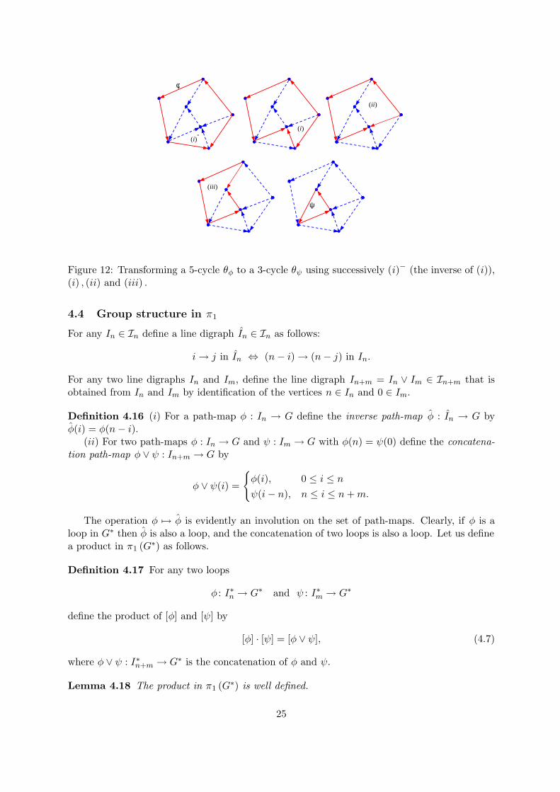
Consider the loops φ and ψ on Fig. 9, that are known to be C-homotopic. It is shown onFig. 12 how to transform θφ to θψ using transformations of Theorem 4.13.
24
(i)-
(i)
(ii )
(iii )
φ
ψ
Figure 12: Transforming a 5-cycle θφ to a 3-cycle θψ using successively (i)− (the inverse of (i)),(i) , (ii) and (iii) .
4.4 Group structure in π1
For any In ∈ In define a line digraph In ∈ In as follows:
i→ j in In ⇔ (n− i)→ (n− j) in In.
For any two line digraphs In and Im, define the line digraph In+m = In ∨ Im ∈ In+m that isobtained from In and Im by identification of the vertices n ∈ In and 0 ∈ Im.
Definition 4.16 (i) For a path-map φ : In → G define the inverse path-map φ : In → G byφ(i) = φ(n− i).
(ii) For two path-maps φ : In → G and ψ : Im → G with φ(n) = ψ(0) define the concatena-tion path-map φ ∨ ψ : In+m → G by
φ ∨ ψ(i) =
{φ(i), 0 ≤ i ≤ n
ψ(i− n), n ≤ i ≤ n + m.
The operation φ 7→ φ is evidently an involution on the set of path-maps. Clearly, if φ is aloop in G∗ then φ is also a loop, and the concatenation of two loops is also a loop. Let us definea product in π1 (G∗) as follows.
Definition 4.17 For any two loops
φ : I∗n → G∗ and ψ : I∗m → G∗
define the product of [φ] and [ψ] by
[φ] ∙ [ψ] = [φ ∨ ψ], (4.7)
where φ ∨ ψ : I∗n+m → G∗ is the concatenation of φ and ψ.
Lemma 4.18 The product in π1 (G∗) is well defined.
25
Proof. Let φ, φ′, ψ, ψ′ be loops of G∗ and let
φC' φ′, ψ
C' ψ′. (4.8)
We must prove that
φ ∨ ψC' φ′ ∨ ψ′. (4.9)
It suffices to consider only the case when the both C-homotopies in (4.8) are one-step C-homotopies. Then we have
φ ∨ ψC' φ′ ∨ ψ
because one-step C-homotopy between φ and φ′ easily extends to that between φ∨ψ and φ′∨ψ.In the same way we obtain
φ′ ∨ ψC' φ′ ∨ ψ′,
whence (4.9) follows.
Lemma 4.19 For any loop φ : I∗n → G∗ we have φ ∨ φC' e where φ is the inverse loop for the
loop φ ande : I∗0 → G∗ (4.10)
is the trivial loop.
Proof. Let θφ = v0...vn. Then θφ = vn...v0 and
θφ∨φ = v0...vn−1vnvn−1...v0.
Using successively the transformations aba 7→ a and aa 7→ a of Theorem 4.13, we obtain that
θφ∨φ ∼ ∗ whence φ ∨ φC' e follows.
Theorem 4.20 Let G,H be digraphs.(i) The set π1(G∗) with the product (4.7) and neutral element [e] from (4.10) is a group. It
will be referred to as the fundamental group of a digraph G∗.(ii) A based digraph map f : G∗ → H∗ induces a group homomorphism
π1(f) : π1(G∗)→ π1(H
∗), (π1(f)) [φ] = [f ◦ φ],
which depends only on homotopy class of f . Hence, we obtain a functor from the category ofdigraphs D∗ to the category of groups.
(iii) Let γ : I∗k → G∗ be a based path-map with γ(k) = v. Then γ induces an isomorphism offundamental groups
γ] : π1(G∗)→ π1(G
v),
which depends only on C-homotopy class of the path-map γ.
Proof. (i) This follows from Lemmas 4.18 and 4.19, since the product in π1(G∗) satisfiesthe associative law, the class [e] ∈ π1(G∗) satisfies the definition of a neutral element, and [φ] isthe inverse of [φ] for any [φ] ∈ π1 (G∗).
(ii) Let φ and ψ be C-homotopic loops in G∗. It follows from Definition 4.5 and (4.2) that
f ◦ φC' f ◦ ψ and, hence, the map π1(f) is well defined.
26
The map π1(f) is a homomorphism because π1([e]) = [e] and, for any two loops φ, φ′ in G∗,
f ◦ (φ ∨ φ′) = (f ◦ φ) ∨(f ◦ φ′) .
If f and g two homotopic based maps from G∗ to H∗ then f ◦φ ' g ◦φ and hence f ◦φC' g ◦φ,
which finishes the proof.(iii) For any loop φ in G∗, define a based loop γ](φ) in Gv by
γ](φ) = γ ∨ φ ∨ γ : Ik+n+k → G,
where γ is the inverse path-map of γ as in Definition 4.16. Similarly to the proof of (ii) andusing Lemma 4.19, one shows that γ] : π1(G, ∗)→ π1(G, v) is a group homomorphism. Since γ]
is obviously the inverse map of γ], it follows that γ] is an isomorphism.If γ1 and γ2 are two C-homotopic path-maps connecting vertices ∗ and v then γ1 ∨ φ ∨ γ1
and γ2 ∨ φ ∨ γ2 are C-homotopic (cf. the proof of Lemma 4.18). Hence, γ] depends only onC-homotopy class of the map γ.
Lemma 4.21 Let f : G∗ → Ha and g : G∗ → Hb be two based digraphs maps. If f ' g :G → H then there exists a based path-map γ : I∗k → Ha with γ (k) = b such that, for any loopφ : I∗n → G∗, we have
γ] (f ◦ φ)C' g ◦ φ. (4.11)
Consequently, the following diagram is commutative:
π1 (G∗)π1(f)−→ π1 (Ha)
↓id ↓γ
]
π1 (G∗)π1(g)−→ π1
(Hb)
Proof. Note that f ◦ φ is a loop in Ha and g ◦ φ is a loop in Hb. It suffices to prove thestatement in the case when f and g are related by an one-step homotopy, that is, f (x)−→=g (x)for all x ∈ VG. In particular, we have a−→=b.
Consider the path-map γ : I → H given by γ (0) = a and γ (1) = b. Then the loop γ] (f ◦ φ) :
I ∨ In ∨ I → Hb is defined by
γ] (f ◦ φ) = γ ∨ (f ◦ φ) ∨ γ.
Define shrinking h : I∨In∨I → In as follows: h on In is identical, and the endpoints of I∨In∨Iare mapped by h to the corresponding endpoints of In:
In 0 ... ... n↑h ↗ ↑ ... ... ↑ ↖
I ∨ In ∨ I −1 ← 0 ... ... n → n + 1
where we enumerate the vertices of I ∨ In ∨ I as {−1, 0, ..., n + 1} .Then we have, for 0 ≤ i ≤ n,
Hence, for all i,γ] (f ◦ φ) (i)−→= (g ◦ ϕ) (h (i)) ,
which implies (4.11) by (4.2).
Theorem 4.22 Let G,H be two connected digraphs. If G ' H then the fundamental groupsπ1 (G∗) and π1 (H∗) are isomorphic (for any choice of the based vertices).
Proof. Let f : G → H and g : H → G be homotopy inverses maps (cf. 3.4). ApplyingLemma 4.21 to f ◦ g ' idG and to g ◦ f ' idH , we obtain the result by a standard argument (cf.[12, Ch.1, Thm 8]).
4.5 Relation between H1 and π1
One of our main results is the following theorem.
Theorem 4.23 For any based connected digraph G∗ we have an isomorphism
π1(G∗) /[π1(G
∗), π1(G∗)] ∼= H1(G,Z)
where [π1(G∗), π1(G∗)] is a commutator subgroup.
Proof. The proof is similar to that in the classical algebraic topology [8, p.166]. For anybased loop φ : I∗n → G∗ of a digraph G∗, define a 1-path χ(φ) on G as follows: χ(φ) = 0 forn = 0, 1, 2, and for n ≥ 3
χ (φ) =∑
{i:i→i+1}
eφ(i)φ(i+1) −∑
{i:i+1→i}
eφ(i+1)φ(i), (4.12)
where the summation index i runs from 0 to n − 1. It is easy to see that the 1-path χ (φ) isallowed and closed and, hence, determines a homology class [χ (φ)] ∈ H1 (G,Z). Let us firstprove that, for any two based loops φ : I∗n → G∗ and ψ : I∗m → G∗,
φC' ψ ⇒ [χ(φ)] = [χ(ψ)] . (4.13)
Note that any based loop with n ≤ 2 is C-homotopic to trivial. For n ≥ 3, it is sufficiently to
check (4.13) assuming that φC' ψ is given by an one-step direct C-homotopy with a shrinking
map h : I∗n → I∗m. Setφ′ := ψ ◦ h : I∗n → G∗
and observe that by (4.12) χ(φ′) = χ (ψ) . It remains to show that [χ (φ)] =
[χ(φ′)] .
By Remark 4.6 the digraph maps φ and φ′, acting from In to G, are homotopic. Denote bySn the digraph that is obtained from In by identification of the vertices 0 and n (that is, Sn isa cycle digraph from Example 2.8). Then ϕ and φ′ can be regarded as digraph maps from Sn
to G, and they are again homotopic as such.Consider the standard homology class [$] ∈ H1 (Sn) given by (2.8). Comparing (2.8) and
(4.12), we see thatφ∗ ($) = χ (ϕ) and φ′
∗ ($) = χ(φ′) .
28
On the other hand, by Theorem 3.3 we have [φ∗ ($)] =[φ′∗ ($)
], which finishes the proof of
(4.13).Hence, χ determines a map
χ∗ : π1(G∗)→ H1(G,Z), χ∗[φ] = [χ(φ)].
The map χ∗ is a group homomorphism because, for based loops φ, ψ and the neutral element[e] ∈ π1 (G∗), we have χ∗([e]) = 0 and
Since the group H1(G,Z) is abelian, it follows that
[π1(G∗), π1(G
∗)] ⊂ Ker χ∗.
Now let us prove that χ∗ is an epimorphism. Define a standard loop on G as a finite sequencev = {vk}
nk=0 of vertices of G such that v0 = vn and, for any k = 0, ..., n− 1, either vk → vk+1 or
vk+1 → vk. For a standard loop v define an 1-path
$v =∑
{k:vk→vk+1}
evkvk+1−
∑
{k:vk+1→vk}
evkvk+1(4.14)
and observe that $v is allowed and closed. The 1-paths of the form (4.14) will be referred to asstandard paths. Consider an arbitrary closed 1-path
w =∑
k
nkeikjk∈ Ω1(G,Z).
Since ∂w = 0 and ∂eij = ej − ei, the path w can be represented as a finite sum of standardpaths. Hence, in order to prove that χ∗ is an epimorphism, it suffices to show that any standard1-path $v is in the image of χ. Note that the standard loop v determines naturally a basedloop φ : I∗n → Gv0 by φ (i) = vi. Since the digraph G is connected, there exists a based pathf : I∗s → G∗ with f(s) = v0. Thus we obtain a based loop
f ∨ φ ∨ f : I∗2s+n → G∗.
It follows directly from our construction, that χ(f∨φ∨f) = $v, and hence χ∗ is an epimorphism.We are left to prove that
Ker χ∗ ⊂ [π1(G∗), π1(G
∗)].
For that we need to prove that, for any loop φ : I∗n → G∗, if χ∗([φ]) = 0 ∈ H1(G,Z), then [φ]lies in the commutator [π1(G∗), π1(G∗)]. In the case n ≤ 2 any loop φ is C-homotopic to thetrivial loop. Assuming in the sequel n ≥ 3, we use the word θφ = v0v1...vn where vi = φ (i).
Consider first the case, when χ(φ) = 0 ∈ Ω1(G). Since the digraph G is connected, for anyvertex vi there exists a based path-map ψi : I∗pi
→ G∗ with ψi(pi) = vi. If vi = vj for some i, jthen we make sure to choose ψi and ψj identical. For i = 0 and i = n choose ψi to be trivialpath-map e : I∗0 → G∗. For any i = 0, ..., n − 1 define path-map φi : I± → G by the conditionsφi(0) = vi, φi(1) = vi+1 and consider the following loop
(see Fig. 13).Using transformation (iv) of Theorem 4.13 (similarly to the proof of Lemma 4.19), we obtain
thatγ
C' φ0 ∨ φ1 ∨ ... ∨ φn−1 = φ.
On the other hand, it follows from (4.15) that
[γ] =n−1∏
i=0
[ψi ∨ φi ∨ ψi+1
]
Consider for some i = 0, ..., n− 1, such that i→ i + 1, the vertices a = vi and b = vi+1. If a = bthen the loop ψi ∨ φi ∨ ψi+1 is C-homotopic to e. Assume a 6= b, so that a→ b. Then the termeab is present in the right hand side of the identity (4.12) defining χ (φ). Due to χ (φ) = 0, theterm eab should cancel out with −eab in the right hand side of (4.12). Therefore, there existsj = 0, ..., n − 1 such that j + 1→ j, vj+1 = a and vj = b. It follows that
ψj ∨ φj ∨ ψj+1 = ψi+1 ∨ φi ∨ ψi,
and that the loops [ψi ∨ φi ∨ ψi+1
]and
[ψj ∨ φj ∨ ψj+1
](4.16)
are mutually inverse. Therefore, [γ] is a product of pairs of mutually inverse loops, which impliesthat [γ] = [φ] lies in the commutator of π1.
Now consider the general case, when χ (φ) ∈ Ω1 (G) is exact, that is, χ(φ) = ∂ω for some ω ∈Ω2(G). Recall that by Proposition 2.9 any 2-path ω ∈ Ω2 can be represented in the form
ω =N∑
j=1
κjσj
where N ∈ N, κl = ±1 and σl is one of the following 2-paths: a double edge, a triangle, a square.Further proof goes by induction in N . In the case N = 0 we have ω = 0 which was alreadyconsidered above.
In the case N ≥ 1 choose an arbitrary index i = 0, ..., n − 1 such that the vertices a = φ (i)and b = φ (i + 1) are distinct. Assume for certainty that i→ i + 1 and, hence, a → b (the case
30
*
a b
σl φ
c
φ '
Figure 14: Loops φ and φ′ in the case when σl is a triangle.
i + 1→ i can be handled similarly). Then eab enters χ (φ) with the coefficient 1. Since
χ (φ) = ∂ω =N∑
j=1
κj∂σj ,
there exists σl such that ∂σl contains a term κleab. Fix this l and define a new loop φ′ as follows.If σl is a double edge a, b, a, then consider a loop φ′ that is obtained from φ : I∗n → G∗ by
changing one edge i→ i + 1 in In to i→ i + 1. Then by Lemma 4.12 we have φ′ C' φ.
Let σl be a triangle with the vertices a, b, c. Noticing that
θφ = ...ab...
consider a loop φ′ such thatθφ′ = ...acb...
(see Fig. 14).If σl is a square with the vertices a, b, c, d, then we define a loop φ′ so that
θφ′ = ...adcb.
By Theorem 4.13, we have in the both cases φ′ C' φ and, hence,
[φ′] = [φ].
By construction, χ(φ′) contains no longer the term eab. On the other hand, we will prove
below that, for some κ = ±1,χ(φ′) = χ (φ)− κ∂σl. (4.17)
Comparing the coefficients in front of eab in the both parts of (4.17), we obtain the identity0 = 1− κκl whence κ = κl. It follows from (4.17) with κ = κl that
χ(φ′) = χ (φ)− ∂ (κlσl) = ∂ω − ∂ (κlσl) = ∂ω′,
whereω′ =
∑
j 6=l
cjσj .
By the inductive hypothesis we conclude that[φ′] lies in the commutator [π1(G∗), π1(G∗)],
whence the same for [φ] follows.
31
We are left to prove the identity (4.17). If σl is a double edge a, b, a then
χ(φ′)− χ (φ) = −eba − eab = −∂eaba = −∂σl.
If σl is a trianglec
� �a −→ b
then we obtain a cycle digraph S3 with the vertices a, b, c, and if σl is a square
d −→ c| |a −→ b
then we obtain a cycle digraph S4 with the vertices a, b, c, d. Let $ be the standard 1-path onS3 in the first case and that on S4 in the second case (see (2.8)). Then it is easy to see that
χ (φ)− χ(φ′) = $,
and (4.17) follows from the observation that ∂σl = ±$ (cf. Example 2.8).
4.6 Higher homotopy groups
Recall that, for any based digraph G∗, a based loop-digraph LG∗ was defined in Definition 4.8,and, for a digraph map f : G∗ → H∗, we defined a digraph map Lf : LG∗ → LH∗ by (4.3).
Definition 4.24 For any digraph G∗ let LnG = LnG∗, n = 0, 1, 2, 3, . . . be based digraphsdefined inductively as
L0G∗ = G∗, L1G∗ = LG∗, and, for n ≥ 2, LnG∗ def= L
(Ln−1G∗)
where the base point in LG∗ is the based map I∗0 → G∗ which we also denote by ∗.For n ≥ 2, define homotopy group πn(G∗) of the digraph G∗ inductively by
πn(G∗) = πn−1(LG∗).
Theorem 4.25 Let G∗, H∗ be two based digraphs. If f and g are homotopic digraph mapsG∗ → H∗ then Lf and Lg are homotopic digraph maps LG∗ → LH∗. If G∗ ' H∗ then alsoLG∗ ' LH∗.
Proof. In the first statement, it suffices to consider the case of one-step homotopy betweenf and g, which by (3.2) amounts to either f (x)−→=g (x) for all x ∈ VG or g (x)−→=f (x) for allx ∈ VG. Assume without loss of generality that
f (x)−→=g (x) for all x ∈ VG.
Then, for any loop ψ ∈ LG∗, ψ : I∗n → G∗, we have also
f (ψ (i))−→=g (ψ (i)) for all i = 0, ..., n,
which implies that f ◦ ψ and g ◦ ψ are one-step homotopic and, hence, one-step C-homotopic.Therefore, the loops f ◦ ψ and g ◦ ψ as elements of LH∗ are either identical or connected by anedge in LH∗, that is
(Lf) (ψ)−→= (Lg) (ψ) for all ψ ∈ VLG.
Hence, Lf ' Lg, which finishes the proof of the first statement.Since L is a functor we obtain the proof of the rest part of the Theorem.
32
2
1
1
1
1
2
2
2 3
3
3
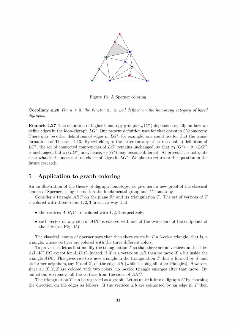
Figure 15: A Sperner coloring
Corollary 4.26 For n ≥ 0, the functor πn is well defined on the homotopy category of baseddigraphs.
Remark 4.27 The definition of higher homotopy groups πn (G∗) depends crucially on how wedefine edges in the loop-digraph LG∗. Our present definition uses for that one-step C-homotopy.There may be other definitions of edges in LG∗, for example, one could use for that the trans-formations of Theorem 4.13. By switching to the latter (or any other reasonable) definition ofLG∗, the set of connected components of LG∗ remains unchanged, so that π1 (G∗) = π0 (LG∗)is unchanged, but π1 (LG∗) and, hence, π2 (G∗) may become different. At present it is not quiteclear what is the most natural choice of edges in LG∗. We plan to return to this question in thefuture research.
5 Application to graph coloring
An an illustration of the theory of digraph homotopy, we give here a new proof of the classicallemma of Sperner, using the notion the fundamental group and C-homotopy.
Consider a triangle ABC on the plane R2 and its triangulation T . The set of vertices of Tis colored with three colors 1, 2, 3 in such a way that
• the vertices A,B,C are colored with 1, 2, 3 respectively;
• each vertex on any side of ABC is colored with one of the two colors of the endpoints ofthe side (see Fig. 15).
The classical lemma of Sperner says that then there exists in T a 3-color triangle, that is, atriangle, whose vertices are colored with the three different colors.
To prove this, let us first modify the triangulation T so that there are no vertices on the sidesAB,AC,BC except for A,B,C. Indeed, if X is a vertex on AB then we move X a bit inside thetriangle ABC. This gives rise to a new triangle in the triangulation T that is formed by X andits former neighbors, say Y and Z, on the edge AB (while keeping all other triangles). However,since all X,Y, Z are colored with two colors, no 3-color triangle emerges after that move. Byinduction, we remove all the vertices from the sides of ABC.
The triangulation T can be regarded as a graph. Let us make it into a digraph G by choosingthe direction on the edges as follows. If the vertices a, b are connected by an edge in T then
33
choose direction between a, b using the colors of a, b and the following rule:
1→ 2, 2→ 3, 3→ 11� 1, 2� 2, 3� 3
(5.1)
Assume now that there is no 3-color triangle in T. Then each triangle from T looks in G like
•↗ ↖
• � •or
•↙ ↘
• � •or
•↗↙ ↘↖
• � •,
in particular, each of them contains a triangle in the sense of Theorem 4.13. Using the trans-formations (ii) and (iv) of Theorem 4.13 and the partition of G into the triangles, we contractany loop on G to an empty word (cf. Fig. 14), whence π1 (G∗) = {0}.
Consider now a colored cycle S3
1↗ ↘
3 ←− 2(5.2)
and the following two maps: f : G→ S3 that preserves the colors of the vertices and g : S3 → Gthat maps the vertices 1, 2, 3 of S3 onto A,B,C, respectively. Both f, g are digraph maps, whichfor the case of f follows from the choice (5.1) of directions of the edges of G. Since f ◦ g = idS3 ,we obtain that π1 (f ◦ g) = π1 (f) ◦ π1 (g) is an isomorphism of π1 (S3) ' Z onto itself, which isnot possible by π1 (G∗) = {0} .
6 Homology and homotopy of (undirected) graphs
A homotopy theory of undirected graphs was constructed in [1] and [2] (see also [4]). Here weshow that this theory can be obtained from our homotopy theory of digraphs as restriction toa full subcategory. The same restriction enables us to define a homotopy invariant homologytheory of undirected graphs such that the classical relation between fundamental group andthe first homology group given by Theorem 4.23 is preserved. In particular, the so obtainedhomology theory for graphs answers a question raised in [1, p.32].
To distinguish digraphs (see Definition 2.1) and (undirected) graphs (see Definition 3.1 below)we use the following notations. To denote a digraph and its sets of vertices and edges, we useas in the previous sections the standard font as G = (VG, EG). To denote a graph and its setsof vertices and edges, we will use a bold font, for example, G = (VG,EG). The bold font willalso be used to denoted the maps between graphs.
Definition 6.1 (i) A graph G = (VG,EG) is a couple of a set VG of vertices and a subsetEG ⊂ {VG × VG \ diag} of non-ordered pairs of vertices that are called edges. Any edge(v, w) ∈ EG will be also denoted by v ∼ w.
(ii) A morphism from a graph G = (VG,EG) to a graph H = (VH,EH) is a map
f : VG → VH
such that for any edge v ∼ w on G we have either f (v) = f (w) or f (v) ∼ f (w). We will referto morphisms of graphs as graph maps.
34
To each graph G = (VG,EG) we associate a digraph G = (VG, EG) where VG = VG andEG is defined by the condition v → w ⇔ v ∼ w. Clearly, the digraph G satisfies the conditionw → v ⇔ v → w. Any digraph with this property will be called a double digraph.
The set of all graphs with graph maps forms a category (which was also introduced by [1]and [2]), that will be denoted by G.
The assignment G 7→ G and a similar assignment f 7→ f of maps, that is well defined,provide a functor O from G to D. It is clear that the image O is a full subcategory O(G) of Dthat consists of double digraphs, such that the inverse functor O−1 : O(G)→ G is well defined.
Definition 6.2 For two graphs G = (VG,EG) and H = (VH,EH) define the Cartesian productG �H as a graph with the set of vertices VG ×VH and with the set of edges as follows: forx, x′ ∈ VG and y, y′ ∈ VH, we have (x, y) ∼ (x′, y′) in G�H if and only if
either x′ = x and y ∼ y′, or x ∼ x′ and y = y′.
The comparison of Definitions 2.3 and 6.2 yields the following statement.
Lemma 6.3 The functors O and O−1 preserve the product �, that is
O(G�H) = G�H, O−1(G�H) = G�H.
By definition, a line graph is a graph Jn = (V,E) with V = {0, 1, . . . , n} and E = {k ∼k + 1|0 ≤ k ≤ n− 1}. Let J = {0 ∼ 1} be the line graph with two vertices. Let Jn = O(Jn) andJ = O(J).
Definition 6.4 [2] Let G,H be two graphs.(i) Two graph maps f ,g : G→ H are called homotopic if there exists a line graph Jn (n ≥ 0)
and a graph map F : G� Jn → H such that
F|G�{0} = f0 and F|G�{n} = f1
In this case we shall write f ' g.(ii) The graphs G and H are called homotopy equivalent if there exist graph maps f : G→ H
and g : H→ G such thatf ◦ g ' idH, g ◦ f ' idG . (6.1)
In this case we shall write H ' G. The maps f and g are as in (6.1) called homotopy inversesof each other.
The relation ”'” is an equivalence relation on the set of graph maps and on the set of graphs(see [2]).
Proposition 6.5 Let f ,g : G → H be graph maps. The maps f and g are homotopic if andonly if the digraph maps f = O(f) and g = O(g) are homotopic.
Proof. Let F : G � Jn → H be a homotopy between f and g as in Definition 6.4. Thenatural digraph inclusion In → Jn (where In ∈ I is arbitrary) induces the digraph inclusionΘ: G � In → G � Jn. Applying functor O and Lemma 6.3 we obtain a digraph map F : =G� Jn → H such that the composition F ◦Θ: G� In → H provides a digraph homotopy. Nowlet F : G � In → H be a digraph homotopy as in Definition 3.1 between two double digraphs.Define a digraph map F ′ : G � Jn → H on the set of vertices by F ′(x, i) = F (x, i). Since H is
35
a double digraph, this definition is correct. Applying functor O−1 and Lemma 6.3 we obtain agraph homotopy F′ : G� Jn → H.
Denote by D′ the homotopy category of digraphs. The objects of this category are digraphs,and the maps are classes of homotopic digraphs maps. Similarly, denote by G′ the homotopycategory of graphs and by O(G′) the homotopy category of double digraphs.
Proposition 6.5 implies the following.
Corollary 6.6 The functors O and O−1 induce an equivalence between homotopy category ofgraphs and homotopy category of double digraphs
Definition 6.7 Let K be a commutative ring with unity. Define homology groups of a graph Gwith coefficients in K as follows: Hn(G,K) : = Hn(G,K) where G = O (G) .
The following statement follows from Theorem 3.3 and Proposition 6.5.
Proposition 6.8 The homology groups of a graph G with coefficients K are homotopy invariant.
A (induced) subgraph H of a graph G is a graph whose set of vertices is a subset of that ofG and the edges of H are all those edges of G whose adjacent vertices belong to H.
Definition 6.9 Let G be a graph and H be its subgraph.(i) A retraction of G onto H is a graph map r : G→ H such that r|H = idH .(ii) A retraction r : G→ H is called a deformation retraction if i◦r ' idG, where i : H→ G
is the natural inclusion map.
Note that the condition i ◦ r ' idG is equivalent to the existence of a graph morphismF : G� Jn → G such that
F|G�{0} = idG, F|G�{n} = i ◦ r. (6.2)
Similarly Proposition 3.5, a deformation retraction provides homotopy equivalence G ' H withhomotopy inverse maps i, r (compare with [2, p.119]).
Example 6.10 (i) Let us define a cycle graph Sn (n ≥ 3) as the graph that is obtained fromJn by identifying of the vertices n and 0. Then
Hp(Sn,K) =
K, ∀n and p = 0,
K, n ≥ 5 and p = 1,
0, in other cases.
(ii) Let G be a star-like graph, that there is a vertex a ∈ VG such that a ∼ v for anyv ∈ VG. Then the map r : G → {a} is a deformation retraction which implies G ' {a} (cf.Example 3.11). Consequently, H0(G,K) = K and Hp(G,K) = 0 for all p > 0.
(iii) If a graph G is a tree, then G is contractible (cf. Example 3.10). In particular,H0(G,K) = K and Hp(G,K) = 0 for all p > 0.
Definition 6.11 Let f : G→ H be a graph map. The cylinder Cf of f is a graph with the setof vertices VCf
= VG tVH and with the set of edges ECfthat consists of all the edges from
EG and EH as well as of the edges of the form x ∼ f (x) for all x ∈ VG.
36
Analogously to Proposition 3.18, we obtain the following.
Proposition 6.12 We have a homotopy equivalence Cf ' H.
Below we consider based graphs G∗, where ∗ is a based vertex of G. The based vertex of Jn
will be usually 0.
Definition 6.13 Let G be a graph. A path-map in a graph G is any graph map Φ : Jn → G.A based path on based graph G∗ is a based map Φ : J∗
n → G∗. A loop in G is a based path-mapΦ : J∗
n → G∗ such that Φ(n) = ∗.
The inverse path-map and the concatenation of path-maps are defined similarly to Defini-tion 4.16.
Definition 6.14 (i) A graph map h : Jn → Jm is called shrinking if h (0) = 0, h(n) = m, andh (i) ≤ h (j) whenever i ≤ j.
An extension of a based path-map Φ : J∗m → G∗ is any path-map ΦE = Φ ◦ h where
h : J∗n → J∗
m is shrinking. An extension ΦE is called a stabilization of Φ if the shrinking map hsatisfies the condition h|Jm = id. A stabilization of Φ will be denoted by ΦS .
(ii) Two loops Φ, Ψ in a based graph G∗ are called S-homotopic if there exist stabilizations
ΦS , ΨS which are homotopic. In this case we shall write ΦS' Ψ. This is an equivalence relation
and equivalence class of a loop Φ will be denoted by [Φ] (cf. [1] and [2]).
Define a set π1(G∗) as the set of S-equivalence classes of loops in G∗, and the product inπ1(G∗) by [Φ] ∙ [Ψ] : = [Φ ∨Ψ]. Let e : J∗
0 → G∗ be the trivial loop.
Proposition 6.15 [1], [2, Proposition 5.6] The set π1(G∗) with the product defined above andwith the neutral element [e] is a group, that will be referred to as a fundamental group of thegraph G∗ and denoted by π1 (G∗).
Definition 6.16 Consider two based path-maps
Φ: J∗n → G∗ and Ψ: J∗
m → G∗.
An one-step C-homotopy from Φ to Ψ is given by a shrinking map h : Jn → Jm such that themap F : VCh
→ VG given by
F|Jn = Φ and F|Jm = Ψ,
is a graph map from Ch to G.The path-maps Φ and Ψ are said to be C-homotopic if there exists a sequence of one-step
C-homotopies that connect Φ and Ψ. We shall write in this case ΦC' Ψ.
The following statement follows immediately from definitions of the functor O and cylinderof the graph and digraph maps.
Lemma 6.17 Let h : G → H be a graph map. There exists a natural digraph inclusion Ch →O(Ch), where Ch is a cylinder of the digraph map h : G→ H.
Theorem 6.18 Let G∗ be a based double digraph. We have a natural isomorphism of funda-mental groups π1(G∗) ∼= π1(G∗) where G∗ = O−1(G∗).
37
Proof. Let Φ: J∗n → G∗ be a based loop. Denote by Is
n the special line digraph withthe vertices 0, 1, ..., n and edges i → i + 1 for all i = 0, ..., n − 1. There is a natural inclusionτ : Is
n → Jn. The composition O(Φ) ◦ τ : Isn∗ → G∗ defines a based loop φ in G∗. At first we
would like to prove, that the correspondence Φ −→ O(Φ) ◦ τ = φ provides a well defined mapof sets
O∗ : π1(G∗)→ π1(G
∗), O∗([Φ]) 7→ [O(Φ) ◦ τ ] = [φ].
Let Φ: J∗k → G∗, Ψ: J∗
m → G∗ be loops and ΦS' Ψ. The homotopic stabilizations ΦS and ΨS
provide one-step C-homotopies ΦS C' Φ, ΨS C
' Ψ. A homotopy between ΦS and ΨS provides
C-homotopy ΦS C' ΨS . Since C-homotopy is an equivalence relation, we obtain Φ
C' Ψ. Now by
Lemma 6.17 we obtain that φC' ψ. That is the map O∗ is well defined, and it is easy to see that
this is a homomorphism of groups. This is an epimorphism as follows from Proposition 4.12.Digraph maps
φ : Isn∗ → G∗, ψ : Is
m∗ → G∗
define graphs mapsΦ: Jn → G∗, Φ: Jm → G∗,
such that O(Φ) ◦ τ = φ and O(Ψ) ◦ τ = ψ. A one-step C-homotopy φC' ψ implies a one-step
C-homotopy ΦC' Ψ. That implies that ΦE is homotopic to Ψ or vice versa. To finish the proof
of the Theorem, it suffices to prove that ΦS' Ψ. But this follows directly from definition of
fundamental group of graph in [1] and [2].
Theorem 6.19 For any based graph G∗ we have an isomorphism
π1(G∗)/[π1(G
∗), π1(G∗)] ∼= H1(G,Z)
where [π1(G∗), π1(G∗)] is a commutator subgroup.
Proof. Follows from Theorems 6.18 and 4.23.
Definition 6.20 [1, p.41] Let G∗ be a based graph.(i) A based path graph PG∗ is a graph with the set of vertices VPG∗ = {Φ: Jn → G∗}, a
base vertex ∗ : J0 → G∗, and there is an edge Φ ∼ Ψ if and only ΦS ' Ψ or Φ ' ΨS .(ii) A based loop graph LG∗ is a based sub-graph of PG∗ with the set of vertices VLG∗ =
{Φ: Jn → G∗|Φ(n) = ∗} and with the restricted from PG∗ set of vertices.(iii) Define higher homotopy groups πn(G∗) : = πn−1(LG∗) for n ≥ 2.
Proposition 6.21 Let G∗ = O(G∗) be a based double digraph. Then LG∗ be a double digraph
and we have a natural inclusion l : LG∗ ⊂→ O−1(LG∗) that is an identity map on the set of
vertices. This map induces a homomorphism of homotopy groups πn(LG∗) → πn(LG∗) forn ≥ 1 and an isomorphism for n = 0.
Proof. The proof that LG∗ is a double digraph is similar to the proof of Proposition 6.5and the graph map l is well defined by Lemma 6.17. Then the result follows.
38
References
[1] Eric Babson, Helene Barcelo, Mark de Longueville, and Reinhard Laubenbacher, Homotopytheory of graphs, Journal Algebr. Comb. 24 (2006), 31–44.
[2] Helene Barcelo, Xenia Kramer, Reinhard Laubenbacher, and Christopher Weaver, Founda-tions of a connectivity theory for simplicial complexes, Advances in Appl. Mathematics 26(2001), 97–128.
[3] Marshall M. Cohen, A course in simple-homotopy theory, Berlin, New York: Springer-Verlag, 1973.
[4] Anton Dochtermann, Homotopy groups of Hom complexes of graphs, Journal of Combina-torial Theory, Series A 116 (2009), 18–194.
[5] Alexander Grigor’yan, Yong Lin, Yuri Muranov, and Shing-Tung Yau, Homologies of pathcomplexes and digraphs, Math arXiv: 1207.2834v4 (2013).
[6] , Cohomology of digraphs and (undirected) graphs, to appear in Asian Journal ofMathematics (2014).
[7] Alexander Grigor’yan, Yuri Muranov, and Shing-Tung Yau, Graphs associated with simpli-cial complexes, Homology, Homotopy, and Applications 16 (2014), 295–311.
[8] Allen Hatcher, Algebraic Topology, Cambridge University Press, 2002.
[9] Alexander V. Ivashchenko, Contractible transformations do not change the homology groupsof graphs, Discrete Math. 126 (1994), 159–170.
[10] S. MacLane, Homology, Die Grundlehren der mathematischen Wissenschaften. Bd. 114.Berlin-Gottingen-Heidelberg: Springer-Verlag, 522 pp. , 1963.
[11] P. Ribenboim, Algebraic structures on graphs, Algebra Universalis 16 (1983), 105–123.