Choosing the Right Algorithm & GuidingPHIL IPP SLUSALLEK & PASCAL GRITTMANN

Topics for TodayWhat does an implementation of a high-performance renderer look like?

Review of algorithms – which to choose for production rendering?

Path guiding – how path tracers can handle complex illumination

Brief look at our current research goal: How to adapt VCM to input scenes?

Choosing the Right Rendering AlgorithmREVIEW AND COMPARISON OF THE ALGORITHMS DISCUSSED SO FAR

Path Tracing – Kajiya 1986Straightforward Monte Carlo integration of the Rendering Equation

Shoot rays from the eye into the scene

Sample incoming direction at hit points

Shoot secondary ray

Optimization: next event estimation

𝐿𝑜 𝑥, 𝜔0 = 𝐿𝑒 𝑥, 𝜔0 + 𝐻(𝑥)𝐿𝑖 𝑥, 𝜔𝑖 𝑓𝑟( 𝜔𝑖 , 𝑥, 𝜔𝑜) 𝑐𝑜𝑠𝜃𝑖 𝑑𝜔𝑖

“Light Transport Equation”

Path Tracing – properties+ Simple to implement

+ Efficient at direct illumination

− Inefficient at caustics

− Inefficient at indirect illumination

Path Tracing – difficult cases

Light Tracing – Dutré et al 1993Reverse of Path Tracing

Path Tracing: Shoot importance into the scene, gather radiance

Light Tracing: Shoot particles into the scene, gather importance

Next Event Estimation: Only way to get contribution for camera with no actual surface

𝑊𝑜 𝑥, 𝜔0 = 𝑊𝑒 𝑥, 𝜔0 + 𝐻(𝑥)𝑊𝑖 𝑥, 𝜔𝑖 𝑓𝑟( 𝜔𝑖 , 𝑥, 𝜔𝑜) 𝑐𝑜𝑠𝜃𝑖 𝑑𝜔𝑖

“Importance Transport Equation”

Light Tracing is efficient at rendering indirect illuminationPATH TRACING LIGHT TRACING

Light Tracing is efficient at rendering causticsPATH TRACING LIGHT TRACING

Light Tracing – properties+ (reasonably) good at indirect illumination

+ efficient at rendering directly visible caustics

- In non-trivial scenes: Wastes A LOT of samples in regions of the scene that do not contribute at all! (The solutions to this are either Metropolis or Guiding).

10

Bidirectional Path Tracing (BPT): Veach & Guibas ´94, Lafortune & Willems ´93 Combines Light Tracing and Path Tracing

Connect eye and light paths

Combine contributions with MIS:

1. Direct Illumination

2. Randomly hitting light

3. Connecting to the eye

4. Connecting eye and light paths

11

Multiple Importance Sampling (MIS) –Veach and Guibas 1995Combine samples from different techniques

Use weighting to select sample with lower variance

σ𝑖=1𝑛 1

𝑛𝑖σ

𝑗=1𝑛𝑖 𝑤𝑖 𝑋𝑖,𝑗

𝑓 𝑋𝑖,𝑗

𝑝𝑖(𝑋𝑖,𝑗)

Power heuristic:

𝑤𝑖 =𝑛𝑖𝑝𝑖

𝛽

σ𝑘 𝑛𝑘𝑝𝑘𝛽 =

1

1+σ𝑘≠𝑖𝑛𝑘𝑝𝑘

𝛽

𝑛𝑖𝑝𝑖𝛽

Balance heuristic:

𝑤𝑖 =1

1+σ𝑘≠𝑖𝑛𝑘𝑝𝑘𝑛𝑖𝑝𝑖

12

𝑓(𝑥)

𝑝1(𝑥)

𝑝2(𝑥)

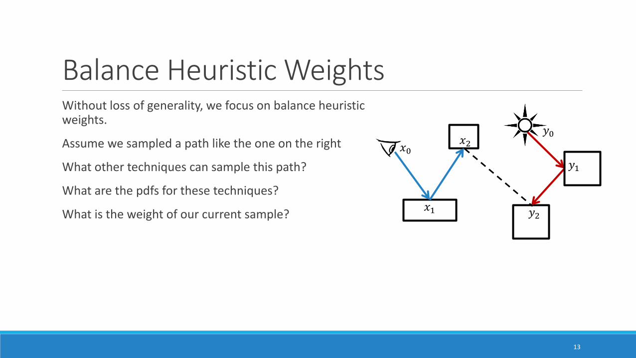
Balance Heuristic WeightsWithout loss of generality, we focus on balance heuristic weights.

Assume we sampled a path like the one on the right

What other techniques can sample this path?

What are the pdfs for these techniques?

What is the weight of our current sample?

13

𝑥0

𝑥1

𝑥2

𝑦0

𝑦1

𝑦2

Techniques on the light sub-path

14

𝑥0

𝑥1

𝑥2 𝑦0

𝑦1

𝑦2

𝑥0

𝑥1

𝑥2 𝑦0

𝑦1

𝑦2

𝑥0

𝑥1

𝑥2 𝑦0

𝑦1

𝑦2

𝑥0

𝑥1

𝑥2 𝑦0

𝑦1

𝑦2

current technique (actually sampled)

Light sub-path PDFs – current techniqueFor simplicity, and without loss of generality, we ignore the number of samples from each technique

The PDF of the current technique is the product of:

𝑝𝑐𝑎𝑚 𝑥0 → 𝑥1 𝑝𝑏𝑟𝑑𝑓 𝑥0 → 𝑥1 → 𝑥2

𝑝𝑙𝑖𝑔ℎ𝑡 𝑦0 → 𝑦1 𝑝𝑏𝑟𝑑𝑓(𝑦0 → 𝑦1 → 𝑦2)

𝑝𝑐𝑜𝑛𝑛 𝑥2, 𝑦2

15

𝑥0

𝑥1

𝑥2 𝑦0

𝑦1

𝑦2

Light sub-path PDFs – connection instead of the last bounce𝑝𝑐𝑎𝑚 𝑥0 → 𝑥1 𝑝𝑏𝑟𝑑𝑓 𝑥0 → 𝑥1 → 𝑥2 𝑝𝑏𝑟𝑑𝑓(𝑥1 → 𝑥2 → 𝑦2)

𝑝𝑙𝑖𝑔ℎ𝑡 𝑦0 → 𝑦1

𝑝𝑐𝑜𝑛𝑛 𝑦2, 𝑦1

16

𝑥0

𝑥1

𝑥2 𝑦0

𝑦1

𝑦2

Light sub-path PDFs – Next Event Estimation𝑝𝑐𝑎𝑚 𝑥0 → 𝑥1 𝑝𝑏𝑟𝑑𝑓 𝑥0 → 𝑥1 → 𝑥2 𝑝𝑏𝑟𝑑𝑓 𝑥1 → 𝑥2 → 𝑦2 𝑝𝑏𝑟𝑑𝑓(𝑥2 → 𝑦2 → 𝑦1)

𝑝𝑐𝑜𝑛𝑛 𝑦0, 𝑦1

17

𝑥0

𝑥1

𝑥2 𝑦0

𝑦1

𝑦2

Light sub-path PDFs – Unidirectional Path Tracing𝑝𝑐𝑎𝑚 𝑥0 → 𝑥1 𝑝𝑏𝑟𝑑𝑓 𝑥0 → 𝑥1 → 𝑥2 𝑝𝑏𝑟𝑑𝑓 𝑥1 → 𝑥2 → 𝑦2 𝑝𝑏𝑟𝑑𝑓 𝑥2 → 𝑦2 → 𝑦1 𝑝𝑏𝑟𝑑𝑓 𝑦2 → 𝑦1 → 𝑦0

18

𝑥0

𝑥1

𝑥2 𝑦0

𝑦1

𝑦2

Combined MIS Denominator1

+𝑝𝑐𝑎𝑚 𝑥0→𝑥1 𝑝𝑏𝑟𝑑𝑓 𝑥0→𝑥1→𝑥2 𝑝𝑏𝑟𝑑𝑓 𝑥1→𝑥2→𝑦2 𝑝𝑙𝑖𝑔ℎ𝑡 𝑦0→𝑦1 𝑝𝑐𝑜𝑛𝑛 𝑦2,𝑦1

𝑝𝑐𝑎𝑚 𝑥0→𝑥1 𝑝𝑏𝑟𝑑𝑓 𝑥0→𝑥1→𝑥2 𝑝𝑙𝑖𝑔ℎ𝑡 𝑦0→𝑦1 𝑝𝑏𝑟𝑑𝑓 𝑦0→𝑦1→𝑦2 𝑝𝑐𝑜𝑛𝑛 𝑥2,𝑦2

+𝑝𝑐𝑎𝑚 𝑥0→𝑥1 𝑝𝑏𝑟𝑑𝑓 𝑥0→𝑥1→𝑥2 𝑝𝑏𝑟𝑑𝑓 𝑥1→𝑥2→𝑦2 𝑝𝑏𝑟𝑑𝑓 𝑥2→𝑦2→𝑦1 𝑝𝑐𝑜𝑛𝑛 𝑦0,𝑦1

𝑝𝑐𝑎𝑚 𝑥0→𝑥1 𝑝𝑏𝑟𝑑𝑓 𝑥0→𝑥1→𝑥2 𝑝𝑙𝑖𝑔ℎ𝑡 𝑦0→𝑦1 𝑝𝑏𝑟𝑑𝑓 𝑦0→𝑦1→𝑦2 𝑝𝑐𝑜𝑛𝑛 𝑥2,𝑦2

+𝑝𝑐𝑎𝑚 𝑥0→𝑥1 𝑝𝑏𝑟𝑑𝑓 𝑥0→𝑥1→𝑥2 𝑝𝑏𝑟𝑑𝑓 𝑥1→𝑥2→𝑦2 𝑝𝑏𝑟𝑑𝑓 𝑥2→𝑦2→𝑦1 𝑝𝑏𝑟𝑑𝑓 𝑦2→𝑦1→𝑦0

𝑝𝑐𝑎𝑚 𝑥0→𝑥1 𝑝𝑏𝑟𝑑𝑓 𝑥0→𝑥1→𝑥2 𝑝𝑙𝑖𝑔ℎ𝑡 𝑦0→𝑦1 𝑝𝑏𝑟𝑑𝑓 𝑦0→𝑦1→𝑦2 𝑝𝑐𝑜𝑛𝑛 𝑥2,𝑦2

+ weight of techniques happening on the camera sub-path

Nothing happening on the camera sub-path matters for the techniques on the light sub-path!

(Except for the last vertex)

19

Combined MIS Denominator1 + camera techniques +

+𝑝𝑏𝑟𝑑𝑓 𝑥1→𝑥2→𝑦2

𝑝𝑏𝑟𝑑𝑓 𝑦0→𝑦1→𝑦2

+𝑝𝑏𝑟𝑑𝑓 𝑥1→𝑥2→𝑦2 𝑝𝑏𝑟𝑑𝑓 𝑥2→𝑦2→𝑦1

𝑝𝑙𝑖𝑔ℎ𝑡 𝑦0→𝑦1 𝑝𝑏𝑟𝑑𝑓 𝑦0→𝑦1→𝑦2

+𝑝𝑏𝑟𝑑𝑓 𝑥1→𝑥2→𝑦2 𝑝𝑏𝑟𝑑𝑓 𝑥2→𝑦2→𝑦1 𝑝𝑏𝑟𝑑𝑓 𝑦2→𝑦1→𝑦0

𝑝𝑙𝑖𝑔ℎ𝑡 𝑦0→𝑦1 𝑝𝑏𝑟𝑑𝑓 𝑦0→𝑦1→𝑦2

𝑝𝑐𝑜𝑛𝑛 is (usually) one

20

𝑥0

𝑥1

𝑥2 𝑦0

𝑦1

𝑦2

connection instead last bounce

next event

hitting the light

Incremental Update SchemeWeights for techniques in one sub-path (here the light)

Stored in two float values: current partial sum, inverse pdf of last bounce

Initially:

𝑝𝑙𝑎𝑠𝑡 =1

𝑝𝑙𝑖𝑔ℎ𝑡w𝑝𝑎𝑟𝑡𝑖𝑎𝑙 = 0

Whenever sampling a ray from 𝑦𝑗 to 𝑦𝑗+1:

𝑤𝑝𝑎𝑟𝑡𝑖𝑎𝑙 = 𝑤𝑝𝑎𝑟𝑡𝑖𝑎𝑙𝑝𝑏𝑟𝑑𝑓 𝑦𝑗→𝑦𝑗−1

𝑝𝑏𝑟𝑑𝑓(𝑦𝑗→𝑦𝑗+1)updates previous techniques

+𝑝𝑙𝑎𝑠𝑡

𝑝𝑏𝑟𝑑𝑓 𝑦𝑗→𝑦𝑗+1connection instead of this bounce

𝑝𝑙𝑎𝑠𝑡 =1

𝑝𝑏𝑟𝑑𝑓 𝑦𝑗→𝑦𝑗+1

21

PseudocodeAll pdfs have to be w.r.t area measure!

To compute the weight: add partials from each sub-path, modify to account for current technique

There are some special cases (Next Event Estimation, hitting light source,…)

22

// At every bounce:partial *= bsdf_pdf_reverse; // For prev. connections: sampling in other directionpartial += 1.0f / last_bsdf_pdf // weight for connecting instead of the last bouncepartial *= cos_out / bsdf_pdf; // pdf to continue in current direction

// (solid angle -> area)

// At every hit: finish converting solid angle -> arealast_bsdf_pdf *= cos_in / dist_sqr;partial /= cos_in

BPT combines the benefits from Path Tracing and Light Tracing

23

Difficult specular-diffuse-specular (SDS) pathsCannot be captured by light tracing with pinhole camera

Path tracing can handle them (poorly) if only area lights are used

Specular (Water, Glass, ...)

Diffuse

deterministic

sampled

hard to sample (in both directions)!

Difficult specular-diffuse-specular (SDS) paths

25

BPT – properties+ Better per-sample convergence rate than either PT or LT on its own

- Also suffers from the issue of light paths in regions that are not relevant

- Only technique for SDS paths: PT

- More time for one pixel sample than only PT

26

Performs worse than PT for SDS paths!

Photon MappingTrace particle path from the light

Store vertices

Density Estimation Find vertices within a range, merge them (biased)

Especially good at handling SDS paths

Progressive Photon Mapping [Hachisuka et al 2008] reduces radius with every iteration

➔makes algorithm consistent

27

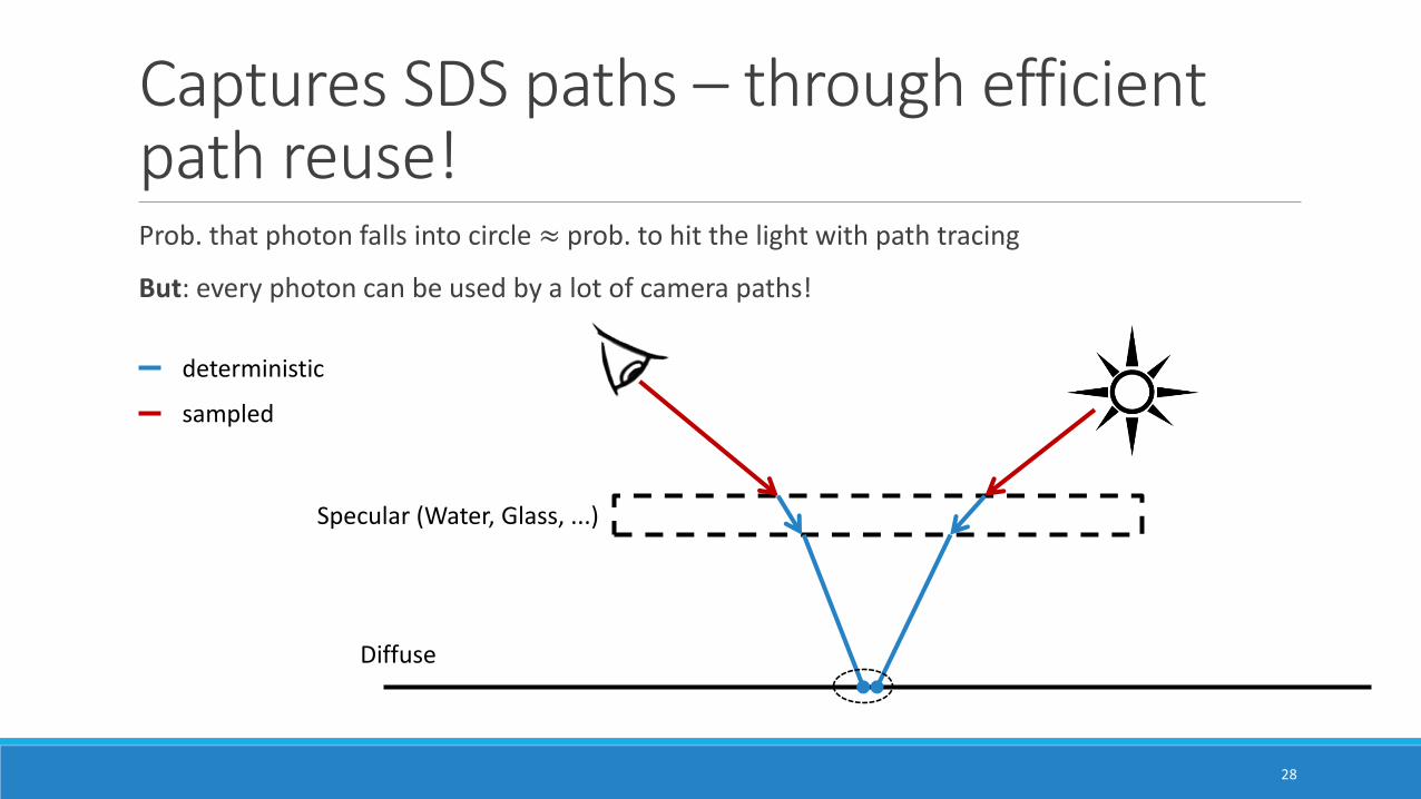
Captures SDS paths – through efficient path reuse!Prob. that photon falls into circle ≈ prob. to hit the light with path tracing

But: every photon can be used by a lot of camera paths!

28

Specular (Water, Glass, ...)

Diffuse

deterministic

sampled

Progressive PM captures SDS paths, but high variance on diffuse surfaces

29

BPT

BPT PPM

PPM

Structural Similarity (SSIM)

Photon Mapping – properties + Very efficient for SDS paths

- Performs poorly on glossy surfaces

- Biased (but consistent, if progressive)

- Photon density might be too low if many photons end up in non-visible regions!

30

Vertex Connection and Merging (VCM)[Georgiev et al 2012] also [Hachisuka et al 2012]

Combine BPT with PPM using MIS

31

MIS weights for VCMIdea: Merging can be considered as using Russian Roulette and connect to the previous vertex.

With a given merge radius 𝑟 we can compute the Russian Roulette PDF:

𝑝𝑎𝑐𝑐 = 𝜋𝑟2

When computing the MIS weights, we have to also consider merging at every vertex

In our partial update scheme, this amounts to adding 𝑝𝑎𝑐𝑐 to the partial sum at every bounce

32

Results after 30 seconds

33

PT: no / noisy caustics BPT: only directly visible caustics VCM: all caustics, but still visible bias from the photon map

34

0

2000

4000

6000

8000

10000

12000

14000

16000

0 50 100 150 200 250 300 350

RMSE over time in the Still Life scene

pt bpt ppm vcm

0.5 FPS

1.8 FPS

Which Algorithm to Use in Practice?VCM is robust – handles most types of scenes well

BUT

Memory Requirements

Requires storing all light path vertices (millions)

each at least 64 bytes -> do not fit in the cache anymore!

Many light vertices are not even useful for the scene!

Complexity

Combines multiple sampling techniques, much more complicated than a path tracer

➔ Difficult to implement efficiently, esp. in parallel

35

What did Common Production Renderers Choose?Many pure path tracers,

◦ e.g. Cycles, Arnold, Disney Hyperion…

Some offer VCM (or variations thereof) in addition to path tracing, ◦ Meant to be used only for scenes with caustics

◦ e.g. Pixar RenderMan

Some combine path tracing and light tracing, ◦ Allows directly visible caustics at little extra cost

◦ e.g. NVIDIA IRay

36