HOPF BIFURCATION IN A LOW-DIMENSION SUBCRITICAL

INSTABILITY MODEL

FIZAY-NOAH LEE

Abstract. We discuss center manifold theory and normal form theory and their appli-cations to bifurcation problems that arise in the study of dynamical systems. We use the

developed theory to show that a particular four-dimensional shear flow model parame-

terized by the Reynolds number undergoes a supercritical Hopf bifurcation at a criticalparameter value, giving rise to subcritical instability of the flow.

Contents

1. Introduction 12. The Model 23. Preliminaries 33.1. Center Manifold Theory 33.2. Parameter-Dependent Center Manifold 53.3. Normal Form Theory Applied to the Hopf Bifurcation 64. Application to Model 124.1. Preliminary Transformations 124.2. Cubic Approximation of Center Manifold 134.3. Center Manifold Reduction 134.4. Normal Form Reduction 144.5. Conclusion 15Acknowledgments 17References 17

1. Introduction

In many shear flows, one can detect fully developed turbulence for sufficiently high Reynoldsnumbers1 R despite the fact that the laminar state is linearly stable to small perturbations.Such observations lead to the idea that, for a given shear flow, there exists a critical value δsuch that the laminar state is asymptotically stable only if the energy of the perturbation islower than δ. Quite reasonably, δ is seen to be a function of R, but little is known about therelationship between δ and R other than the fact that for R less than some (undetermined)constant RG, δ is infinite i.e. the laminar state is globally stable. However, with simplified,

1The Reynolds number is a constant (that arises in fluid dynamics) associated with different fluid flows.

Roughly speaking, high Reynolds numbers indicate turbulent flows and low Reynolds numbers indicate laminar

flows.

1

2 FIZAY-NOAH LEE

lower dimensional models, which still capture many essential features of these so-called sub-critical instabilities (or subcritical transitions)2, the task of finding δ as a function of R ismuch more reasonable (Cossu [3]).

In this paper, we analyze a particular four-dimensional model that arises in the study ofthese subcritical transitions to show that a particular “upper-branch” steady state undergoesa supercritical Hopf bifurcation at some R = RC . Prior to the analysis of the model, weintroduce the model in Section 2, and in Sections 3.1 and 3.2, we develop Center ManifoldTheory, which will allow us to reduce the dimension of our model, so that we can study asimpler model. In Section 3.3, we develop Normal Form Theory specifically applied to Hopfbifurcations as a means to analytically derive a criterion for discerning the occurence of aHopf bifurcation. As we will see, the criterion involves the eigenvalues of the linearization ofthe model at the equilibrium point, at the critical parameter value. Furthermore, it involvesa parameter-dependent function (called the first Lyapunov coefficient) whose value at thecritical parameter value partially determines the type of Hopf bifurcation that occurs.

We begin the analysis of the model in Section 4.1 by performing some transformations towrite the model in a form conducive to the application of center manifold theory. In Sections4.2 and 4.3, we approximate the center manifold up to cubic terms and reduce our model totwo dimensions. In Section 4.4, we go through the transformations necessary to get our nowtwo-dimensional system into a form where we can check the two-condition criteria derived viaNormal Form Theory in Section 3.3. Finally, in Section 4.5, we make explicit computationsto verify the two conditions and conclude that our model undergoes a supercritical Hopfbifurcation at a critical Reynolds number RC .

2. The Model

The model to be studied is four dimensional with variables x1, x2, x3, and x4 - all functionsof time. The variable x3 corresponds to the amplitude of streamwise vortices; x2 correspondsto the amplitude of streamwise streaks; x4 corresponds to the amplitude of sinuous pertur-bations of the streaks; and x1 corresponds to the amplitude of the mean shear induced bythese perturbations. Having xi = 0 (i = 1, 2, 3, 4) corresponds to a laminar flow. Otherwise,we have a turbulent flow (at least instantaneously, so long as the values of xi stay non-zero).Explicitly, the model we work with is given by

x = LRx +N(x)(2.1)

where x = (x1, x2, x3, x4)T ∈ R4, and

LR =

−k21/R 0 0 0

0 −k22/R σ2 00 0 −k23/R 00 0 0 −k24/R− σ1

N(x) =

σ1x

24 − σ2x2x3

−σ4x24 + σ2x1x2σ3x

24

(σ4x2 − σ1x1 − σ3x3)x4

.(2.2)

2Here, the term subcritical does not necessarily relate to the same critical parameter value as the term sub-

critical/supercritical (Hopf) bifurcation does. Subcritical instability is a conventional term in fluid dynamics

used to refer to a particular kind of transition to turbulence from the laminar state.

HOPF BIFURCATION IN A LOW-DIMENSION SUBCRITICAL INSTABILITY MODEL 3

Specifically, for model W97, which we are working with, we use the following parametervalues3:

[k1, k2, k3, k4] = [1.57, 2.28, 2.77, 2.67]

[σ1, σ2, σ3, σ4] = [0.31, 1.29, 0.22, 0.68].

It is clear that for all R > 0, the origin (i.e. the laminar flow) is a steady state, and fromthe upper-triangular form of the matrix LR, it is also clear that it is linearly stable to smallperturbations (i.e. locally attracting). Furthermore, solving for zeros of (2.2) reveals thatat R ≈ 106.14 =: RS , there is a saddle-node bifurcation such that for R > RS , there aretwo additional branches of steady states, namely the upper and lower branches (“upper” and“lower” corresponding to the steady states of larger and smaller norm, respectively). Theparameter value of interest is RC ≈ 139.74, where the linearization of the model centered atthe upper branch steady state has a pair of purely imaginary eigenvalues and a conjugatepair of eigenvalues with negative real part.

Remark 2.3. Explicit computation of zeros using a program will reveal that for R > RSthere are actually four non-zero steady state solutions to (2.1). However, one can verify thatthe system has a symmetry with respect to reflection over the x4-axis, and hence the fournon-zero steady states actually come in pairs, each member of a pair being identical to theother except with the opposite sign for the x4 coordinate. There is no loss of generality inrestricting ourselves to the invariant subspace defined by x4 > 0 and just talking about twoout of the four non-zero steady states.

For more information on and further analysis of the model, see Cossu [3].

3. Preliminaries

It has already been shown numerically that at R = RC , a supercritical Hopf bifurcationtakes place for the upper branch steady state (Lebovitz [5]). We aim to show analyticallywhat has been shown numerically. To do so, we employ Center Manifold Theory and NormalForm Theory, which we discuss below.

3.1. Center Manifold Theory. The theory we develop below will allow us to look at ourmodel restricted to an invariant manifold (the center manifold) and allow us to study theresulting lower dimensional model. It is not obvious that studying the restricted systemshould tell us anything about the original model, but as we will see, center manifold theorytells us that, in fact, under certain conditions the dynamics of a system restricted to itscenter manifold are locally equivalent (in a sense to be described in more detail later) to thedyanamics of the original system.

To begin our treatment of the theory, suppose we have a system

w = f(w)(3.1)

such that w ∈ Rn and f is Cr. Furthermore, suppose that f(0) = 0 and Df(0) has nseigenvalues (s for stable) with negative real part and nc = n − ns (c for center) eigenvalueswith zero real part. Observe that we can, through a change of basis, rewrite (3.1) as

x = Ax + fc(x,y)

y = By + fs(x,y)(3.2)

3W97 refers to a shear flow model proposed by Fabian Waleffe in one of his papers from 1997 (Waleffe

[7]). There is also a related, earlier model, W95, proposed by Waleffe in 1995 (Waleffe [6]). Both models are

discussed in Cossu [3].

4 FIZAY-NOAH LEE

where (x,y) ∈ Rnc × Rns , A has eigenvalues with zero real part, B has eigenvalues withnegative real part, and fc and fs are Cr and have no linear terms. Having thus written oursystem in the form (3.2), we can state the following definition:

Definition 3.3. An invariant manifold is called a center manifold for (3.2) if it can locallybe represented as follows

W c(0) = {(x,y) ∈ Rnc × Rns | y = h(x), |x| < δ, h(0) = 0, Dh(0) = 0}(3.4)

for sufficiently small δ > 0.

Observe that the conditions h(0) = 0 and Dh(0) = 0 imply that W c(0) is tangent, at theorigin, to Ec, the generalized eigenspace corresponding to the eigenvalues of (3.2) with zeroreal part.

Now in the theorem below, we get the existence of a center manifold and the property ofcenter manifolds that allows us to reduce the dimension of (3.1) in studying its dynamics.Note that the theorem gives us existence but not uniqueness.

Theorem 3.5. There exists a Cr center manifold for (3.2). Furthermore, system (3.1) istopologically equivalent near the origin to the system

x = Ax + fc(x, h(x))

y = By(3.6)

where A,B and fc are as in (3.2) and h comes from Definition 3.3.

The first part of system (3.6)

x = Ax + fc(x, h(x)), x ∈ Rnc(3.7)

is called the restriction of (3.2) to its center manifold.The theorem tells us that for some neighborhoods U and V of the origin (in Rnc × Rns),

there exists a homeomorphism from U to V such that orbits of (3.2) contained in U aremapped to orbits of (3.6) contained in V in such a way that preserves the direction of time.In other words, the theorem says that the orbital structures of (3.2) and (3.6) are equivalentnear the origin up to some “bending and pulling.” Particularly, equilibrium points and smallamplitude periodic orbits of (3.2) sufficiently close to the origin exist also for system (3.6),and vice-versa. Notice, furthermore, that for system (3.6), all dynamical behaviors along they coordinates decay exponentially as t→∞ so orbits of (3.6) asymptotically approach orbitsof (3.7) (or, to be precise, orbits of (3.7) adjoined with y = 0). So, Theorem 3.5 allows us,when studying a system like (3.2), to focus instead on the lower dimensional system (3.7) tolearn about the local behavior near an equilibrium point.4

Now the problem boils down to actually computing the center manifold or, equivalently,computing the function h as given in Definition 3.3. We do so by making the following ob-servations.

4Perhaps Theorem 3.5 makes it clear why, up to this point, we have assumed that (3.1) has no eigenvalues

with positive real part: having eigenvalues with positive real part would still give us a theorem like Theorem

3.5 except we would have to state that the matrix B has eigenvalues of both negative and positive real part,so dynamics along the y coordinates would no longer be decaying and hence the center manifold would no

longer be attracting. Then the center manifold loses much of its inherent value in that we cannot simply

focus on (3.7) to study the local behavior of (3.2).

HOPF BIFURCATION IN A LOW-DIMENSION SUBCRITICAL INSTABILITY MODEL 5

1) For any (x,y) ∈W c(0), we have

y = h(x).(3.8)

2) Differentiating (3.8) with respect to time, we find that on W c(0) we must have

y = Dh(x)x.(3.9)

Recall from Definition 3.3 that the center manifold is invariant; therefore, we can look at therestriction of (3.2) to it by making the substitution y = h(x):

x = Ax + fc(x, h(x))

y = Bh(x) + fs(x, h(x)), (x,y) ∈W c(0).(3.10)

3) Substituting (3.10) into (3.9) we get

Dh(x)[Ax + fc(x, h(x))] = Bh(x) + fs(x, h(x))(3.11)

or equivalently,

N (h(x)) := Dh(x)[Ax + fc(x, h(x))]−Bh(x) + fs(x, h(x)) = 0.(3.12)

Therefore, solving the differential equation (3.12) would give us the desired function h; how-ever, in most cases the equation is too complex to feasibly solve. So, we have the followingtheorem, which allows us to approximate h up to any desired degree of accuracy.

Theorem 3.13. Let φ : Rnc → Rns be a C1 mapping with φ(0) = Dφ(0) = 0 such thatN (φ(x)) = O(|x|q) as |x| → 0 for some q > 1. Then |h(x)− φ(x)| = O(|x|q) as |x| → 0.

At this point, we make the observation that system (3.1) does not depend on a parameter,whereas system (2.1) does. Below, we discuss how we can use Theorem 3.5 and Theorem 3.13to analyze a parameter dependent system.

3.2. Parameter-Dependent Center Manifold. Suppose we have a parameter-dependentsystem

w = f(w, µ),w ∈ Rn, µ ∈ R(3.14)

where f(0, 0) = 0 and Dfw(0, 0) has nc eigenvalues with zero real part and ns = n − nceigenvalues with negative real part.

For µ = 0, the center manifold theory from above gives us a center manifold (after rewriting(3.14) in its eigenbasis)

W c0 (0) = {(x,y) ∈ Rnc × Rns | y = h(x), |x| < δ, h(0) = 0, Dh(0) = 0}(3.15)

for δ > 0 sufficiently small. However, we would like to study the system as we vary µnear 0, so we treat µ as a variable (that has no dependence on time) and hence study the(n+ 1)-dimensional system

w = f(w, µ)

µ = 0, w ∈ Rn, µ ∈ R.(3.16)

6 FIZAY-NOAH LEE

It is easy to see that system (3.16) has a (nc + 1)-dimensional center manifold. Througha change of basis, we can change system (3.16) into the form5

x = Ax + fc(x,y, µ)

µ = 0

y = By + fs(x,y, µ), x ∈ Rnc , y ∈ Rns , µ ∈ R(3.17)

where A has eigenvalues with zero real part and B has eigenvalues with negative real part,and fc and fs are nonlinear with respect to x,y, µ. Note that since µ is now considered avariable, A and B can be made independent of µ.

Having gone through these coordinate changes, the parameter-dependent center manifoldof (3.17) is given by

W cµ(0) = {(x,y, µ) ∈ Rnc × Rns × R | y = h(x, µ), |x| < δ, |µ| < δ∗, h(0, 0) = 0, Dh(0, 0) = 0}

for δ, δ∗ > 0 sufficiently small.Now, all the theorems from the parameter-free center manifold theory can easily be ex-

tended for parameter-dependent center manifolds by viewing µ as an extra variable: system(3.17) is topologically equivalent, near the origin, to

x = Ax + fc(x, h(x, µ), µ)

µ = 0

y = By.(3.18)

And, for later use, we state below the differential equation whose solution gives us ourparameter-dependent center manifold (cf. 3.12):

N (h(x, µ)) := Dxh(x, µ)[Ax + fc(x, h(x, µ), µ)]−Bh(x, µ) + fs(x, h(x, µ), µ) = 0.(3.19)

3.3. Normal Form Theory Applied to the Hopf Bifurcation. In this section, we de-velop the analytic machinery that we need to show that a two dimensional system satisyfingcertain properties undergoes a Hopf bifurcation. The general method is to use a series ofsmooth variable changes to change the form of our given system into the normal form of theHopf bifurcation - a “simple” system which we know beforehand undergoes a Hopf bifurca-tion. The normal forms of the supercritical and subcritical Hopf bifurcations, respectively,are given below: [

x1x2

]=

[α −11 α

] [x1x2

]−[x1(x21 + x22)x2(x21 + x22)

](3.20)

[x1x2

]=

[α −11 α

] [x1x2

]+

[x1(x21 + x22)x2(x21 + x22)

](3.21)

Solutions to (3.20) and (3.21) are shown in Figures 1 and 2. In both of these examples, α = 0 isthe critical parameter value at which the stability of the origin changes. A supercritical Hopfbifurcation occurs when a limit cycle forms as α goes from negative to positive. A subcriticalHopf bifurcation occurs when a limit cycle forms as α goes from positive to negative. Thestability of the limit cycle depends on the stability of the equilibrium point it surrounds. One

5There may be a concern that going through the change of basis from (3.16) to (3.17) may change the

variable µ from (3.16) in such a way that in our new system (3.17), varying µ would vary more than just µ

in our original system, in which case we are no longer studying the dynamics of (3.16) as just µ varies. Ingeneral, one would expect this to be the case, but in our case, because in (3.16), µ is precisely equal to zero

(i.e. it is independent of time), one can verify that the variable µ does not actually go through any change

through the change of variables. In particular µ from (3.17) is not dependent on w from (3.16).

HOPF BIFURCATION IN A LOW-DIMENSION SUBCRITICAL INSTABILITY MODEL 7

(a) α < 0 (b) α = 0 (c) α > 0

Figure 1. Supercritical Hopf Bifurcation

(a) α < 0 (b) α = 0 (c) α > 0

Figure 2. Subcritical Hopf Bifurcation

can feasibly see that by changing α to −α above, there are a total of four different kindsof Hopf bifurcations each of which is fully characterized by 1) whether a limit appears forα positive or negative and 2) whether the equilbrium point goes from stable to unstable orunstable to stable as α goes from negative to positive.

Now, given a two-dimensional system

x = f(x, µ), x ∈ R2, µ ∈ R(3.22)

with f(0, 0) = 0, we can show that if our system satisfies certain properties, then we can,through a smooth change of coordinates, transform system (3.22) into the form (3.20) or(3.21), and in doing so we will have shown that the system (3.22) undergoes a Hopf bifurcationat µ = 0.

For the remainder of Section 3, we determine what properties (3.22) must satisfy and whatkinds of changes of coordinates we must use to reduce our system into normal form.

Our first lemma below tells us that if we have a system almost in normal form - almost inthe sense of (3.24) below - then there is a locally defined homeomorphism that maps orbitsof (3.20) (or (3.21)) to orbits of (3.24) for orbits that start sufficiently near the origin. Thismeans that stable (unstable) equilibrium points are mapped to stable (unstable) equilibriumpoints and small amplitude periodic orbits are mapped to periodic orbits. So, our task hasbeen reduced to that of performing the necessary change of coordinates to transform system(3.22) into the form of (3.24).

8 FIZAY-NOAH LEE

Lemma 3.23. The system[x1x2

]=

[α −11 α

] [x1x2

]±[x1(x21 + x22)x2(x21 + x22)

]+O((|x1|+ |x2|)4)(3.24)

is topogically equivalent near the origin to system (3.20) or (3.21) (depending on the sign ofthe cubic terms).

Proof. See Kuznetsov [2]. �

Returning to the task at hand, suppose that in system (3.22), Df(0, 0) has eigenvaluesλ1,2 = ±iω0, ω0 > 0. Then, by the Implicit Function Theorem, for |µ| small enough, wehave a unique equilibrium point x0(µ) ∈ R2 i.e. f(x0(µ), µ) = 0. So by making the changex→ x + x0(µ), we can, for small |µ|, place the equilibrium point at the origin. Having doneso, (3.22) can be written

x = A(µ)x + F (x, µ)(3.25)

where F = O(|x|2). Furthermore, we may assume that we have performed a µ-dependentchange of variables such that for small |µ|, A(µ) is of the form

A(µ) =

[Re(λ(µ)) −Im(λ(µ))Im(λ(µ)) Re(λ(µ))

](3.26)

where λ(µ), λ(µ) are the eigenvalues of Dxf(x, µ)|x=0 for small |µ|.Now we can identity the complex variable z with x1 + ix2, and in doing so can write (3.25)

as a one-dimensional complex system

z = λ(µ)z + g(z, z, µ)(3.27)

where g = O(|z|2). Now observe that system (3.24) can similarly be written in complex form:

z = (α+ i)z ± z|z|2 +O(|z|4).(3.28)

Hence, our goal will be to reduce (3.27) into the form (3.28) through a series of smoothchanges of variables. In doing so, we will have to impose two conditions on (3.27), and hav-ing done so, we will have shown that the system undergoes a Hopf bifurcation at µ = 0 giventhat the two conditions (to be discussed) hold.

We begin the process with the following lemma, which allows us to eliminate all quadraticterms from our system:

Lemma 3.29. The equation

z = λ(µ)z +g20(0, 0, µ)

2z2 + g11(0, 0, µ)zz +

g02(0, 0, µ)

2z2 +O(|z|3)(3.30)

can be transformed by an invertible µ-dependent change of complex coordinates

z = w +h20(µ)

2w2 + h11(µ)ww +

h02(µ)

2w2(3.31)

for all sufficiently small |µ|, into an equation without quadratic terms:

w = λ(µ)w +O(|w|3).(3.32)

Remark 3.33. In the above lemma, we assume gij(0, 0, µ) := ∂i+jg∂zi∂zj

|z=z=0 and λ(µ) =R(µ) + iI(µ), R(0) = 0, I(0) = ω0 > 0. Furthermore note that the subscripts for h do notcorrespond to partial derivatives; hij are smooth functions of µ to be determined. We furtherremark that for the remainder of the paper we will use gij(µ) := gij(0, 0, µ).

HOPF BIFURCATION IN A LOW-DIMENSION SUBCRITICAL INSTABILITY MODEL 9

Proof. (of Lemma 3.29) The inverse change of variables of (3.31) is given by

w = z − h20(µ)

2z2 − h11(µ)zz − h02(µ)

2z2 +O(|z|3)(3.34)

as can be obtained by setting

w = a0 + a1z + a2z + a3z2 + a4zz + a5z

2 +O(|z|3),(3.35)

then substituting (3.35) into (3.31) and solving for the coefficients a0, a1, a2, a3, a4 and a5.Now from (3.34), we get

w = z − h20(µ)zz − h11(µ)(zz + zz)− h02(µ)zz + · · ·(3.36)

Then substituting (3.30) and (3.31) into (3.36) we find (after algebraic manipulations) thatthe constant term on the RHS is zero and the coefficients of w,w,w2, ww, and w2 areλ(µ), 0, 12 (g20(µ) − λ(µ)h20(µ)), g11(µ) − λ(µ)h11(µ), and 1

2 (g02(µ) − (2λ(µ) − λ(µ))h02(µ)),respectively. Thus by setting

h20(µ) =g20(µ)

λ(µ)(3.37)

h11(µ) =g11(µ)

λ(µ)(3.38)

h02(µ) =g02(µ)

2λ(µ)− λ(µ)(3.39)

we get our desired form (3.32). Note that (3.37-39) are well-defined for small |µ| since λ(0) 6= 0by assumption. �

Having thus eliminated the quadratic terms, we attempt to eliminate cubic terms, too:

Lemma 3.40. The equation

z = λ(µ)z +g30(µ)

6z3 +

g21(µ)

2z2z +

g12(µ)

2z2z +

g03(µ)

6z3 +O(|z|4),(3.41)

with the same assumptions as in the previous lemma, can be transformed by an invertibleµ-dependent change of complex coordinates

z = w +h30(µ)

6w3 +

h21(µ)

2w2w +

h12(µ)

2ww2 +

h03(µ)

6w3(3.42)

for all sufficiently small |µ| into an equation with only one cubic term:

w = λ(µ)w + c1(µ)w2w +O(|w|4).(3.43)

Remark 3.44. Observe that we are actually not able to eliminate all cubic terms. The termw2w above is called a resonant term.

Proof. (of Lemma 3.40) The proof of this lemma is essentially identical to that of Lemma3.29. We find by the same method that the inverse change of variables is given by

w = z − h30(µ)

6z3 − h21(µ)

2z2z − h12(µ)

2zz2 − h03(µ)

6z3 +O(|z|4).(3.45)

10 FIZAY-NOAH LEE

Then, by differentiating (3.45) and making the necessary substitutions, we find that by setting

h30(µ) =g30(µ)

2λ(µ)(3.46)

h12(µ) =g12(µ)

2λ(µ)(3.47)

h03(µ) =g03(µ)

3λ(µ)− λ(µ)(3.48)

the coefficients of w3, ww2, w3 all become zero. If we attempt to make the coefficient of w2wzero, then we must set

h21(µ) =g21(µ)

λ(µ) + λ(µ),(3.49)

but we observe that h21(µ) then becomes undefined at µ = 0. Hence we set h21(µ) = 0, whichresults in

c1(µ) =g21(µ)

2.(3.50)

�

Now observe that applying Lemma 3.29 and Lemma 3.40 in succession, we can reduce theequation

z = λ(µ)z +∑

2≤k+l≤3

1

k!l!gkl(µ)zkzl +O(|z|4)(3.51)

into the form (3.43):

w = λ(µ)w + c1(µ)w2w +O(|w|4).

However, note that in first eliminating the quadratic terms, the coefficients of the cubic terms

change, too, so we cannot simply say that c1(µ) = g21(µ)2 . We get around this problem by

doing the following: we can express z in terms of w,w in two ways. First, we can substitute(3.31) into (3.51). Second, since we know that after all the necessary reductions we end upwith an equation of the form (3.43), z can be computed by differentiating (3.31) and thensubstituting in w and w using (3.43). Then, equating the coefficients of w|w|2 (i.e. w2w), weget

c1(µ) =g20(µ)g11(µ)(2λ(µ) + λ(µ))

2|λ(µ)|2+|g11(µ)|2

λ(µ)+

|g02(µ)|2

4λ(µ)− 2λ(µ)+g21(µ)

2.(3.52)

At the critical bifurcation value µ = 0, we have

c1(0) =i

2ω0(g20(0)g11(0)− 2|g11(0)|2 − 1

3|g02(0)|2) +

g21(0)

2.(3.53)

So far, we can reduce an equation of the form (3.51) into the form (3.43):

w = λ(µ)w + c1(µ)w2w +O(|w|4).

Now we would like to transform (3.43) into the normal form discussed previously:

z = (α+ i)z ± z|z|2 +O(|z|4).(3.54)

Lemma 3.55. Given two conditions to be determined, (3.43) can be transformed into theHopf bifurcation normal form (3.54).

HOPF BIFURCATION IN A LOW-DIMENSION SUBCRITICAL INSTABILITY MODEL 11

Proof. Rewrite (3.43) in the following way by setting λ(µ) = R(µ) + iI(µ):

dw

dt= (R(µ) + iI(µ))w + c1(µ)w|w|2 +O(|w|4).(3.56)

By assumption R(0) = 0 and I(0) = ω0 > 0. Now, introduce the µ-dependent time variableτ = I(µ)t. The time direction is preserved since I(µ) is positive for sufficiently small |µ|.Also, define β(µ) = R(µ)

I(µ) . Then, if we impose the condition that R′(0) 6= 0, we have

β(0) = 0, β′(0) =I(0)R′(0)−R(0)I ′(0)

I2(0)=R′(0)

I(0)6= 0.

Hence we can consider β as our new parameter and write µ as a function of β for small |β|,µ = µ(β). So now with the new time variable and new parameter, (3.56) turns into

dw

dτ= (β + i)w + d1(β)w|w|2 +O(|w|4)(3.57)

where d1(β) = c1(µ(β))I(µ(β)) .

We now introduce a new time parameterization along orbits of (3.57), θ = θ(τ, β), where

dθ = (1 + Im(d1(β))|w|2)dτ.(3.58)

With this new definition of time, (3.57) becomes

dw

dθ= (β + i)w + l1(β)w|w|2 +O(|w|4)(3.59)

where l1(β) = Re(d1(β))− β · Im(d1(β)) and

l1(0) =Re(c1(0))

ω0(3.60)

It is not a particularly illuminating process going from (3.57) to (3.59), but one can easilyverify the result by multiplying the RHS of (3.59) by 1 + Im(d1(β))|w|2 to check it results inthe RHS of (3.57).

Finally, if we impose the condition that Re(c1(0)) 6= 0, then l0(0) 6= 0, so we can introducea new complex variable u:

w =u√|l1(β)|

.(3.61)

With this new complex variable, (3.59) becomes

du

dθ= (β + i)u+

l1(β)

|l1(β)|u|u|2 +O(|u|4)

= (β + i)u+ su|u|2 +O(|u|4)(3.62)

where s = l1(0)|l1(0)| = sign l1(0) = sign Re(c1(0)).

This completes the proof. �

Remark 3.63. The real function l1(β) is called the first Lyapunov coefficient. Observe thatfrom (3.53) and (3.60), it follows that the first Lyapunov coefficient evaluated at β = 0 isgiven by

l1(0) =1

2ω20

Re(ig20(0)g11(0) + ω0g21(0)).(3.64)

We summarize Lemma 3.23, Lemma 3.29, Lemma 3.40 and Lemma 3.55 in one theorembelow, making sure to include the two conditions that we imposed in the process:

12 FIZAY-NOAH LEE

Theorem 3.65. Suppose we have a complex system

z = λ(µ)z + g(z, z, µ)(3.66)

where g = O(|z|2) is a smooth function of (z, z, µ) such that g(0, 0, 0) = 0, λ(µ) is a smoothfunction of µ and λ(0) = iω0 (ω0 > 0). Then (3.66) can be reduced to the form (3.62) if thefollowing two conditions hold:

(1) ddµRe(λ(µ))|µ=0 6= 0

(2) The first Lyapunov coefficient evaluated at 0 (given by the formula (3.64)) is nonzero.

Finally from an application standpoint, we have (due to Lemma 3.23):

Corollary 3.67. Given a two-dimensional, parameter-depedent system

x = f(x, µ)(3.68)

with smooth f , having at µ = 0 the equilibrium x = 0 with Df(0, 0) having eigenvaluesλ1,2 = ±iω0, ω0 > 0, the system undergoes a Hopf bifurcation around the origin as µ crosseszero provided the two conditions from Theorem 3.65 hold.

Remark 3.69. Note, however, that to check the conditions, one must first get (3.68) intothe form (3.66) (see text following Lemma 3.23). Furthermore, observe that whether theHopf bifurcation is supercritical or subcritical depends on the sign of the first Lyapunov firstcoefficient evaluated at zero. Whether the periodic solutions are stable or unstable dependson the sign of d

dµRe(λ(µ))|µ=0.

4. Application to Model

Now we are ready to analyze our shear flow model. We begin by adjoining the fourdimensional model with R = 0, making it into a five dimensional system. This allows us toinvestigate the dynamics of our model as our parameter R varies. Then we make the necessarytransformations to set up for the application of center manifold theory. Then, applying thetheory, we reduce our system to two dimensions and, after applying further transformationsto turn our system into the form (3.25), we introduce a complex variable, resulting in a one-dimensional complex system. At this point, we can check our two conditions from Theorem3.65 to verify the occurence of a supercritical Hopf bifurcation.

4.1. Preliminary Transformations. Recall that our model is given by

x = LRx +N(x)(4.1)

where

LR =

−k21/R 0 0 0

0 −k22/R σ2 00 0 −k23/R 00 0 0 −k24/R− σ1

N(x) =

σ1x

24 − σ2x2x3

−σ4x24 + σ2x1x2σ3x

24

(σ4x2 − σ1x1 − σ3x3)x4

(4.2)

with constants

[k1, k2, k3, k4] = [1.57, 2.28, 2.77, 2.67]

[σ1, σ2, σ3, σ4] = [0.31, 1.29, 0.22, 0.68].

HOPF BIFURCATION IN A LOW-DIMENSION SUBCRITICAL INSTABILITY MODEL 13

Since we are studying the dynamics of (4.1) as R varies near the critical value, we adjoin

R = 0 (cf. Section 3.2). Now, we recall that our critical bifurcation value is given byRC ≈ 139.74, where the linearization of (4.1) at the equilibrium point (x∗1 ≈ −0.8015, x∗2 ≈0.1923, x∗3 ≈ 0.0828, x∗4 ≈ 0.1438) has two eigenvalues with negative real part (−a ± bi,a, b > 0) and two eigenvalues with zero real part (±iω, ω > 0).

For convenience, we make the linear shifts to move the equilbrium point in question to theorigin. Furthermore, we make the change of variables r′ = 1/R, and then r = r′ − 1/RC , sothat now, with r as the parameter, we can view our system as being made up of polynomialsin x1, x2, x3, x4 and r, where r = 0 is the critical bifurcation value. Also, note the inverserelation of r and R: this will be necessary for the interpretation of results later on.

So, starting with the five-dimensional system

x = LRx +N(x)

R = 0.(4.3)

we perform the changes of variables mentioned in the previous paragraph and then rewritethe resulting system in real canonical form, resulting in the system

x1x2x3x4r

=

−a −b 0 0 0b −a 0 0 00 0 0 −ω 00 0 ω 0 00 0 0 0 0

x1x2x3x4r

+

N∗1 (x1, x2, x3, x4, r)N∗2 (x1, x2, x3, x4, r)N∗3 (x1, x2, x3, x4, r)N∗4 (x1, x2, x3, x4, r)

0

(4.4)

where N∗i are nonlinear with respect to x1, x2, x3, x4, r.

4.2. Cubic Approximation of Center Manifold. Now we can apply the center manifoldtheorem to find the restriction of our system to its center manifold. We begin by approximat-ing the center manifold of (4.4) at the equilibrium point (0,0,0,0,0). Notice that the centermanifold in our case is three dimensional, and the theorem gives us two smooth functionsx1 = h1(x3, x4, r) and x2 = h2(x3, x4, r) whose graph near the origin of (x1, x2, x3, x4, r)-spacegives us our center manifold. At this point, we use Theorem 3.13 to approximate our twofunctions. For our purposes, it is sufficient to approximate h1(x3, x4, r) and h2(x3, x4, r) up tocubic terms.6 From center manifold theory, we also know hi(0, 0, 0) = 0 and Dhi(0, 0, 0) = 0,hence we can write our functions as

hi(x3, x4, r) =ai1x23 + ai2x

24 + ai3r

2 + ai4x3x4 + ai5x3r + ai6x4r

ai7x33 + ai8x

34 + ai9r

3 + ai10x23x4 + ai11x3x

24

+ ai12x23r + ai13x3r

2 + ai14x24r + ai15x4r

2

+ ai16x3x4r +O((|x3|+ |x4|+ |r|)4)(4.5)

for i = 1, 2 where the coefficients are currently unknown. We solve for the coefficients aijusing the fact that hi(x3, x4, r) must satisfy (cf. 3.19)

D

[h1h2

][

[0 −ωω 0

] [x3x4

]+

[N∗3 (h1, h2, x3, x4, r)N∗4 (h1, h2, x3, x4, r)

]]

−[−a −bb −a

] [h1h2

]+

[N∗1 (h1, h2, x3, x4, r)N∗2 (h1, h2, x3, x4, r)

]= 0(4.6)

where the derivative D is with respect to x3 and x4, and h1 and h2 are functions of x3, x4, r.Substituting (4.5) into (4.6) and setting the coefficients of all the quadratic and cubic

6This statement is justified by Lemma 3.23.

14 FIZAY-NOAH LEE

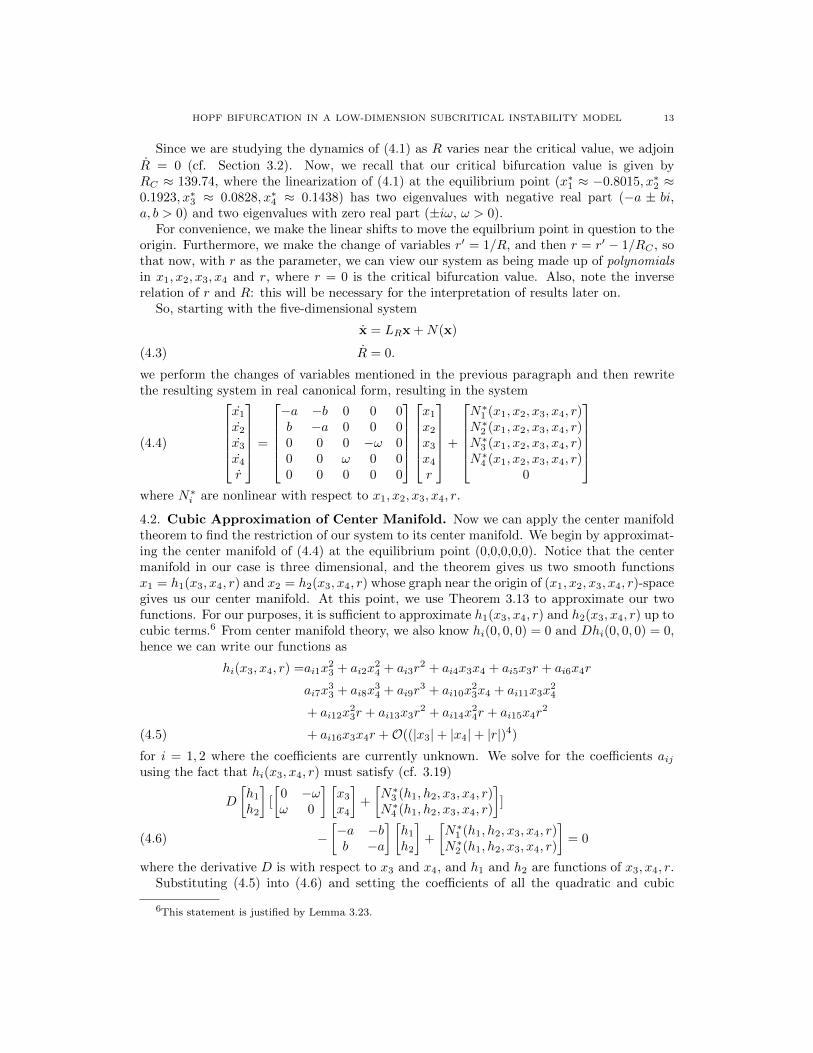
(a) r < 0 (b) r = 0 (c) r > 0

Figure 3. System (4.7)

terms equal to zero, we get a unique real solution set for aij , where i = 1, 2, j = 1, ..., 16.Thus, by Theorem 3.13, we have obtained approximations whose difference with the actualfunctions h1 and h2 is O((|x3|+ |x4|+ |r|)4). For the remainder of the paper, we will call theapproximating functions h1 and h2.

4.3. Center Manifold Reduction. Now as a direct application of center manifold theory,we can simply study our system (4.4) restricted to its center manifold (cf. 3.7) to study thedynamics of (4.4) near the origin as r is varied near 0.

The restriction to the center manifold is given by[x3x4

]=

[0 −ωω 0

] [x3x4

]+

[N∗3 (h1, h2, x3, x4, r)N∗4 (h1, h2, x3, x4, r)

]r = 0.

Notice, however, that there are no dynamics along the r-axis, and hence we need only focuson the system[

x3x4

]=

[0 −ωω 0

] [x3x4

]+

[N∗3 (h1, h2, x3, x4, r)N∗4 (h1, h2, x3, x4, r)

]=:

[F3(x3, x4, r)F4(x3, x4, r)

].(4.7)

Before proceeding, we can use a program to graph the above system (Figure 3).Just based on the plots from Figure 3, one can see that as r goes from negative to

positive, the equilibrium goes from stable to unstable, and comparing the red and orangeorbits in (A), one can see that a periodic orbit should exist somewhere “in between” thosetwo orbits. However, for r > 0, all orbits are leaving the equilibrium and there is no periodicsolution. Thus, we have at least graphically verified the occurence of a (subcritical) Hopfbifurcation at r = 0.

4.4. Normal Form Reduction. Now, to actually apply the theory from Section 3.3, wemust get system (4.7) in the form (3.66):

z = λ(µ)z + g(z, z, µ).

We recall, however, that in order to make the transformation to the form (3.66), it is necessaryto make a r-dependent coordinate change such that for all small |r|, we have F3(0, 0, r) =F4(0, 0, r) = 0. This is done by observing that[

F3(0, 0, 0)F4(0, 0, 0)

]= 0

HOPF BIFURCATION IN A LOW-DIMENSION SUBCRITICAL INSTABILITY MODEL 15

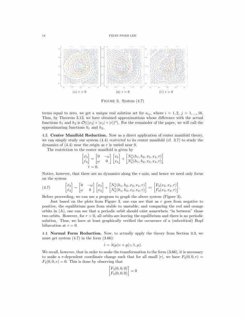
(a) x∗3(r) (b) x∗4(r)

Figure 4

and the Jacobian of

[F3(x3, x4, r)F4(x3, x4, r)

]with respect to x3, x4 evaluated at (0, 0, 0) is invertible.

Hence, it is theoretically possible to write x3 and x4 as functions of r near the origin. Thatis, we have functions

x3 = x∗3(r)

x4 = x∗4(r)(4.8)

such that F3(x∗3(r), x∗4(r), r) = F4(x∗3(r), x∗4(r), r) = 0 for all small |r|. In practice, we canuse a program to find x∗i (r) at sufficiently many points r and then interpolate to acquire afunction that is “correct” up to high orders. For this model, we restricted ourselves to thedomain r ∈ (−0.1, 0.1) and interpolation resulted in functions x∗3(r) and x∗4(r) as shown inFigure 4.

Now making the variable changes x3 7→ x3 − x∗3(r) and x4 7→ x4 − x∗4(r), (4.7) turns into[x3x4

]=

[G3(x3, x4, r)G4(x3, x4, r)

](4.9)

where (0, 0, r) is an equilibrium point for all small |r|. We can try graphing (4.9) at thisintermediate stage, but because x∗3,4(r) is very small for small |r|, one will see that theresulting plots are visually almost indistinguishable from Figure 3. In particular, all theobservations we made for the graphs of system (4.7) still hold for system (4.9).

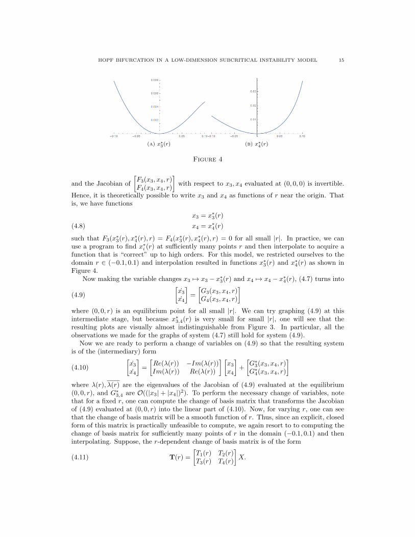
Now we are ready to perform a change of variables on (4.9) so that the resulting systemis of the (intermediary) form[

x3x4

]=

[Re(λ(r)) −Im(λ(r))Im(λ(r)) Re(λ(r))

] [x3x4

]+

[G∗3(x3, x4, r)G∗4(x3, x4, r)

](4.10)

where λ(r), λ(r) are the eigenvalues of the Jacobian of (4.9) evaluated at the equilibrium(0, 0, r), and G∗3,4 are O((|x3| + |x4|)2). To perform the necessary change of variables, notethat for a fixed r, one can compute the change of basis matrix that transforms the Jacobianof (4.9) evaluated at (0, 0, r) into the linear part of (4.10). Now, for varying r, one can seethat the change of basis matrix will be a smooth function of r. Thus, since an explicit, closedform of this matrix is practically unfeasible to compute, we again resort to to computing thechange of basis matrix for sufficiently many points of r in the domain (−0.1, 0.1) and theninterpolating. Suppose, the r-dependent change of basis matrix is of the form

T(r) =

[T1(r) T2(r)T3(r) T4(r)

]X.(4.11)

16 FIZAY-NOAH LEE

(a) Re(T1(r)) (b) Re(T2(r))

(c) Re(T3(r)) (d) Re(T4(r))

Figure 5. Real Parts of Ti

(a) Im(T1(r)) (b) Im(T2(r))

(c) Im(T3(r)) (d) Im(T4(r))

Figure 6. Imaginary Parts of Ti

where X is the constant 2 × 2 change of basis matrix that transforms a matrix in the Jordancanonical form into the real canonical form. Then, by the process described above, we obtainfunctions Ti(r), whose real and imaginary parts we plot separately in Figures 5 and 6.

Now using the transformation given by T(r), we can transform (4.9) into the form

HOPF BIFURCATION IN A LOW-DIMENSION SUBCRITICAL INSTABILITY MODEL 17

(a) r < 0 (b) r = 0 (c) r > 0

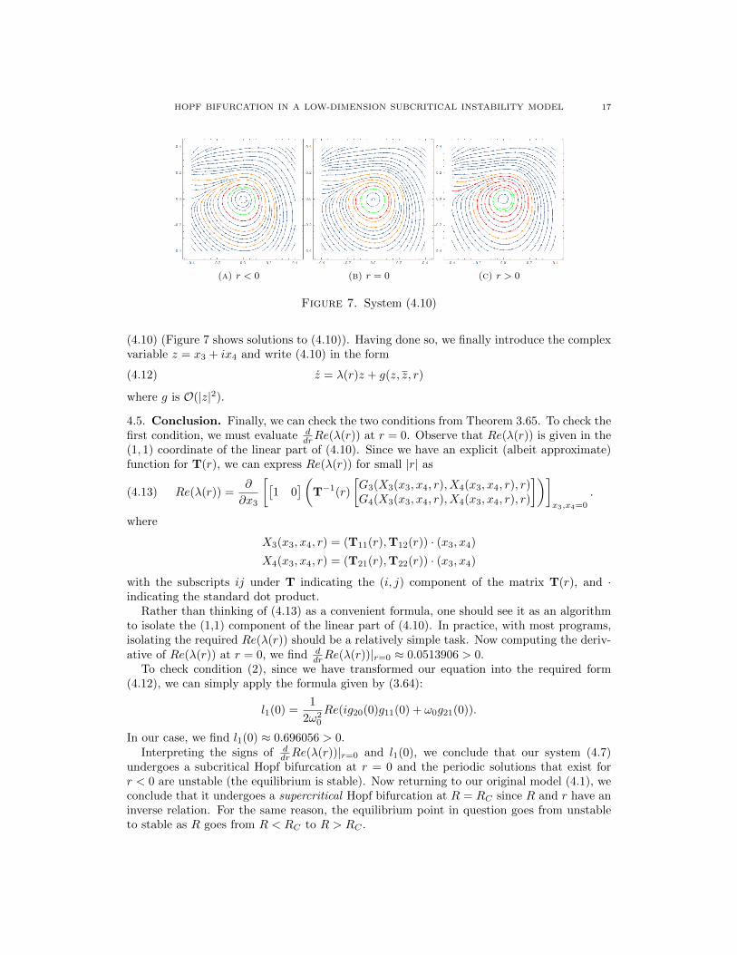
Figure 7. System (4.10)

(4.10) (Figure 7 shows solutions to (4.10)). Having done so, we finally introduce the complexvariable z = x3 + ix4 and write (4.10) in the form

z = λ(r)z + g(z, z, r)(4.12)

where g is O(|z|2).

4.5. Conclusion. Finally, we can check the two conditions from Theorem 3.65. To check thefirst condition, we must evaluate d

drRe(λ(r)) at r = 0. Observe that Re(λ(r)) is given in the(1, 1) coordinate of the linear part of (4.10). Since we have an explicit (albeit approximate)function for T(r), we can express Re(λ(r)) for small |r| as

Re(λ(r)) =∂

∂x3

[[1 0

](T−1(r)

[G3(X3(x3, x4, r), X4(x3, x4, r), r)G4(X3(x3, x4, r), X4(x3, x4, r), r)

])]x3,x4=0

.(4.13)

where

X3(x3, x4, r) = (T11(r),T12(r)) · (x3, x4)

X4(x3, x4, r) = (T21(r),T22(r)) · (x3, x4)

with the subscripts ij under T indicating the (i, j) component of the matrix T(r), and ·indicating the standard dot product.

Rather than thinking of (4.13) as a convenient formula, one should see it as an algorithmto isolate the (1,1) component of the linear part of (4.10). In practice, with most programs,isolating the required Re(λ(r)) should be a relatively simple task. Now computing the deriv-ative of Re(λ(r)) at r = 0, we find d

drRe(λ(r))|r=0 ≈ 0.0513906 > 0.To check condition (2), since we have transformed our equation into the required form

(4.12), we can simply apply the formula given by (3.64):

l1(0) =1

2ω20

Re(ig20(0)g11(0) + ω0g21(0)).

In our case, we find l1(0) ≈ 0.696056 > 0.Interpreting the signs of d

drRe(λ(r))|r=0 and l1(0), we conclude that our system (4.7)undergoes a subcritical Hopf bifurcation at r = 0 and the periodic solutions that exist forr < 0 are unstable (the equilibrium is stable). Now returning to our original model (4.1), weconclude that it undergoes a supercritical Hopf bifurcation at R = RC since R and r have aninverse relation. For the same reason, the equilibrium point in question goes from unstableto stable as R goes from R < RC to R > RC .

18 FIZAY-NOAH LEE

Acknowledgments

I would like to thank Professor Lebovitz for suggesting this topic for me to study and forhis continuous guidance and assistance in completing this project. Also, I would like to thankMary He for her valuable feedback and her willingness to meet up and discuss the material.Last but not least, I thank Professor May for organizing this REU and for giving me and allthe other students this opportunity to study more math.

References

[1] Wiggins, Stephen. Introduction to Applied Nonlinear Dynamical Systems and Chaos. 2nd ed. New York:Springer, 2003. Print.

[2] Kuznetsov, Yuri A. Elements of Applied Bifurcation Theory. 2nd ed. New York: Springer, 1998. Print.[3] Cossu, Carlo. “An Optimality Condition on the Minimum Energy Threshold in Subcritical Instabilities.”

Comptes Rendus Mcanique 333.4 (2005): 331-36. Web.

[4] Carr, Jack. Applications of Centre Manifold Theory. New York: Springer-Verlag, 1981. Print.[5] Lebovitz, Norman, and Giulio Mariotti. “Edges in Models of Shear Flow.” J. Fluid Mech. Journal of Fluid

Mechanics 721 (2013): 386-402. Web.

[6] Waleffe, Fabian.“Transition in Shear Flows. Nonlinear Normality versus Non-normal Linearity.” Physicsof Fluids Phys. Fluids 7.12 (1995): 3060. Web.

[7] Waleffe, Fabian. “On a Self-sustaining Process in Shear Flows.” Physics of Fluids Phys. Fluids 9.4 (1997):

883. Web.