Horizontally Explicit and Vertically Implicit (HEVI) Time Discretization Scheme for a Discontinuous Galerkin Nonhydrostatic Model LEI BAO Department of Applied Mathematics, University of Colorado Boulder, Boulder, Colorado ROBERT KLÖFKORN AND RAMACHANDRAN D. NAIR National Center for Atmospheric Research,* Boulder, Colorado (Manuscript received 25 March 2014, in final form 23 October 2014) ABSTRACT A two-dimensional nonhydrostatic (NH) atmospheric model based on the compressible Euler system has been developed in the (x, z) Cartesian domain. The spatial discretization is based on a nodal discontinuous Galerkin (DG) method with exact integration. The orography is handled by the terrain-following height- based coordinate system. The time integration uses the horizontally explicit and vertically implicit (HEVI) time-splitting scheme, which is introduced to address the stringent restriction on the explicit time step size due to a high aspect ratio between the horizontal (x) and vertical (z) spatial discretization. The HEVI scheme is generally based on the Strang-type operator-split approach, where the horizontally propagating waves in the Euler system are solved explicitly while the vertically propagating waves are treated implicitly. As a conse- quence, the HEVI scheme relaxes the maximum allowed time step to be mainly determined by the horizontal grid spacing. The accuracy of the HEVI scheme is rigorously compared against that of the explicit strong stability-preserving (SSP) Runge–Kutta (RK) scheme using several NH benchmark test cases. The HEVI scheme shows a second-order temporal convergence, as expected. The results of the HEVI scheme are qualitatively comparable to those of the SSP-RK3 scheme. Moreover, the HEVI DG formulation can also be seamlessly extended to account for the second-order diffusion as in the case of the standard SSP-RK DG formulation. In the presence of orography, the HEVI scheme produces high quality results, which are visually identical to those produced by the SSP-RK3 scheme. 1. Introduction With an increased amount of supercomputing resources available to present-day modelers, it is possible to develop global atmospheric models with horizontal grid resolution of the order of a few kilometers. At this fine resolution, the models require a set of nonhydrostatic (NH) govern- ing equations in order to resolve clouds at a global scale (Tomita et al. 2008). However, this necessitates the de- velopment of spatial and temporal discretization schemes that are capable of facilitating excellent parallel efficiency on peta-scale computers. Numerical schemes that can ad- dress these challenges should have computationally desir- able local properties such as compact computational stencils, high on-processor operations, and minimal communica- tion footprints. There is a renewed interest in developing new NH models based on finite-volume (FV; Ahmad and Linedman 2007; Norman et al. 2011; Skamarock et al. 2012; Ullrich and Jablonowski 2012; Li et al. 2013) and Galerkin methods (Giraldo and Restelli 2008; Giraldo et al. 2013; Brdar et al. 2013), which are designed to ad- dress these computational challenges to a great extent. Among the emerging approaches for spatial discretiza- tion, the discontinuous Galerkin (DG) method stands out as a strong candidate, owing to its several computationally attractive features such as local and global conservation, high-order accuracy, high parallel efficiency, and geo- metric flexibility. The DG method may be viewed as a hybrid approach combining the desirable features of two standard numerical discretization approaches: FV * The National Center for Atmospheric Research is sponsored by the National Science Foundation. Corresponding author address: R. D. Nair, Computational and Information System Laboratory, National Center for Atmospheric Research, Boulder, CO 80305. E-mail: [email protected]972 MONTHLY WEATHER REVIEW VOLUME 143 DOI: 10.1175/MWR-D-14-00083.1 Ó 2015 American Meteorological Society
Transcript
Horizontally Explicit and Vertically Implicit (HEVI) Time DiscretizationScheme for a Discontinuous Galerkin Nonhydrostatic Model
LEI BAO
Department of Applied Mathematics, University of Colorado Boulder, Boulder, Colorado
ROBERT KLÖFKORN AND RAMACHANDRAN D. NAIR
National Center for Atmospheric Research,* Boulder, Colorado
(Manuscript received 25 March 2014, in final form 23 October 2014)
ABSTRACT
A two-dimensional nonhydrostatic (NH) atmospheric model based on the compressible Euler system has
been developed in the (x, z) Cartesian domain. The spatial discretization is based on a nodal discontinuous
Galerkin (DG) method with exact integration. The orography is handled by the terrain-following height-
based coordinate system. The time integration uses the horizontally explicit and vertically implicit (HEVI)
time-splitting scheme, which is introduced to address the stringent restriction on the explicit time step size due
to a high aspect ratio between the horizontal (x) and vertical (z) spatial discretization. The HEVI scheme is
generally based on the Strang-type operator-split approach, where the horizontally propagating waves in the
Euler system are solved explicitly while the vertically propagating waves are treated implicitly. As a conse-
quence, the HEVI scheme relaxes the maximum allowed time step to be mainly determined by the horizontal
grid spacing. The accuracy of the HEVI scheme is rigorously compared against that of the explicit strong
stability-preserving (SSP) Runge–Kutta (RK) scheme using several NH benchmark test cases. The HEVI
scheme shows a second-order temporal convergence, as expected. The results of the HEVI scheme are
qualitatively comparable to those of the SSP-RK3 scheme. Moreover, the HEVI DG formulation can also be
seamlessly extended to account for the second-order diffusion as in the case of the standard SSP-RK DG
formulation. In the presence of orography, theHEVI scheme produces high quality results, which are visually
identical to those produced by the SSP-RK3 scheme.
1. Introduction
With an increased amount of supercomputing resources
available to present-daymodelers, it is possible to develop
global atmosphericmodels with horizontal grid resolution
of the order of a few kilometers. At this fine resolution,
the models require a set of nonhydrostatic (NH) govern-
ing equations in order to resolve clouds at a global scale
(Tomita et al. 2008). However, this necessitates the de-
velopment of spatial and temporal discretization schemes
that are capable of facilitating excellent parallel efficiency
on peta-scale computers. Numerical schemes that can ad-
dress these challenges should have computationally desir-
able localproperties such as compact computational stencils,
high on-processor operations, and minimal communica-
tion footprints. There is a renewed interest in developing
newNHmodels based on finite-volume (FV; Ahmad and
Linedman 2007; Norman et al. 2011; Skamarock et al.
2012; Ullrich and Jablonowski 2012; Li et al. 2013) and
Galerkin methods (Giraldo and Restelli 2008; Giraldo
et al. 2013; Brdar et al. 2013), which are designed to ad-
dress these computational challenges to a great extent.
Among the emerging approaches for spatial discretiza-
tion, the discontinuous Galerkin (DG) method stands out
as a strong candidate, owing to its several computationally
attractive features such as local and global conservation,
high-order accuracy, high parallel efficiency, and geo-
metric flexibility. The DG method may be viewed as
a hybrid approach combining the desirable features of
two standard numerical discretization approaches: FV
*The National Center for Atmospheric Research is sponsored
by the National Science Foundation.
Corresponding author address: R. D. Nair, Computational and
Information System Laboratory, National Center for Atmospheric
we choose SSP-RK3 as the explicit time integrator for the
horizontal direction (33) and we solve the vertical di-
rection (34) either with the explicit RKmethod SSP-RK2,
which leads to an horizontal explicit and vertical explicit
(HEVE) method, for comparison studies, or with an im-
plicit time stepping method DIRK2, which is our HEVI
scheme. Therefore, the time integration schemes studied
in the present paper are given as follows:
HEVI (or HEVE) time integrator
1) Solve (36) via SSP-RK3,
2) Solve (37) via DIRK2 (or SSP-RK2), and
3) Solve (38) via SSP-RK3.
The introduction of the HEVE time integration
scheme is solely for the purpose of validating the idea of
dimensional splitting for DG methods and, in practice,
we would adopt the HEVI scheme for practical appli-
cations. When using an implicit method for the vertical
direction (34), it is observed that the CFL condition for
the whole system may be relaxed to the CFL condition
for the horizontal part only. In other words, Dt for theStrang-splitting can be chosen as the largest possible Dtof (33). In this way, the overall performance can be greatly
accelerated. Nevertheless, the necessity of solving an im-
plicit system introduces an additional overhead. In terms
of the performance of the DIRK methods, usually the
number of Newton iterations is very small (i.e., 1 or 2 and
usually not higher than 5). Therefore, the performance of
the implicit solver is closely related to the number of it-
erations of the linear solver. This can be reduced by proper
preconditioning. However, in the current implementation,
no preconditioning is applied. The construction of a proper
preconditioning method is ongoing work. In addition, be-
cause of our domain decomposition, we obtain an implicit
system for each vertical column,which is decoupled for the
other column systems. Therefore, no communication is
needed for the implicit solvers. Even a direct solver could
be applied since the system for one column is not that
large. This will overcome the need for preconditioning
the iterative solvers used otherwise.
The existing IMEXschemes (Ascher et al. 1997;Giraldo
et al. 2013) can be easily incorporated into the HEVI-DG
framework, which may yield some beneficial properties.
To apply an IMEX time integrator, we first rewrite our
problem such that we distinguish between a part that
should be treated implicitly, here Lim, and a part that
should be treated explicitly, here Lex, such that
d
dtUh 5Lim(Uh)1Lex(Uh) in (tn, tn11] . (40)
For the IMEX RK method, we define f im[U(t), t] 5Lim[U(t)] and f ex[U(t), t]5 Lex[U(t)]. The performance
of IMEX schemes combined with DG spatial dis-
cretization may be revisited in a future study.
5. Numerical experiments
To demonstrate and evaluate theHEVI time integration
scheme in the DG-NHmodel, we choose several standard
benchmark tests from the literature. Before detailing with
each test case, we briefly discuss some common features
such as the grid resolution, boundary conditions, and the
initialization process used in the DG-NH model.
a. Numerical experiments setup
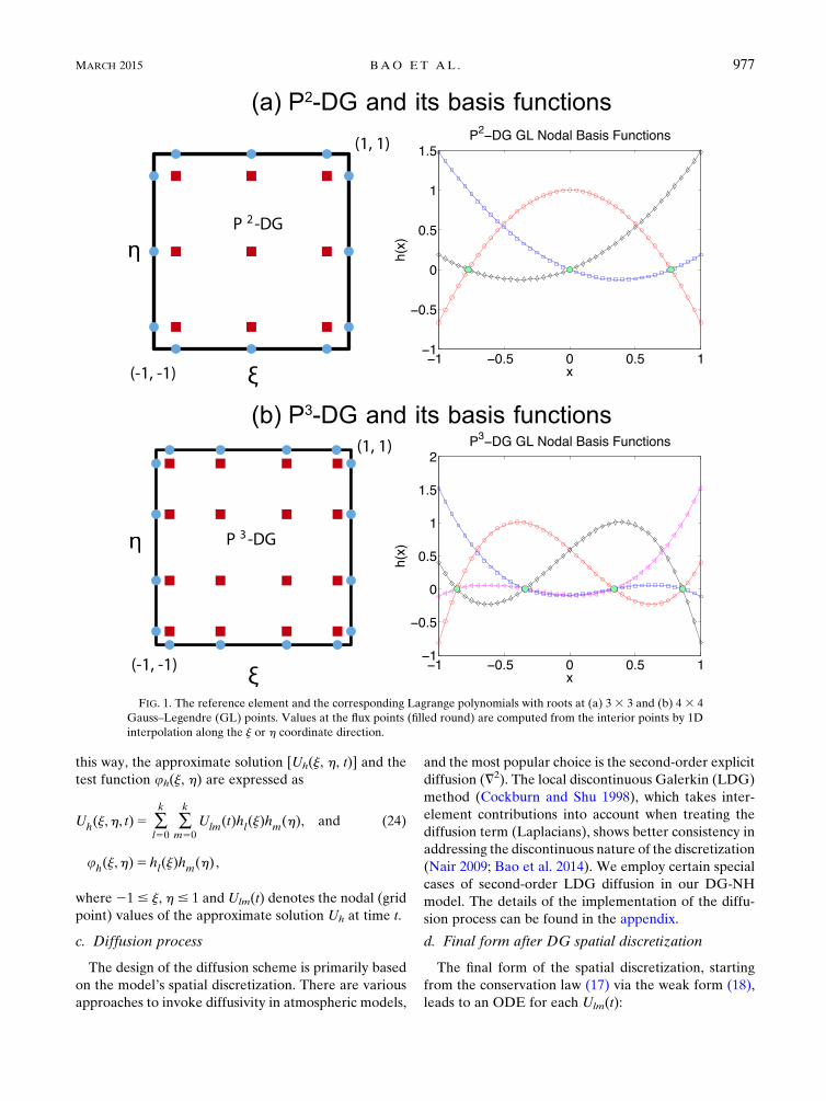
The spatial resolution should take account of the grid
spacing within each element for the nodal DG (RK-DG)
method. For the GL case, the edge points of each ele-
ment are not included as solution points (see Fig. 1);
therefore, we use an approximate procedure to define
the minimum grid spacing for the Pk-DGmethod, which
has k 1 1 degrees of freedom (dof) in each direction.
The average grid spacing is defined in terms of dof as
Dx5Dxi/(k1 1), Dz5Dzj/(k1 1), (41)
where Dxi and Dzj are the element width in the x di-
rection and z direction, respectively [(21) and (22)]. We
employ uniform elements over the whole domain, and
use this convention in (41) as the grid resolution in our
DG-NH model. Note that our definition of grid spacing
is similar to Brdar et al. (2013) but different from that of
Giraldo andRestelli (2008), where they use theGLLgrid.
The DG-NH model, designed for a rectangular domain,
requires suitable boundary conditions for various test
cases. These include no-flux, periodic, and nonreflecting
type boundary specifications.
1) NO-FLUX BOUNDARY CONDITIONS
Essentially, the no-flux (or reflecting) boundary con-
ditions eliminate the normal velocity component to the
980 MONTHLY WEATHER REV IEW VOLUME 143
boundary and only keep the tangential component. For
an arbitrary velocity vector v, the no-flux boundary
condition results in v � n 5 0, where n is the outdrawn
normal vector from the boundary. We denote (yk, y?) asthe parallel (tangential) and perpendicular (normal)
components, respectively, of v along the boundary wall;
let the left and right values at the element edge of v
along the boundary be yL and yR, respectively. Then the
no-flux boundary conditions can be written in the fol-
lowing form:
y?R 52y?L , ykR 5 y
kL . (42)
The same idea is used for the flux vectors along the
boundary.
2) NONREFLECTING BOUNDARY CONDITIONS
The nonreflecting (or transparent) boundary condi-
tions are used to prevent the reflected waves from
reentering the domain, which may interfere or pollute
the flow structure. For the mountain test cases, non-
reflecting boundary conditions are commonly imposed
at the top (zT) and the lateral boundaries, by introducing
the sponge (absorbing) layers of finite width as discussed
in Durran and Klemp (1983). We use a simple damping
function as given below, and the damping terms will act
as an additional forcing to the governing equations in
(15). The prognostic vector U is then damped by relax-
ing to its initial state U0.
In the presence of orography, the governing equations
become
›U
›t5⋯2 t(x, z)(U2U0) , (43)
where t(x, z) is the sponge function, and at the upper
boundary it is defined as (Melvin et al. 2010)
t(x, z)5
8><>:0, if zT2z$zD,
ttop
�sin
�p
2
jzT2zj2zDzD
��4otherwise,
(44)
where ttop is the specified sponge coefficient and zD is
the thickness of the sponge zone from the domain
boundary zT in the z direction. The sponge function is
accountable for the strength of damping over the zone.
Similarly, for the lateral boundaries sponge functions
can be defined with sponge coefficient tlat. In the overlap
region (top corners), we use the maximum of the co-
efficients in the x and z directions. The damping term in
(44) has no effect on the interior part of the domain.
Note that the magnitude of sponge thickness zD, ttop,
and tlat is model dependent, a choice of which is in fact
a trade-off between computational expense and the
quality of the solution.
3) INITIAL CONDITIONS
For the DG-NH model, we use several standard
conversion formulas for model initialization and main-
tain the hydrostatic balance. To initialize the hydrostatic
balance, we obtain a vertical profile for the Exner
pressure p, which is a function of pressure, given as
p5
�p
p0
�Rd/c
p
, (45)
which follows the hydrostatic balance:
dp
dz52
g
cpu. (46)
For some of the tests, a constant Brunt–Väisälä fre-quency Nf is specified and, therefore, u(z) can be com-
puted from the following formula:
N2f 5 g
d
dz(lnu) 0 u(z)5 u0 exp
N2
f
gz
!, (47)
where u0 is a given constant. Once u(z) is known, the
hydrostatically balanced Exner pressure in (45) can be
derived as below:
p(z)5 11g2
cpu0N2f
"exp
2z
N2f
g
!2 1
#
5 12g2
cpN2f
"u(z)2 u0u(z)u0
#. (48)
Another useful formula for computing r fromp by using
the conversion T5 u(z)/p(z) is
r5p0RdT
p(cp/R
d). (49)
For better visualization, the numerical results obtained
from the DG-NH model simulations on the GL grid are
bilinearly interpolated onto a high-resolution uniform
grid.
b. Idealized NH test cases
We consider several NH benchmark test cases with
varying complexities for validating the DG-NH model
with HEVI time stepping. Except for the first test, all
other test cases have no analytical solution and will,
therefore, be evaluated qualitatively.
MARCH 2015 BAO ET AL . 981
1) TRAVELING SINE-WAVE TEST
To study the convergence of the HEVI scheme, we
consider a test case where an analytical solution is
available for the Euler equations. This test case is de-
scribed in Liska andWendroff (2003), but we use a slight
modification for the velocity and pressure suitable for
our application. This test case simulates the traveling of
sine waves at a nonhydrostatic scale on a square domain
[0, 1] 3 [0, 1]m2, where the waves march along the di-
agonal direction. The constant wind fields u 5 (u0, w0)
are defined as
u0(x, z, t)5 sinp
5, w0(x, z, t)5 cos
p
5. (50)
The pressure p is set to be a constant 0.3 Pa, and the
density is given as follows:
r(x, z, t)5
�0:5 if R. 1:0,0:25fcos[pR(x, z, t)]1 1:0g21 0:5 else,
The initial condition can be obtained by setting t 5 0 s.
Periodic boundary conditions are imposed for all four
boundaries, and the simulation time is tT5 0.1 s. To fit the
governing equations in (15), the hydrostatically balanced
variables (r, p, u) are all set to zero. We neglect the in-
fluence of gravity and set the source term S in (16) to zero.
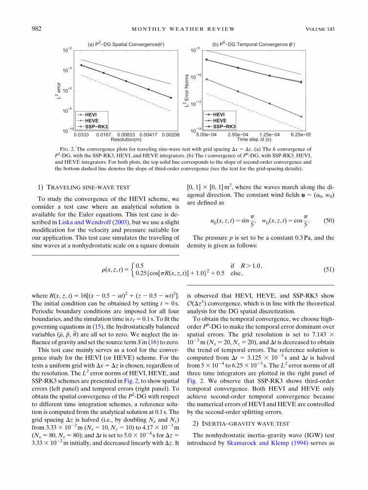
This test case mainly serves as a tool for the conver-
gence study for the HEVI (or HEVE) scheme. For the
tests a uniform grid with Dx5 Dz is chosen, regardless ofthe resolution. TheL2 error norms of HEVI, HEVE, and
SSP-RK3 schemes are presented in Fig. 2, to show spatial
errors (left panel) and temporal errors (right panel). To
obtain the spatial convergence of the P2-DGwith respect
to different time integration schemes, a reference solu-
tion is computed from the analytical solution at 0.1 s. The
grid spacing Dz is halved (i.e., by doubling Nx and Nz)
from 3.333 1022m (Nx 5 10, Nz 5 10) to 4.173 1023m
(Nx 5 80,Nz 5 80); and Dt is set to 5.03 1024 s for Dz53.333 1022m initially, and decreased linearly with Dz. It
is observed that HEVI, HEVE, and SSP-RK3 show
O(Dz3) convergence, which is in line with the theoretical
analysis for the DG spatial discretization.
To obtain the temporal convergence, we choose high-
order P6-DG to make the temporal error dominant over
spatial errors. The grid resolution is set to 7.143 31023m (Nx5 20,Nz5 20), and Dt is decreased to obtain
the trend of temporal errors. The reference solution is
computed from Dt 5 3.125 3 1025 s and Dt is halved
from 53 1024 to 6.253 1025 s. TheL2 error norms of all
three time integrators are plotted in the right panel of
Fig. 2. We observe that SSP-RK3 shows third-order
temporal convergence. Both HEVI and HEVE only
achieve second-order temporal convergence because
the numerical errors of HEVI andHEVE are controlled
by the second-order splitting errors.
2) INERTIA–GRAVITY WAVE TEST
The nonhydrostatic inertia–gravity wave (IGW) test
introduced by Skamarock and Klemp (1994) serves as
FIG. 2. The convergence plots for traveling sine-wave test with grid spacing Dx 5 Dz. (a) The h convergence of
P2-DG, with the SSP-RK3, HEVI, and HEVE integrators. (b) The t convergence of P6-DG, with SSP-RK3, HEVI,
and HEVE integrators. For both plots, the top solid line corresponds to the slope of second-order convergence and
the bottom dashed line denotes the slope of third-order convergence (see the text for the grid-spacing details).
982 MONTHLY WEATHER REV IEW VOLUME 143
a useful tool to check the accuracy of various time step-
ping schemes in a more realistic nonhydrostatic setting.
This test case obtains the grid-converged solution without
the need of a numerical diffusion.We use this experiment
to test the accuracy of theHEVI schemes for ourDG-NH
model under different aspect ratio of grid resolutions.
This test examines the evolution of a potential tempera-
ture perturbation u0, in a channel with periodic boundary
conditions on the lateral boundaries. The initial pertur-
bation (shown in Fig. 3a) radiates to the left and right
symmetrically, while being advected to the right with
a prescribed mean horizontal flow.
The parameters for the test are the same as the NH
test reported in Skamarock and Klemp (1994). The
Brunt–Väisälä frequency is given as Nf 5 0.01 s21, the
upper boundary is placed at zT 5 10km, the perturba-
tion half-width is am 5 5 km, and the initial horizontal
velocity is u 5 20m s21. The inertia–gravity waves are
produced by an initial potential temperature perturba-
tion (u0) of the following form:
u0 5 uca2m sin(pz/hc)
a2m 1 (x2 xc)2, (52)
where uc5 0.01K, hc5 10km, and xc5 100km. The (x, z)
domain is defined to be [0, 300] 3 [0, 10] km2, with no-
flux boundary conditions at the top and bottom of the
domain and periodic on the left and right sides. The
IGW simulation is performed for tT 5 3000 s. For
a moderate aspect ratio Dx/Dz 5 10, the numerical so-
lution after 3000 s is shown in Fig. 3b, where the P2 DG-
NH model is integrated with SSP-RK3 time integrator
for Dt 5 0.14 s and Dz 5 160m. We have experimented
with DG-NH model for various polynomial orders
(Pk, k5 2, 3, 4), while fixing the resolution; however, the
simulated results are found to be very comparable.
To perform a qualitative comparison of the HEVI
scheme versus the SSP-RK3 scheme, we test P2-DG
under two options of aspect ratio Dx/Dz5 10, 100, while
fixing Dx 5 1600m. For SSP-RK3, the CFL stability is
constrained by the minfDx, Dzg, which only allows Dt50.14 s forDz5 160m (Nx5 63,Nz5 21) andDt5 0.014 s
for Dz 5 16m (Nx 5 60, Nz 5 200). However, for the
HEVI simulation, the CFL condition for the whole
system is not dominated by the smaller grid spacing Dz,permitting a larger time step Dt5 1.4 s, regardless of the
choice of Dz. In other words, the time step of HEVI is 10
times the time step of SSP-RK3 when Dx/Dz 5 10 and
100 times when Dx/Dz5 100. Figures 3c and 3d show the
difference field of the solution (i.e., SSP-RK3 solution
minus HEVI solution), when Dx/Dz 5 10, 100, re-
spectively. It is observed that the difference is two orders
of magnitude smaller than that of u0, and the difference
field ofDx/Dz5 10 (Fig. 3c) is slightly less noisy than that
of Dx/Dz 5 100 (Fig. 3d). For both horizontal-vertical
aspect ratios, the range of the potential temperature
FIG. 3. Numerical solutions (potential temperature perturbation u0) with the IGW test at different aspect ratios Dx/Dz 5 10, 100. The
P2-DG schemewith time integrators SSP-RK3 andHEVI schemes are used for the simulation, whereDx is fixed at 1600m. (a) Initial state
of u0 (K) when Dx/Dz 5 10, and (b) contour plots of u0 (K) at 3000 s, using SSP-RK3 with Dt 5 0.14 s and Dx/Dz 5 10. (c) The difference
fields of u0 between SSP-RK3 and HEVI with Dx/Dz5 10, Dt5 0.14 s using SSP-RK3, and Dt5 1.4 s using HEVI. (d) As in (c), but for
Dx/Dz 5 100 and Dt 5 0.014 s using SSP-RK3.
MARCH 2015 BAO ET AL . 983
perturbation is u0 2 [21.523 1023, 2.793 1023]K, which
is fairly close to the results ofGiraldo andRestelli (2008)
and Li et al. (2013).
To capture the spatial convergence of the HEVI
scheme, we testP2-DG under two options of aspect ratio
Dx/Dz 5 10, 100. Since there is no analytic solution
available for this test case, the reference solution is
chosen from the high-resolution solution of SSP-RK3
with Dx 5 200m and Dt 5 0.0175 s when Dx 5 10Dz or
Dt5 0.001 75 s whenDx5 100Dz. Figures 4a and 4c showthe convergence rate of the HEVI scheme as well as
SSP-RK3 scheme in a range of horizontal resolutions
f400, 800, 1600, 3200gm for Dx5 10Dz and Dx5 100Dz,respectively. For the SSP-RK3 scheme, Dt 5 0.035 s
when Dx5 10Dz and Dt5 0.0035 s when Dx5 100Dz forDx5 400m. For theHEVI scheme, since the time step for
HEVI is only limited by the horizontal grid spacing, Dt 50.35 s when Dx 5 400m, irrelevant of the vertical resolu-
tion. For other choices of Dx, Dt scales with Dx linearly.
Both Figs. 4a and 4c show third-order convergence of both
schemes at a relatively lower resolution, which is antici-
pated for a P2-DG scheme, but the HEVI scheme shows
a gradually degraded convergence rate at a relatively
higher resolution (Dz 5 40m in Fig. 4a and Dz 5 4m in
Fig. 4c), which may result from the splitting error.
We sample u0 (K) horizontally along z 5 5 km, as
displayed in Fig. 4b for Dx 5 10Dz and Fig. 4d for Dx 5100Dz. In both plots, the distribution is symmetric with
respect to the point (x5 160km), which agrees well with
the theory, since the horizontal wind (u 5 20ms21)
moves the whole field 60km to the right after 3000 s. It is
observed that the HEVI scheme captures fine features
of the IGW as the resolution goes higher, while allowing
relatively largerDt, as compared to the SSP-RK3 scheme.
This result is also consistent with those reported in
Giraldo and Restelli (2008), where a high-order (k 5 8)
DGmodel was used, and by other recent FV results given
in Ahmad and Linedman (2007), Norman et al. (2011),
and Li et al. (2013). In addition, there is no visible dif-
ference in the convergence rate and the horizontal sam-
pling of u0 for different aspect ratios of horizontal
resolution and vertical resolution. This validates our di-
mensional splitting and assures us that the choice of
a higher aspect ratio of grid resolutions does not sacrifice
the quality of the numerical solution.
3) DENSITY CURRENT TEST (STRAKA TEST)
The density current benchmark introduced by Straka
et al. (1993) is often used to evaluate numerical schemes
developed for atmospheric models. The Straka density
FIG. 4. Spatial convergence of L2 error for the P2-DG model employing IGW test with the time integrators
HEVI and SSP-RK3, using the aspect ratios Dx/Dz5 10 and 100. The spatial convergence when (a) Dx/Dz5 10 and
(c) Dx/Dz 5 100. The top solid line and the bottom dashed line correspond to slopes of second- and third-order
convergence, respectively. (b),(d) The potential temperature perturbation u0 (K) sampled at z 5 5 km, at various
vertical resolutions for the HEVI simulations. The time step size for each resolution is shown in the parentheses.
984 MONTHLY WEATHER REV IEW VOLUME 143
current mimics the cold outflow from a convective sys-
tem and tests a model’s ability to control oscillations
when run with numerical viscosity. This test involves
evolution of a density flow generated by a cold bubble in
a neutrally stratified atmosphere. The cold bubble de-
scends to the ground and spreads out in the horizontal
direction, forming three Kelvin–Helmholtz shear in-
stability rotors along the cold front surface. This is a test
case suitable for testing the LDG diffusion option in our
DG-NH model.
The test case uses a hydrostatically balanced basic
state on a uniform potential temperature, u0 5 300K,
and adds the following perturbation in potential
temperature:
u(x, z)5
�u0 , if L(x, z). 1,
u01Du(cos[pL(x, z)]1 1)/2 otherwise,
(53)
where L(x, z)5ffiffiffiffiffiffiffiffiffiffiffiffiffiffiffiffiffiffiffiffiffiffiffiffiffiffiffiffiffiffiffiffiffiffiffiffiffiffiffiffiffiffiffiffiffiffiffiffiffiffiffiffiffiffiffiffiffiffiffi[(x2 x0)/xr]
2 1 [(z2 z0)/zr]2
q, Du 5
215K, (xr, zr) 5 (4, 2) km, and (x0, z0) 5 (0, 3) km. No-
flux boundary conditions are applied for all four bound-
aries. A dynamic viscosity of n5 75m2 s21 is used for the
diffusion (Straka et al. 1993). The diffusion terms are
treated with the LDG approach. The model is integrated
for 900 s on a domain [226.5, 26.5] 3 [0, 6.4] km2.
For an equidistant grid (Dx 5 Dz) there is no partic-
ular advantage for HEVI-DG over RK-DG in terms of
efficiency, unless w . u. The simulated potential tem-
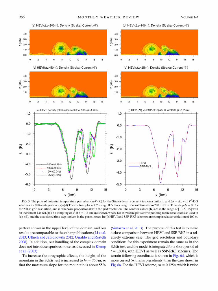
perature u0 (K) after 900 s for the Straka density current
is shown in Figs. 5a–d, with the grid spacings successively
halved from 200 to 25m. The time step is Dt5 0.16 s for
200-m grid resolution and decreases linearly with the
grid spacing. The results shown are with the P2 version
of the DG-NH model. This test was repeated with the
high-order (Pk, k 5 3, 4) spatial discretization with
a similar resolution, and the results were visually in-
distinguishable, showing an acceptable grid conver-
gence. It is observed that three Kelvin–Helmholtz rotors
develop as the grid resolution is refined. The numerical
results are comparable to other published results
(Ahmad and Linedman 2007; Norman et al. 2011; Li
et al. 2013), despite different contour values. This test
verifies the LDG second-order diffusion in an operator-
split configuration.
Figure 5e gives the horizontal profile of the potential
temperature perturbation u0 sampled along z5 1.2 km at
the same set of the grid resolutions as in Figs. 5a–d. The
three valleys in the right panel of Fig. 5e correspond to
the three Kelvin–Helmholtz rotors in Figs. 5a–d. As the
resolution goes higher, more fine features of the current
are captured reflecting the multiscale nature of the flow.
Our results agree well with the multimoment FV
method (Li et al. 2013) and high-order DG method
(Giraldo and Restelli 2008). To compare the perfor-
mance of HEVI and SSP-RK3, the profile of potential
temperature perturbation along z 5 1.2 km for Dz 5100m is shown in Fig. 5f. The result of theHEVI scheme
is visually in line with that of SSP-RK3, which demon-
strates the robustness of the HEVI-DG combined with
the LDG diffusion.
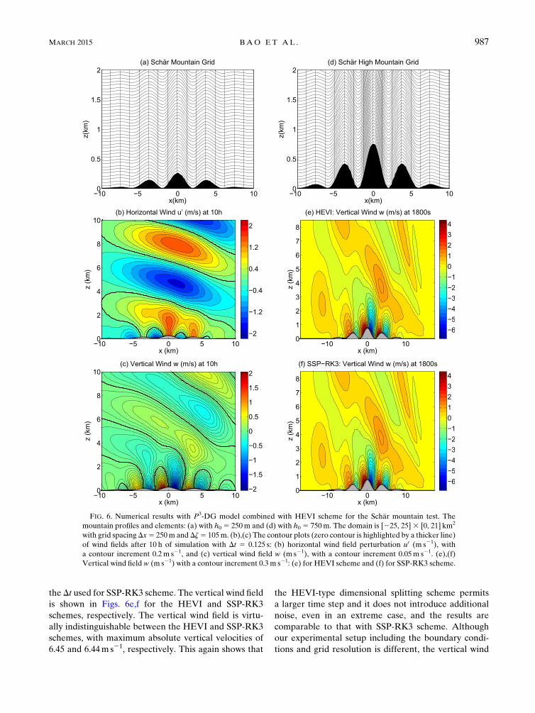
4) SCHÄR MOUNTAIN TEST
We consider the Schär mountain test (Schär et al.2002) to evaluate the performance of our HEVI scheme
in handling complex topography. The Schär mountaintest simulates the generation of gravity waves by a con-stant horizontal flow field in a uniform stratified atmo-sphere impinging on a nonuniform mountain range. Theprofile of the mountain range is given as
h(x)5 h0 exp
2x2
a20
!cos2
pxl
, (54)
where h0 5 250m, a0 5 5000m, and l 5 4000m. The
terrain-following, height-based coordinate in (4) takes
effect in this test case and is shown in Fig. 6a. The gravity
waves are composed of two major spectral components:
the large-scale hydrostatic waves propagate deeply in
the vertical, while the small-scale nonhydrostatic waves
decay rapidly as the altitude increases.
The initial state of the atmosphere has a constant
horizontal flow of u0 5 10ms21 and the Brunt–Väisäläfrequency is Nf 5 0.01 s21. The reference potential
temperature u can be computed from (47) using u0 5280K. The simulation is carried out in the domain of
[225, 25]3 [0, 21] km2. No-flux boundary conditions are
imposed at the bottom boundary and nonreflecting
boundary conditions are used along the top, left, and
right boundaries. The sponge layers are placed in the
region of z$ 9 km with ttop 5 0.28 for the top boundary
and jxj $ 15 km with tlat 5 0.18 for the lateral outflow
boundaries. Here P3-DG is used and the grid resolution
is chosen asDx5 250mandDz5 105m (Nx5 50,Nz5 50),
which leads to Dx/Dz ’ 2. We used a different aspect
ratio than the one used in Li et al. (2013), Ullrich and
Jablonowski (2012), and Giraldo and Restelli (2008),
where Dx/Dz ’ 1, because this makes HEVI scheme
more challenging. The simulation time is tT 5 10h
(36 000 s) with Dt 5 0.125 s for the HEVI scheme and
Dt5 0.065 s for the SSP-RK3 scheme. Figures 6b and 6c
show the contours of the horizontal and vertical wind
fields at 10 h in the region [210, 10] 3 [0, 10] km2 for
visualization. No visually distinguishable difference is
observed between the results of SSP-RK3 scheme and
HEVI scheme. There is no unphysical distorted wave
MARCH 2015 BAO ET AL . 985
pattern shown in the upper level of the domain, and our
results are comparable to the other publications (Li et al.
2013; Ullrich and Jablonowski 2012; Giraldo and Restelli
2008). In addition, our handling of the complex domain
does not introduce spurious noise, as discussed in Klemp
et al. (2003).
To increase the orographic effects, the height of the
mountain in the Schär test is increased to h0 5 750m, so
that the maximum slope for the mountain is about 55%
(Simarro et al. 2013). The purpose of this test is to make
a close comparison between HEVI and SSP-RK3 in a rel-
atively extreme case. The grid resolution and boundary
conditions for this experiment remain the same as in the
Schär test, and themodel is integrated for a short period oft 5 1800 s, with HEVI as well as SSP-RK3 schemes. The
terrain-following coordinate is shown in Fig. 6d, which is
more curved (with sharp gradients) than the case shown in
Fig. 6a. For the HEVI scheme, Dt5 0.125 s, which is twice
FIG. 5. The plots of potential temperature perturbation u0 (K) for the Straka density current test on a uniform grid Dx5Dzwith P2-DG
schemes for 900-s integration. (a)–(d) The contour plots of u0 using HEVI in a range of resolutions from 200 to 25m. Time step Dt5 0.16 s
for 200-m grid resolution, and is otherwise proportional with the grid resolution. The contour values (K) are in the range of [29.5, 0.5] with
an increment 1.0. (e),(f) The sampling of u0 at z5 1.2 km are shown, where (e) shows the plots corresponding to the resolutions as used in
(a)–(d), and the associated time step is given in the parentheses. In (f) HEVI and SSP-RK3 schemes are compared at a resolution of 100m.
986 MONTHLY WEATHER REV IEW VOLUME 143
the Dt used for SSP-RK3 scheme. The vertical wind field
is shown in Figs. 6e,f for the HEVI and SSP-RK3
schemes, respectively. The vertical wind field is virtu-
ally indistinguishable between the HEVI and SSP-RK3
schemes, with maximum absolute vertical velocities of
6.45 and 6.44ms21, respectively. This again shows that
the HEVI-type dimensional splitting scheme permits
a larger time step and it does not introduce additional
noise, even in an extreme case, and the results are
comparable to that with SSP-RK3 scheme. Although
our experimental setup including the boundary condi-
tions and grid resolution is different, the vertical wind
FIG. 6. Numerical results with P3-DG model combined with HEVI scheme for the Schär mountain test. Themountain profiles and elements: (a) with h0 5 250m and (d) with h0 5 750m. The domain is [225, 25]3 [0, 21] km2
with grid spacingDx5 250m and Dz5 105m. (b),(c) The contour plots (zero contour is highlighted by a thicker line)
of wind fields after 10 h of simulation with Dt 5 0.125 s: (b) horizontal wind field perturbation u0 (m s21), with
a contour increment 0.2m s21, and (c) vertical wind field w (m s21), with a contour increment 0.05m s21. (e),(f)
Vertical wind field w (m s21) with a contour increment 0.3m s21: (e) for HEVI scheme and (f) for SSP-RK3 scheme.
MARCH 2015 BAO ET AL . 987
fields shown in Figs. 6e,f are similar to the corresponding
Fig. 3 of Simarro et al. (2013).
6. Summary and conclusions
We have proposed a moderate-order discontinuous
Galerkin nonhydrostatic (DG-NH) model based on the
compressible Euler equations in a 2D (x, z) Cartesian
plane, with a simple operator-splitting time integration
scheme. The model uses a terrain-following height-based
coordinate to handle the orography. For the atmospheric
simulation on the nonhydrostatic scale, a high aspect ratio
between the horizontal and vertical spatial discretiza-
tion imposes a stringent restriction on the explicit time
step size for the Euler system. To alleviate the dominant
effect due to large horizontal–vertical aspect ratio, the
so-called horizontally explicit and vertically implicit
(HEVI) scheme via the Strang splitting is proposed and
studied in ourDG-NHmodel. TheHEVI time-integration
scheme avoids the tiny time step limitations, inflicted by
the vertical grid spacing (Dz � Dx), and, therefore, theoverall CFL restriction on the time step is mainly de-
termined by the horizontal grid spacing (Dx).The accuracy of our HEVI DG-NH model is tested
under a suite of NH benchmark test cases. The numer-
ical results, which are in agreement with those in liter-
ature, show that the HEVI scheme is robust and capable
of relaxing the CFL constraint to the horizontal grid
spacing and yields accurate simulations, even though the
vertical grid spacing is greatly smaller than the hori-
zontal (Dx/Dz 5 10, 100). As expected, a second-order
temporal convergence is observed with the HEVI
scheme, and a third-order spatial convergence is obtained
with the HEVI scheme as well as the SSP-RK3 scheme,
which is consistent with the P2-DG discretization. We
have also implemented an LDG-type second-order dif-
fusion in a dimension-split manner to be consistent with
the HEVI formulation. The LDG diffusion effectively
eliminates the small-scale noise for the model and stabi-
lizes the flow field, as is shown in the Straka density
current test. Moreover, in the presence of orography
(Schär mountain test), no spurious wave pattern or noiseis detected from the results of our HEVI scheme, and thenumerical simulation is visually identical to that of theSSP-RK3 scheme.The HEVI scheme is a practical option and competi-
tive approach for global NH atmospheric modeling,
since the existing solver of the horizontal dynamics can
be greatly recycled as done in a typical split-explicit case
when implemented in a full 3D domain. Here we dem-
onstrate that it is a viable option for the high-order DG
method as well. However, the efficiency of the HEVI
scheme mainly depends on the performance of the 1D
implicit solver. Proper preconditioning is a possible
remedy for accelerating the Newton–Krylov Jacobian-
free solver, and work in this direction is progressing. Our
ultimate goal is to implement the HEVI-DG formula-
tion in the High-Order Method Modeling Environment
(HOMME) developed at NCAR, to extend it as a NH
framework. The attractive features of HOMME (ex-
cellent parallel efficiency) can be exploited for the re-
sulting NH dynamical core when HEVI-DG scheme is
implemented. Further investigation will be continued on
the application of the HEVI time-split scheme in the
HOMME framework.
Acknowledgments. The authors thank two anony-
mous reviewers for the insightful comments that
improved the manuscript, and Dr. Michael Toy for
a thorough internal review. The first author would like
to thank Prof. Henry M. Tufo for his support and en-
couragement. RDN would like to thank Dr. Seoleun
Shin and KIAPS, Seoul, South Korea, for their support.
This work was partially supported by the DOE BER
Program under Award DE-SC0006959.
APPENDIX
Diffusion
Consider the following scalar advection-diffusion
equation on an element Ve, with the known (constant)
diffusion coefficient n (m2 s21):
›U
›t1$ � F(U)5 n=2U . (A1)
We summarize the application of LDGdiffusion process
in the following steps. [In the following process the
subscript (�)h is dropped for simplicity.]
1) The key idea of the LDG approach is the introduc-
tion of a local auxiliary variable q 5 n$U, and
rewriting the above problem as a first-order system:
q2 n$U5 0, (A2)
›U
›t1$ � F(U)2$ � q5 0. (A3)
2) For the LDG method, Let the numerical fluxes U*,
q* in (A6) be evaluated in terms of jump [�] and
central f�g fluxes, defined as follows:
U*5 fUg1b � [U], q*5 fqg2b[q]2hk[U],
(A4)
fUg5 (U1 1U2)/2, [U]5 (U2 2U1)n;
fqg5 (q1 1 q2)/2, [q]5 (q22 q1) � n .
988 MONTHLY WEATHER REV IEW VOLUME 143
3) Discretize the above system in (A2) and (A3) using
the weak formulation (Green’s method). This is
done by first multiplying by a vector test function
F 2 Vd(V) (d is the dimension of the problem) in
(A2) and integrating by parts:ðVq �FdV5 n
�ð›V
U*F � n ds2
ðVU$ �FdV
�.
(A5)
4) The final weak formulation for the advection-
diffusion equation (A1) is obtained by using a test
function [u 2 V(V)], the Lax–Friedrichs flux F̂, and
combining (A5):
›
›t
ðVUu dV2
ðVF(U) � $u dV1
ð›V
F̂(U) � nu ds
1 n
ðVq � $u dV2 n
ð›V
q* � nu ds5 0.
(A6)
5) In practice this is done in two stages. First, evaluate q
in (A5) using the above fluxes and then evaluate (A6).
Note that various second-order diffusions can be
formulated by carefully choosing the parameter valuesb
and hk, which are BR2, Bauman–Oden, and ‘‘flip-flop,’’
etc. [see Cockburn and Shu (1998) for multiple variants
of theLDGmethod]. The constantsb5 n/2 andhk5 0 are
set for most test cases considered herein, nevertheless,
other options are available in the DG-NH model.
REFERENCES
Ahmad, N., and J. Linedman, 2007: Euler solutions using flux-
based wave decomposition. Int. J. Numer. Methods Fluids, 54,
47–72, doi:10.1002/fld.1392.
Alexander, R., 1977: Diagonally implicit Runge–Kutta methods
for stiff O.D.E.’s. SIAM J. Numer. Anal., 14, 1006–1021,
doi:10.1137/0714068.
Ascher, U. M., S. J. Ruuth, and R. J. Spiteri, 1997: Implicit-explicit
Runge–Kutta methods for time-dependent partial differential