Hot-air optical turbulence generator for the testing ofadaptive optics systems: principles and characterization
Onur Keskin, Laurent Jolissaint, and Colin Bradley
A statistically repeatable, hot-air optical turbulence generator, based on the forced mixing of two air flowswith different temperatures, is described. Characterization results show that it is possible to generate anyturbulence strength up to CN
2 �h � 6 � 10�10m1�3, allowing a ratio of beam diameter to Fried’s parameteras large as D�r0 � 25 for one crossing through the turbulator or D�r0 � 38 for two crossings. The outerscale �L0 � 133 � 60 mm� is found to be compatible with the turbulator mixing chamber size �170 mm�,and the inner scale �l0 � 7.6 � 3.8 mm� is compatible with the values in the literature for the freeatmosphere. The temporal power spectrum analysis of the centroid of the focused image shows goodagreement with Kolmogorov’s theory. Therefore the device can be used with confidence to emulaterealistic turbulence in a controlled manner. A calibrated CN
2 profile, both in layer altitude and strength,is necessary for the testing of off-axis adaptive optics correction (multiconjugate adaptive optics). Testingwas done to calibrate the CN
This paper describes a simple, characterized, andstatistically repeatable optical turbulence generatorbased on the forced mixing of cold and hot air for usein laboratory testing of adaptive optics (AO) systems.It is an alternative to other techniques to simulatethe optical effect of atmospheric turbulence, such asetched rotating phase screens that are expensive tomanufacture and do not allow turbulence strengthadjustment. This limitation prevents real-time as-sessment of AO control system performance versusturbulence strength and particularly high-� events(e.g., sudden bursts of turbulence). The AdaptiveOptics Laboratory at the University of Victoria iscurrently investigating multiconjugate adaptive op-tics (MCAO) and multiobject adaptive optics (MOAO)systems. Therefore, a hot-air optical turbulence gen-
erator, based on a previous design1 (the prototype),has been developed.
To generate real optical turbulence (i.e., turbulentfluctuation of the refractive index), one needs to cre-ate dynamic turbulence (i.e., velocity) and tempera-ture fluctuation of the airflow. This is achieved bymixing two airflows with different temperatures in aconfined space: the turbulence chamber. The air in-take at one end of the channel remains at room tem-perature (cold intake), the other intake is heated (hotintake), and both fans are operated at identical fixedvelocities. The turbulence generator is versatile foremulating CN
2 and wind velocity by changing the fanspeeds and �T. Because the prototype was made outof wood, temperature differences were limited to ap-proximately 40 K, giving rise to r0 values of a mini-mum of �4 mm. To create stronger turbulence (i.e.,smaller r0), an all-aluminum design was developedallowing a maximum hot intake temperature of�200 °C.
In the MCAO and MOAO studies, anisoplanatismis a critical issue, and for that reason it is necessaryto reproduce off-axis decorrelation of the opticalturbulence in the laboratory environment. For theexperiments at the University of Victoria AO bench,it has been computed that the reproduction of aniso-planatism effects can be achieved by emulating twolayers of turbulence with equivalent thickness of
O. Keskin ([email protected]) and C. Bradley are with theDepartment of Mechanical Engineering, University of Victoria,P.O. Box 3055, Station CSC, Victoria, British Columbia V8W 3P6,Canada. L. Jolissaint is with the Herzberg Institute of Astro-physics, National Research Council, Victoria, British Columbia,Canada, and Fonds National de la Recherche Scientifique, Berne,Suisse.
Received 24 August 2005; revised 16 January 2006; accepted 23February 2006; posted 22 March 2006 (Doc. ID 64397).
�1 km. This is larger than the natural case (�100 m)but acceptable to demonstrate deformable mirrorconjugation. These layers are positioned at equiva-lent altitudes of 5 and 15 km relative to the AO sys-tem’s entrance pupil.
The Fried parameter �r0� of the turbulator has beencalibrated versus the temperature difference ��T �.The CN
2 profile can be simulated using either twoturbulence generators in series or two optical beampasses through one turbulator. The former approachprovides layer independence, whereas the latter re-quires no beam overlap to avoid spatiotemporal cor-relation between the two layers. The multipassscheme also requires altering the beam diameter toachieve a variable D�r0 per layer.
The slope detection and ranging (SLODAR) tech-nique2 was performed to characterize the CN
2 profile.The results of characterizing a turbulent layer arepresented. In Section 2 we review the effect of at-mospheric turbulence on optical beam propagation.Section 3 outlines the turbulator design. Section 4discusses the principles and experiments of charac-terization methods, and discussions and conclusionsare presented in Sections 5 and 6, respectively.
2. Effect of Atmospheric Turbulence
A. Dynamic Turbulence
Dynamic turbulence, i.e., turbulence of the air veloc-ity field, arises when the fluctuations of the velocityenergy rate ��U 2� are much larger than the energythat can be dissipated by viscous friction:
Re �kinetic energy
dissipated energy �UL�
�� 1, (1)
where Re is the Reynolds number, L is the flow scale,and � is the kinematic viscosity 15 � 10�6�m2�s�. Inthe free atmosphere, Re is generally in the range of106–1010 and it can be assumed that the free atmo-sphere is fully turbulent under most conditions.
Kolmogorov’s theory of atmospheric turbulence de-scribes the spatiotemporal properties of the turbu-lence.3 The idea is that the turbulent flow is limitedby an outer spatial scale, whereas the kinetic energyfluctuation is injected by a large-scale displacementforcing of the wind. From this scale, after the formingof the turbulent eddies, the air flow breaks down tosmaller and smaller eddies up to an inner spatialscale where the kinetic energy is dissipated due to theviscous friction (the energy cascade of the turbulentflow).
B. Optical Turbulence and Fried’s Parameter
On the basis of the fundamental Kolmogorov hypoth-esis, stating that the energy flow rate is constant fromlarger to smaller eddies,4,5 we show that in homoge-neous and isotropic turbulence the structure functionof the temperature field is defined by
DT��h� � ��T�rh� �h� � T�rh��2r, (2)
which becomes
DT��h� � DT��h� � CT2�2�3, (3)
where CT2 defines the structure constant of the tem-
perature field. Equation (3) is the starting point forthe development of the theory of optical effects of theatmospheric turbulence.
The mixing of air masses at different densities, dueto dynamic turbulence, creates a random and turbu-lent field of refractive index. The refractive index fluc-tuation is directly proportional to the air density asgiven by the Dale–Gladstone law: n � 1 � nP�T,where n � 80 � 10�8 K�Pa, P is the air pressure, andT is the air temperature. If the temperature field isturbulent, so will be the refractive index, and itsstructure function is given by
DN��� � CN2�2�3, (4)
where CN2 defines the structure constant of the re-
fractive index, linked to CT2 by
CN2 � nP
T 2 �2
CT2, (5)
and, because it can be shown that CT2 � �T 2, it be-
comes3
CN2 �nP
T 2 �2
��T�2, (6)
where �T 2 is the temperature fluctuation variancewithin the turbulent flow (see also Lukin andSazanovich6 for a measurement of the CT
2 and CN2
relationship). Equation (5) is used as the fundamen-tal relation of the hot-air turbulence generator.
The Fried7 parameter �r0� is defined as the diame-ter of the telescope having the same Strehl resolution(integral of the optical transfer function) as the at-mospheric optical transfer function. It can also beseen as a measure of the coherence length of theaberrated optical phase. The parameter is wave-length dependent and related to the refractive indexstructure constant8 by
r0�5�3 � 0.4234�2�� �2 �
0
�
CN2�h�dh, (7)
where � is the optical beam wavelength.The main effect of the optical turbulence in an
optical beam having a diameter D is to create phaseaberrations. When expressed in the Zernike polyno-mial basis, the aberration variances can be shown tobe proportional to the ratio �D�r0�5�3 and decreasewith the aberration’s radial order n.9
Optical turbulence is created in the laboratory bymixing hot and cold air with a judicious selection oftemperature difference, wind velocity (fan power),and optical beam diameter to achieve D�r0 ratioscompatible with the average working conditions atgood astronomical sites. The turbulence generatorhas one layer, and it will be assumed that CN
2 re-mains constant in this layer. In Eq. (7) the integralcan be replaced by the factor CN
2�h, where �h is thelayer thickness. Note that r0 is temperature depen-dant via the CN
2 temperature dependence. This char-acteristic enables its value to be tuned by changingthe temperature difference between the hot and coldintakes.
C. Outer- and Inner-Scale Effects of the OpticalTurbulence
The outer scale L0 is the upper limit of the turbulentflow extension. This scale limit has the effect of damp-ing the low-order optical aberrations, relative to thecase of an infinite extension of the flow10 as assumedin the Kolmogorov11 model; therefore the Kolmogorovmodel overestimates the effect of turbulence. The VonKarman12 (VK) empirical phase power spectrum isgenerally used to take into account the effect of L0damping on the low orders (i.e., low spatial frequen-cies) and is given by
��f � �0.023
r05�3 f 2 �
1
L02��11�6
, (8)
where f is the spatial frequency in the pupil plane.The inner scale l0 has basically the same effect for
the high-order aberrations, and the l0 damping factorof the phase power spectrum can be approximatedwith
��l0� � exp��l02f 2�. (9)
Another more sophisticated model for inner-scaledamping is provided by the Hill–Andrews empiricaldamping factor13 but is not discussed here. Thecutting spatial frequency associated with a givenZernike polynomial in the radial order n is given by14
fc � 0.37�n � 1��D. Replacing the spatial frequency inEq. (9) with fc, the inner-scale damping becomes
��l0� � exp��0.137�n � 1�2�l0�D2��, (10)
which gives an empirical relation that can be used toassess the D�l0 ratio from a Zernike aberration vari-ance experimental measurement.
Because of the strong decrease of the VK powerspectrum at high frequencies, the l0 damping effectis generally negligible for astronomical telescopes,where D �� l0. For our turbulator, however, the effectof l0 must be taken into account: l0 damping is notice-able if D is greater than �l0.
D. Temporal Properties of the Optical Turbulence
The temporal power spectrum of the Zernike aberra-tions induced by the turbulence has a power-law de-pendency in f 0 or f �2�3 at low frequencies and �f �17�3
at high frequencies.13 The temporal cutting fre-quency, or knee frequency, fc between these two re-gimes for a radial order n is given by
fc � 0.3�n � 1�VD, (11)
where V is the main layer velocity, n is the radialorder of the polynomial, and D is the diameter of thetelescope. To reproduce the same dynamical behaviorin the turbulator, it is in principle sufficient to repro-duce the V�D ratio.
Equation (11) assumes a single layer, frozen(Taylor hypothesis) to the beam of the telescope. Inour turbulator, due to its structure, the Taylor hy-pothesis does not apply, but we will see (Section 4)that this is in fact a minor problem.
3. Turbulence Generator Design
A. Design Specifications for the Turbulence Generator
In Section 2, spatiotemporal properties of the turbu-lent phase aberrations were defined by ratios. Toemulate the same properties, as measured on theastronomical observation sites, the following ratiosmust be reproduced in the turbulator: D�r0, D�L0,and D�l0, which are related to the spatial properties,and D�V, which is related to the temporal properties.
For a telescope of 8 m in diameter, in the free at-mosphere, typical values can be given as D�r0 � 40,D�L0 � 0.08 → 0.8, D�l0 � 600 → 2000, and D�V �0.4 → 1.6 s. If a 42 mm diameter optical beamis sent through the turbulator, r0 � 1 mm canbe achieved by reproducing the ratio ranges withL0 � 525–52 mm, l0 � 0.02–0.07 mm, and V �0.026–0.1 m�s. Unfortunately, the inner scale is notadjustable in the turbulator because real atmosphereis being used, so l0 will be in the usual range of a fewmillimeters. Note that the lack of inner-scale adjust-ability is not a drawback because the high-order ab-errations are not intended to be corrected. Indeed,with a beam diameter of 42 mm and an l0 value of�6 mm, we find [approximation (10)] that the l0damping becomes significant �1�e� for radial ordersabove 18 (i.e., Zernike aberrations J � 172 andabove). For a moderate order AO system like MCAOor MOAO this attenuation is not an issue as aberra-tion amplitude is needed mostly at low orders, andhigh-order aberrations are in principle not affected bythe correction, so it would still be possible to evaluatethe performance of the AO system by looking at thelow-order aberration attenuation. The isoplanatic an-gle of a turbulent profile is given by15
where �h is the average altitude of the turbulentlayers, relative to the telescope entrance pupil andweighted by the layer’s strength.
If the isoplanatic angle must also be reproduced,the CN
2 thickness must be broadened at the turbula-tor level, which can be done by adding several turbu-lators in series. Unfortunately, this solution is notpractical due to the limited space on most AObenches. Using the same turbulator several times(not yet implemented) is an alternative that can beachieved by folding the optical beam back and forththrough the same turbulent area and carefully avoid-ing beam overlap (folding of the beam was previouslystudied by Smith and co-workers16,17). The beam di-ameter would have to be expanded or shrunk if onewanted to generate different D�r0 values. Unwantedspatiotemporal cross correlation between the emu-lated layers can be minimized by a careful separationof the beams into the turbulent chamber.
To put things in perspective, if the turbulator is setat an r0 of 2 mm, with a double pass, then an averageturbulent layer distance (equivalent altitude) of 13 mwill give an isoplanatic patch of �10 arc sec, which is
a typical value for most observatories. Such a dis-tance, while not small, is certainly manageable in theconstrained space of an AO laboratory, using a set ofnearly parallel mirrors to fold the optical beam sev-eral times before resending it through the turbulator.
B. Design Considerations
Our turbulence generator (illustrated in Fig. 1) ismade of aluminum and has plates that divide theinner area into two ducts so that hot- and cold-airintake can mix in the turbulent chamber.
Variable fan speeds were selected. Off-the-shelfheaters, which fit the turbulator’s dimensions, wereused to allow maximum temperature differences of�200 K. Honeycombs regularized the air flow beforethe mixing chamber.
Because the temperature is a critical parameter, atemperature mapping on the hot- and cold-air side ofthe turbulence generator was required. Indeed thedissipation of the hot air into the duct could reducethe optical turbulence strength in the generator. Themapping proved that the optical beam path crossedthe turbulent area where the temperature differencewas maximum, optimizing the disturbance effect onthe laser beam.
C. Optical Setup for Turbulator Characterization
The experimental arrangement is shown in Fig. 2.The key features of this arrangement are the follow-ing:
Y A collimated laser beam is created from a pointlight source (a laser through a spatial filter in ourexperiment).
Y Neutral filters are used to prevent saturationor damage to the CCD chip.
Y A stop is placed after the turbulence generatorhaving the role of the entrance pupil on a telescope.
Y The last lens has the function of simulating thetelescope optics as seen from the CCD camera.
Y The long-exposure focused images of the turbu-lent beam are collected by the CCD camera for thefull width at half-maximum (FWHM) experiment(Subsection 4.A). For the angle-of-arrival (AoA) ex-periment (Subsection 4.B), the displacement of theinstantaneous image is tracked by the CCD camerawith a 522 frames�s sampling frequency.
Fig. 1. Turbulence generator.
Fig. 2. Optical setup for the Fried parameter characterization.
SLODAR setup was implemented. The requiredsetup is similar to the one shown in Fig. 2. The sameturbulence generator is used. A Shack–Hartmann(SH) lenslet array is placed in a plane conjugated tothe entrance pupil. However, for the experiment twoor more guide stars (GS) had to be simulated with aknown angle of separation between them. For thatpurpose, a pigtailed laser diode unit, with fibersseparated by a known angle (1.7 arc sec as seen fromthe entrance pupil), was used. To obtain the knownangle of separation in the experimental setup, a lasermount unit was manufactured by Micro-Electro-Discharge Machining to obtain a precise 30 �m sep-aration between the two star images on the SHwavefront sensor (WFS) focal plane, corresponding toa separation of two pixels on the CCD. The diverg-ing light from the fibers is collimated to a 25 mmdiameter.
4. Principles and Experimentations of theCharacterization Methodologies
A. Full Width at Half-Maximum Experiment
The point-spread function (PSF) is the pattern pro-duced by the spread-out light from a single pointsource. The FWHM is the width of the light intensityprofile at half of the maximum peak intensity of thePSF. The maximum resolution available from a tele-scope of a diameter D is set by diffraction, in the idealcase of no turbulence, and the corresponding FWHMis �D where � is the wavelength. Optical turbulencebroadens the FWHM of long-exposure images, and toa first approximation the contribution of the telescopeand atmosphere on the FWHM add in quadrature. Inthe Kolmogorov regime, we get
FWHM ��FWHMtelescope�2 � �FWHMatmosphere�2
�D�1 � �D�r0�2. (13)
When L0 � �, the FWHMatmosphere � 0.98 �D, so Eq.(13) becomes an upper limit; this equation then pro-vides a fast and simple way of determining an upperlimit for r0.
The long-exposure turbulent PSF is shown inFig. 3. Seeing-limited FWHM values gathered with�T � 53 K and �T � 0 K (no turbulence) are com-pared to assess the increase of the FWHM. Fromthese values [using Eq. (13)] we found a Fried param-eter (at 500 nm) of r0 � 7.0 � 0.8 mm.
In this experiment, the damping effect due to theinfinite outer- and inner-scale turbulence is not takeninto account. Therefore, the actual r0 can certainly beexpected to be smaller than 7.0 mm.
B. Angle-of-Arrival Method
1. DescriptionThe AoA is defined as the mean slope of the turbulentwavefront W�x, y� into the pupil P�x, y� of the tele-
scope, or the exit pupil of the turbulator in this ex-periment:
p �XC
FL�
��P�x, y��W�x �x, y�dxdy
��P�x, y�dxdy
, (14)
where FL is the focal length and XC is the x coordinateof the image centroid (see Fig. 2). Equation (14) isgiven for the x coordinate on the focal plane. Therelation for the y coordinate is the same as the xcoordinate and is instead obtained by derivation ver-sus y.
In the general case of a limited flow, the AoA vari-ance is given for a turbulent layer of thickness �h by18
�AoA2�x, y� � �2��4�30.033CN
2�h
���R2
fX,Y2�f 2 � L0
�2��11�6exp��l02 f 2�
� �2J1��Df ��Df �2
dfXdfY. (15)
Equation (15) has an analytic solution only in theinfinite scale regime �L0 � � and l0 � 0):
�AoA2�x, y� � 2.8375CN
2�hD�1�3
� 0.1698� �D�2�D�r0�5�3. (16)
We see that the AoA variance decreases when thepupil diameter is increased. In the limited regime,this is still the case, but with departure from the D�1�3
law at small and large values of D, due to the damp-ing effect of L0 and l0. Masciadri and Yernin18 havesuggested using this dependency as a way to measurethe L0 and l0 in turbulent flows. The characterizationof the turbulence generator using the AoA method isdone in two steps:
Y The heaters and the fans are set to a fixedtemperature difference and wind velocity. The dis-
Fig. 3. Left, PSF with turbulator off. Right, PSF with turbulatoron at �T � 53 K.
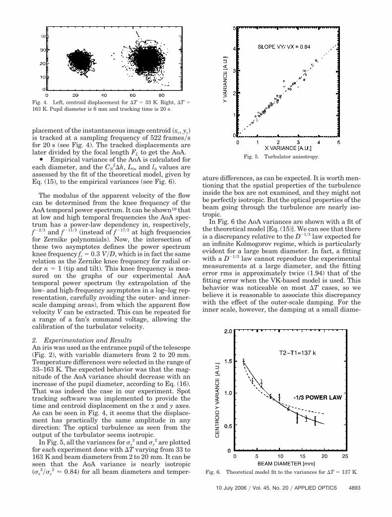
placement of the instantaneous image centroid �xc, yc�is tracked at a sampling frequency of 522 frames�sfor 20 s (see Fig. 4). The tracked displacements arelater divided by the focal length FL to get the AoA.
Y Empirical variance of the AoA is calculated foreach diameter, and the CN
2�h, L0, and l0 values areassessed by the fit of the theoretical model, given byEq. (15), to the empirical variances (see Fig. 6).
The modulus of the apparent velocity of the flowcan be determined from the knee frequency of theAoA temporal power spectrum. It can be shown19 thatat low and high temporal frequencies the AoA spec-trum has a power-law dependency in, respectively,f �2�3 and f �11�3 (instead of f �17�3 at high frequenciesfor Zernike polynomials). Now, the intersection ofthese two asymptotes defines the power spectrumknee frequency fc � 0.3 V�D, which is in fact the samerelation as the Zernike knee frequency for radial or-der n � 1 (tip and tilt). This knee frequency is mea-sured on the graphs of our experimental AoAtemporal power spectrum (by extrapolation of thelow- and high-frequency asymptotes in a log–log rep-resentation, carefully avoiding the outer- and inner-scale damping areas), from which the apparent flowvelocity V can be extracted. This can be repeated fora range of a fan’s command voltage, allowing thecalibration of the turbulator velocity.
2. Experimentation and ResultsAn iris was used as the entrance pupil of the telescope(Fig. 2), with variable diameters from 2 to 20 mm.Temperature differences were selected in the range of33–163 K. The expected behavior was that the mag-nitude of the AoA variance should decrease with anincrease of the pupil diameter, according to Eq. (16).That was indeed the case in our experiment. Spottracking software was implemented to provide thetime and centroid displacement on the x and y axes.As can be seen in Fig. 4, it seems that the displace-ment has practically the same amplitude in anydirection: The optical turbulence as seen from theoutput of the turbulator seems isotropic.
In Fig. 5, all the variances for �x2 and �y
2 are plottedfor each experiment done with �T varying from 33 to163 K and beam diameters from 2 to 20 mm. It can beseen that the AoA variance is nearly isotropic��x
2��y2 � 0.84� for all beam diameters and temper-
ature differences, as can be expected. It is worth men-tioning that the spatial properties of the turbulenceinside the box are not examined, and they might notbe perfectly isotropic. But the optical properties of thebeam going through the turbulence are nearly iso-tropic.
In Fig. 6 the AoA variances are shown with a fit ofthe theoretical model [Eq. (15)]. We can see that thereis a discrepancy relative to the D�1�3 law expected foran infinite Kolmogorov regime, which is particularlyevident for a large beam diameter. In fact, a fittingwith a D�1�3 law cannot reproduce the experimentalmeasurements at a large diameter, and the fittingerror rms is approximately twice (1.94) that of thefitting error when the VK-based model is used. Thisbehavior was noticeable on most �T cases, so webelieve it is reasonable to associate this discrepancywith the effect of the outer-scale damping. For theinner scale, however, the damping at a small diame-
Fig. 4. Left, centroid displacement for �T � 33 K. Right, �T �163 K. Pupil diameter is 6 mm and tracking time is 20 s.
Fig. 5. Turbulator anisotropy.
Fig. 6. Theoretical model fit to the variances for �T � 137 K.
ter is not really noticeable in Fig. 6, but because theinner-scale value extracted from the ensemble of ourmeasurement (given below) is definitely compatiblewith most other authors’ values, we believe that theinner-scale effect is present in our measurements andwould become more noticeable with a higher sam-pling of the AoA variance at low diameters—say inthe range of 1–5 mm.
Outer and inner scale. Because L0 and l0 are relatedonly to the dynamic properties of the turbulent flow,the outer and inner scales are not dependent on thetemperature differences occurring on the turbulence,and the mean values of L0 and l0 among all temper-ature difference measurements are L0 � 133 �60 mm and l0 � 7.6 � 3.8 mm. The L0 value is com-patible with the dimensions of the turbulence gener-ator’s mixing chamber �17 cm � 17 cm�, and the l0value is compatible with measurements made byother authors, e.g., Masciadri and Vernin18 �6 �1 mm� and Lukin and co-workers20,21 �2–6 mm�.
CN2�h and r. In Table 1 experimental values of
CN2�h and the Fried parameter r0 at 500 nm are
given. Using these r0 values and a beam diameter of42 mm, in the turbulence generator, it is possible toachieve D�R0 ratios as large as 25 for a single passand 38 for double passes. The difference of r0 valuesfrom the FWHM �r0 � 7.0 mm� and AoA experimentscan be explained by the damping effect of the outerand inner scales of the turbulence on the low- andhigh-order aberrations that were not taken into ac-count in the FWHM experiment.
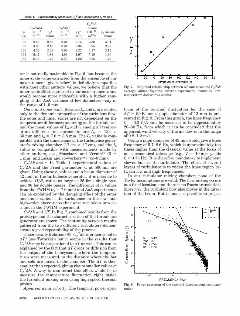
CN2�h and �T. In Fig. 7, combined results from the
prototype and the characterization of the turbulencegenerator are shown. The continuity between resultsgathered from the two different turbulators demon-strate a good repeatability of the process.
Theoretically [relation (6)], CN2�h is proportional to
�T 2 (see Tatarski3) but it seems in the results thatCN
2�h may be proportional to �T as well. This can beexplained by the fact that �T drops by diffusion fromthe output of the honeycomb, where the tempera-tures were measured, to the distance where the hotand cold are mixed in the chamber. The �T is thensmaller than expected, giving rise to smaller values ofCN
2�h. A way to counteract this effect would be tomeasure the temperature fluctuation right insidethe turbulent mixing area using high-speed thermalprobes.
Apparent wind velocity. The temporal power spec-
trum of the centroid fluctuation for the case of�T � 90 K and a pupil diameter of 12 mm is pre-sented in Fig. 8. From this graph, the knee frequencyfc � 0.3 V�D can be assessed to be approximately20–30 Hz, from which it can be concluded that theapparent wind velocity of the air flow is in the rangeof 0.8–1.2 m�s.
Using a pupil diameter of 42 mm would give a kneefrequency of 5.7–8.6 Hz, which is approximately tentimes higher than the classical value at the focus ofan astronomical telescope (e.g., V � 10 m�s yieldsfc � 0.75 Hz). It is therefore mandatory to implementslower fans in the turbulator. The effect of severallayers of turbulence is to widen the knee region be-tween low and high frequencies.
In our turbulator mixing chamber, none of theTaylor assumptions are valid: The flow mixing occursat a fixed location, and there is no frozen translation.Moreover, the turbulent flow also moves in the direc-tion of the beam. But it must be possible to project
Table 1. Experimentally Measured CN2 and Associated r0 Values
any movement of the air masses on an arbitrary num-ber of lateral frozen flow displacements (perpendicu-lar to the optical beam) with appropriate apparentvelocities. The fact that the temporal power spectrumof the AoA (Figs. 8 and 10) shows an asymptoticbehavior compatible with a Kolmogorov optical tur-bulence, a rather wide low- to high-frequency tran-sition range tends to support the assumption ofmultiple apparent layers with different velocities andCN
2. Indeed, as each layer has its own velocity andCN
2 intensity, each layer’s temporal power spectrumis displaced relative to each other. The result is thebroadening of the transition range between the �2�3and �11�3 parts of the total temporal power spec-trum.
C. Slope Detection and Ranging Method
The principle of the SLODAR technique is the follow-ing:
Y Two stars a few arcseconds apart are observedwith a slope WFS (SH, for instance).
Y The cross correlation of the time series of theslopes from lenslet to lenslet can be interpreted as ameasure of the CN
2 profile within the altitude rangewhere the two star beams overlap.
Practically, the cross correlation has to be decon-volved with the single-star autocorrelation (takenfrom any of the two stars), and the CN
2 is given by
CN2 � F�1�F�C��i, �j��
F�A��i, �j�����i, 0�, (17)
where F is the Fourier-transform operator, �i, j arethe lenslet cross-correlation shifts in the WFS focalplane, C��i, �j� are the cross correlation between thestars’ slopes (or centroid) time series �i, �j, and A isthe autocorrelation for the same shift.
CN2 is retrieved from the deconvolved cross-
correlation matrix along a line corresponding to theGS separation. In our case the two stars have beenoriented along the x axis of the WFS. To determinethe CN
2 profile absolute magnitude, we can use theturbulator’s calibration curve r0��T� built using theAoA experiment (see Fig. 7).
The vertical resolution of the CN2 measurement in
SLODAR mode is given by �H � D�ns��, where D isthe optical beam diameter, ns is the number of SHlenslets across the beam diameter (ten in our case),and is the angular separation of the two GSs, asseen from the entrance pupil of the SLODAR setup(45° in our case). The maximum sensing altitude isgiven by Hmax � D��.
The SLODAR experiment has been implementedfor temperature differences from 30 to 160 K, gener-ating r0 values from �3 to 1.7 mm as calculated fromAoA characterization. The centroid position for eachstar is tracked using an algorithm that is able to readseparately both regions on the CCD sublenslet im-ages around each star centroid. Ten thousand sam-ples are taken, with a frame rate of 522 Hz, short
enough to freeze the centroid motion during the ex-posure.
Figure 9 shows an example of centroid tracking forone of our measurements. Even with such a smallseparation (two pixels), the centroids for both starsare easily tracked. Mean values of the centroid timeseries are subtracted before computing the cross-correlation and autocorrelation matrices.
In Fig. 9 the centroid displacement of the two GSs,positioned at an angle of 45°, can be seen under theeffect of the turbulence. It is also clear that the dis-placement amplitude is practically the same for bothaxes and for both stars: The optical turbulence seemsisotropic.
Figure 10 shows the AoA temporal power spectrumfor both stars: the �2�3 and �11�3 power law ex-pected is clearly seen (dashed curves) for both stars.
Fig. 9. (Color online) Centroid movement for the two stars on asubimage lenslet.
Fig. 10. Centroid temporal power spectrum for both stars(�T � 90 K).
The knee frequency is �20 Hz, which gives, withD � 42 mm, an apparent velocity of 0.8 m�s.
With such a setup, ten repetitions of CN2 samples at
altitudes of 0 and 21.24 m are gathered. It turns outthat the (virtual) entrance pupil of the SLODARsetup is in the middle of the turbulator. Therefore, weexpected to find a one-layer CN
2 profile concentratedat the first �0 m� sample [approximation (17)].
Autocorrelation and cross-correlation algorithmshave been implemented, and the deconvolution wasdone using a maximum entropy algorithm. Figure 11shows an example of cross-correlation, autocorrela-tion, and deconvolved cross-correlation matrices. Aunique central peak is indeed seen in the deconvolvedCN
2 profile. The cross correlation is broader than theautocorrelation, which can be interpreted by the factthat the CN
2 profile is not a single thin layer. To seethe details of the CN
2 profile within the turbulator,the SLODAR resolution of the setup has to be in-creased to a few centimeters.
5. Discussion
In this section possible improvements in the setupare discussed. First, a SH WFS would be useful tocharacterize the turbulator’s high-order aberrations;measuring the damping effect of the inner scalewill be particularly interesting. The high-temporal-frequency measurements can also be performed moreprecisely using a SH WFS by the measurement ofeach mode’s temporal power spectrum. Second, a sen-sitive issue is the fan’s velocity: Clearly, the velocityin our turbulator is too high, and slower fans must beimplemented. The slower the air velocity, however,the more time the hot air has to cool before enteringthe mixing area, decreasing the optical turbulencestrength. Third, the vertical temperature gradientinto the turbulator can be decreased by turning theturbulator by 90° up around the axes of the inputpipes, so the air rising due to natural convection willsimply be embedded in the forced movement of theflow. The horizontal temperature gradient of the tur-bulator (the fact that �T 2 is not necessarily constantalong the horizontal path crossed by the light beam)can be improved by having double cold–hot half-channels instead of one. Fourth, the hot-air channelshould be thermally isolated up to the entrance of themixing area to get rid of heat loss and temperature
gradient within the channel, which might be a prob-lem when operating at low fan speeds, as statedabove. Fifth, we have implemented and tested onlythe SLODAR procedure here, but we have not doneany real CN
2 characterization. This said, on the basisof the fact that we were able to actually see a singlelayer at the apparent altitude we expected, with ourpoor vertical resolution, we have confidence that mul-tiple folding might work for implementing a CN
2 pro-file. Finally, the turbulator’s CN
2��T� calibrationcurve can be improved by increasing the number ofmeasurements and sampling in the �T range.
6. Conclusions
From the AoA experimentation, it can be concludedthat the spatiotemporal properties of the generatedturbulence are in good agreement with Kolmogorovand VK theories (including the effect of the outer andinner scales). Also, the generated optical turbulenceseems isotropic. The D�L0 and D�l0 values are withinthe expected range. L0 � 133 � 60 mm is compatiblewith the turbulator’s mixing chamber dimensions�170 mm � 170 mm�. If a higher L0 is required, thedimensions of the turbulence generator have to beincreased (or vice versa for a lower L0). D�r0 measure-ments are close to the specifications for an 8 m diam-eter telescope when a temperature difference of163 K is used. As the empirical relationship betweenCN
2 and �T is predictable (but can be made moreaccurate with a better sampling), it can be concludedthat higher-temperature differences will generatestronger optical turbulence. D�V is too small but isstill in the correction range of the MCAO controlsystem. A laboratory multiple-layer CN
2 profile thatcan be measured using the SLODAR technique, usinga hot-air turbulence generator, appears to be feasible.
The authors acknowledge the support of the Uni-versity of Victoria and the National Research Councilof Canada for their technical support and the FondsNational de la Recherche Scientifique Suisse. We alsothank the anonymous reviewers for their useful com-ments, leading to a significant improvement of thepaper.
Fig. 11. Case at �T � 160 K. Left, raw cross-correlation matrix. Center, autocorrelation matrix. Right, deconvolved cross-correlationmatrix.
References1. L. Jolissaint, “Optique adaptative au foyer d’un telescope de la
classe 1 metre,” (Université de Genève, Geneva, Switzerland,2000).
2. R. W. Wilson, “SLODAR: measuring optical turbulence alti-tude with a Shack-Hartmann wavefront sensor,” Mon. Not. R.Astron. Soc. 337, 103–108 (2002).
3. V. I. Tatarski, Wave Propagation in a Turbulent Medium(Dover, 1961).
4. A. M. Obukhov, “Structure of the temperature field in a tur-bulent flow,” Izv. Acad. Nauk. SSSR Ser. Geograf. Geofiz. 13,58 (1949) [German translation in Sammelband zur StatischenTheoric der Turbulenz (Akademie Verlag, 1958)].
5. A. M. Yaglom, “On the local structure of the temperaturefield in a turbulent flow,” Doklady Acad. Nauk. SSSR Ser.Geograf. Geofiz. 69, 73 (1949) [German translation in Sam-melband zur Statischen Theoric der Turbulenz (AkademieVerlag, 1958)].
6. V. P. Lukin and V. M. Sazanovich, “Investigations of turbulentcharacteristics in conditions of convection,” Atmos. OceanPhys. 14, 1212–1215 (1978).
7. D. L. Fried, “Optical resolution through a randomly inhomo-geneous medium for very long and very short exposures,” J.Opt. Soc. Am. 56, 1372–1379 (1966).
8. F. Roddier, “The effects of atmospheric turbulence in opticalastronomy,” in Progress in Optics, E. Wolf, ed. (North-Holland,1981), Vol. 19.
9. R. J. Noll, “Zernike polynomials and atmospheric turbulence,”J. Opt. Soc. Am. 66, 207–211 (1976).
10. D. M. Winker, “Effect of a finite outer scale on the Zernike
decomposition of atmospheric optical turbulence,” J. Opt. Soc.Am. A 8, 1568–1573 (1991).
11. A. N. Kolmogorov, “Local structure of turbulence in incom-pressible fluids with very high Reynold’s number,” Dokl. Akad.Nauk SSSR 30, 301–305 (1941).
12. T. Von Karman, “Progress in the statistical theory of turbu-lence,” J. Mar. Res. 7, 252–264 (1948).
13. A. Consortini and C. Innocenti, “Estimate of characteristicsscales of atmospheric turbulence by thin beams: comparisonbetween the Von Karman and Hill-Andrews models,” J. Mod.Opt. 51, 333–342 (2004).
14. J. M. Conan, G. Roussel, and P. Y. Madec, “Wave-front tem-poral spectra in high-resolution imaging through turbulence,”J. Opt. Soc. Am. A 12, 1559–1570 (1995).
15. D. L. Fried, “Anisoplanatism in adaptive optics,” J. Opt. Soc.Am. 72, 52–61 (1982).
16. J. Smith, T. H. Pries, K. J. Shipka, and M. A. Hamiter, “High-frequency plane-wave filter function for a folded path,” J. Opt.Soc. Am. 62, 1183–1187 (1972).
17. J. Smith, “Folded-path weighting function for a high-frequencyspherical wave,” J. Opt. Soc. Am. 63, 1095–1097 (1973).
18. E. Masciadri and J. Vernin, “Optical technique for inner-scalemeasurement: possible astronomical applications,” Appl. Opt.36, 1320–1327 (1997).
19. G. A. Tyler, “Bandwidth considerations for tracking throughturbulence,” J. Opt. Soc. Am. A 11, 358–367 (1994).
20. V. P. Lukin and V. V. Pokasov, “Optical wave phase fluctua-tions,” Appl. Opt. 20, 121–135 (1981).
21. V. P. Lukin and V. L. Mironov, “Phase measurements of innerscale of atmospheric turbulence,” Atmos. Ocean Phys. 12,1317–1319 (1976).