Household Intertemporal Behavior: a Collective - UCLA Economics

Household Intertemporal Behavior: a Collective Characterization

and a Test of Commitment∗

Maurizio Mazzocco†

UCLA and University of Wisconsin-Madison

March 2006

Abstract

In this paper, a formal test of intra-household commitment is derived and performed. To

that end, two models of household intertemporal behavior are developed. In both models, house-

hold members are characterized by individual preferences. In the first formulation, household

decisions are always on the ex-ante Pareto frontier. In the second model, the assumption of

intra-household commitment required by ex-ante efficiency is relaxed. It is shown that the full-

efficiency household Euler equations are nested in the no-commitment Euler equations. Using

this result, the hypothesis that household members can commit to future allocations of resources

is tested using the Consumer Expenditure Survey. I strongly reject this hypothesis. It is also

shown that the standard unitary framework is a special case of the full-efficiency model. How-

ever, if household members are not able to commit, household intertemporal behavior cannot

be characterized using the standard life-cycle model. These findings have two main implica-

tions. First, policy makers can change household behavior by modifying the decision power of

individual household members. Second, to evaluate programs designed to improve the welfare

of household members, it would be beneficial to replace the standard unitary model with a

characterization of household behavior that allows for lack of commitment.

∗An earlier version of this paper was circulated under the title: “Household Intertemporal Behavior: a Collective

Characterization and Empirical Tests”. I am very grateful to the editor, Maitreesh Ghatak, two anonymous referees,

Orazio Attanasio, Pierre-Andre Chiappori, James Heckman, John Kennan, Annamaria Lusardi, Costas Meghir, and

Bernard Salanie, for their insight and suggestions. For helpful comments, I would also like to thank the participants

at the 27th Seminar of the European Group of Risk and Insurance Economists, at the AEA Meetings, at the

Southeast Economic Theory and International Economics Meetings and at seminars at New York University, Ohio

State University, University College of London, University of California at Irvine, University of Chicago, University of

Pennsylvania, University of Quebec at Montreal, University of Wisconsin-Madison, and Western Ontario University.

Errors are mine.†Maurizio Mazzocco, Bunche Hall, Los Angeles, CA 90095. Email: [email protected].

1

1 Introduction

The theoretical and empirical literature on household intertemporal decisions has traditionally

assumed that households behave as single agents. One of the main drawbacks of this approach

is that the effect of intra-household commitment on intertemporal decisions cannot be analyzed

and tested. The main goal of this paper is to test whether household members can commit to

future allocations of resources and to examine the implications of the outcome of the test for policy

analysis. To that end, the household is modeled as a group of agents making joint decisions.

A good understanding of intra-household commitment is important to determine the potential

effects of social programs which attempt to raise the welfare of poor families by modifying household

decisions. Too see this consider Progresa, a Mexican program that provides cash transfers to female

heads of poor rural households on condition that the children attend school and that the family

visits selected health centers regularly. This program has two components. The first component

is an attempt to change the budget constraint of the household, and therefore its decisions, by

allocating resources that are conditional on a particular type of household behavior. The effect

of this component has been widely studied and it is generally well understood. The objective of

the second component is to change the decision power of individual household members, and hence

household behavior, by allocating financial transfers to the female head of the household. The effect

of the second component depends on the degree of commitment characterizing the household, which

cannot be evaluated under the assumption that households behave as single agents. This paper is

one of the first attempts to determine under which conditions household decisions can be modified

by changing the individual decision power and to test these conditions.

Specifically, this paper makes three contributions to the literature on household intertemporal

behavior. First, two models are developed to characterize the intertemporal behavior of the house-

hold and the effect of social programs on its decisions. In both frameworks, household members

are characterized by individual preferences. In the first model, household decisions are efficient

in the sense that they are always on the ex-ante Pareto frontier. Ex-ante efficiency requires the

household members to be able to commit to future allocations of resources. In the second model,

the assumption of intra-household commitment is relaxed.

The two models clarify the importance of understanding intra-household commitment in de-

signing a social program. If family members can commit formally or informally to future plans,

only the individual decision power at the time of household formation affects household decisions.

Consequently, any social program designed to change household behavior by modifying the indi-

vidual decision power will generally fail. By contrast, in the absence of commitment, household

decisions depend on the decision power in each period. This implies that a social program that

changes the wife’s and husband’s decision power will modify household decisions and the welfare

2

of family members.

As a second contribution, a formal test of commitment is derived and implemented. It is shown

that the full-efficiency household Euler equations are nested in the no-commitment household Euler

equations. To provide the intuition behind this result, let a distribution factor be one of the variables

affecting the individual decision power. Under ex-ante efficiency, only the individual decision power

at the time of household formation can influence household decisions. As a consequence, the only

set of distribution factors relevant to explain household behavior is the set containing the variables

known or predicted at the time the household was formed. It is shown that this has a main

implication for household Euler equations: the distribution factors should enter the household

Euler equations only interacted with consumption growth. If the assumption of commitment is

relaxed, the individual decision power in each period can influence the behavior of the household.

Consequently, its decisions can be affected by the realization of the distribution factors in each

period. This implies that the distribution factors should enter the household Euler equations not

only interacted with consumption growth, but also directly and interacted with future consumption.

Based on this result, intra-household commitment can be tested using a panel containing infor-

mation on consumption. In this paper, the test is implemented using the Consumer Expenditure

Survey (CEX) and the hypothesis of intra-household commitment is strongly rejected. This finding

indicates not only that commitment is violated, but also that the individual decision power varies

frequently enough after household formation to enable the test to detect the effect of these changes

on consumption dynamics. The main implication of this finding is that policies that affect the

intra-household balance of power will generally modify the welfare of household members. Social

programs like Progresa, policy recommendations designed to modify the marriage penalty, and

labor policies proposing differential tax treatments for the primary and secondary earners are only

a subset of such policies.

As an additional contribution, it is shown that the standard unitary model, in which a unique

utility function is assigned to the entire household, is a special case of the full-efficiency model. How-

ever, if the assumption of commitment is not satisfied, household intertemporal behavior cannot be

represented using the unitary model. This result, jointly with the outcome of the commitment test,

suggests that it would be beneficial to replace the unitary model with a collective characterization

of household decisions to evaluate social programs designed to modify the intertemporal behavior

of the household.

To derive the test of intra-household commitment, this paper extends the static collective model

introduced by Chiappori (1988, 1992) to a dynamic framework with and without commitment. The

static collective model has been extensively studied, tested, and estimated. Manser and Brown

(1980) and McElroy and Horney (1981) are the first two papers that characterize the household as

a group of agents making joint decisions. In those papers the household decision process is modeled

3

using a Nash bargaining solution. Apps and Rees (1988) and Chiappori (1988; 1992) generalize the

proposed model to allow for any type of efficient decision process. Thomas (1990) is one of the first

papers to test the static unitary model against the static collective model. Browning, Bourguignon,

Chiappori, and Lechene (1994) perform a similar test and estimate the intra-household allocation of

resources. Blundell, Chiappori, Magnac, and Meghir (2001) develop and estimate a static collective

labor supply framework that allows for censoring and nonparticipation in employment.

The present paper contributes to a new literature which attempts to model and test the intertem-

poral aspects of household decisions using a dynamic collective formulation. Basu (forthcoming)

discusses a model of household behavior under no-commitment using a game-theoretic approach.

Ligon (2002) proposes a no-commitment model of the household that has the same features as the

one analyzed in this paper. Lundberg, Startz, and Stillman (2003) use a collective model without

commitment to explain the consumption-retirement puzzle. Mazzocco (2004) studies the effect

of risk sharing on household decisions employing a full-efficiency model. Duflo and Udry (2004)

test whether household decisions are Pareto efficient using data from Cote D’Ivore. Aura (2004)

discusses the impact of different divorce laws on consumption and saving choices of married couples

that cannot commit. Lich-Tyler (2004) employs a repeated static collective model, a model with

commitment, and a model without commitment to determine the fraction of households in the

Panel Study of Income Dynamics (PSID) which make decisions according to the three different

models.

This paper is related to the empirical literature on Euler equations in two ways.1 First, the test

of intra-household commitment is derived using household Euler equations. Second, the outcome

of the commitment test provides an alternative explanation for the rejection of the household Euler

equations obtained using the unitary model. A well-known result in the consumption literature

is that household Euler equations display excess sensitivity to income shocks. The two main

explanations are the existence of borrowing constraints and non-separability between consumption

and leisure.2 The evidence described in this paper indicates that cross-sectional and longitudinal

variation in relative decision power explain a significant part of the excess sensitivity of consumption

growth to income shocks.

Social programs with the features of Progresa have been widely evaluated in the past five

years. Behrman, Segupta, and Todd (2001), Attanasio, Meghir, and Santiago (2001), and Todd

and Wolpin (2003) are only a few of the papers in this literature. This paper contributes to this line

of research in two respects. First, it clarifies the conditions under which policy makers can affect

household decisions by modifying its members’ decision power. Second, it provides and performs a1 See Browning and Lusardi (1996) for a comprehensive survey of this literature.2 See for instance Zeldes (1989) and Runkle (1991) for the first explanation and Attanasio and Weber (1995) and

Meghir and Weber (1996) for the second one.

4

test which indicates that these conditions are satisfied in U.S. data.

The paper is organized as follows. In section 2 the full-efficiency and no-commitment collective

models are introduced. Section 3 analyzes the conditions under which the standard life-cycle model

is equivalent to the collective formulation. In section 4 a test of intra-household commitment is

derived. Section 5 discusses the implementation of the test and section 6 presents the data used in

this paper. Section 7 examines some econometric issues and section 8 reports the results. Section

9 simulates the no-commitment model and tests commitment using the simulated data. Some

concluding remarks are presented in the final section.

2 Household Intertemporal Behavior

This section characterizes the intertemporal behavior of households with two decision makers.

Consider a household living for T periods and composed of two agents.3 In each period t ∈0, ..., T and state of nature ω ∈ Ω, member i is endowed with an exogenous stochastic income

yi (t, ω), consumes a private composite good in quantity ci (t, ω), and a public composite good in

quantity Q (t, ω). A public good is introduced in the model to take into consideration children

and the existence of goods that are public within the household. Household members can save

jointly by using a risk-free asset. Denote with s (t, ω) and R (t), respectively, the amount of wealth

invested in the risk-free asset and its gross return.4 Each household member is characterized by

individual preferences, which are assumed to be separable over time and across states of nature.

The corresponding utility function, ui, is assumed to be increasing, concave, and three times

continuously differentiable. The discount factor of member i will be denoted by βi and it will

be assumes that the two household members have identical beliefs.

The next three subsections discuss three different approaches to modeling intertemporal deci-

sions and to deriving the corresponding household Euler equations.

2.1 The Unitary Model

The empirical literature on intertemporal decisions has traditionally assumed that each household

behaves as a single agent independently of the number of decision makers. This is equivalent to the

assumption that the utility functions of the individual members can be collapsed into a unique utility

function which fully describes the preferences of the entire household. Following this approach,

suppose that household preferences can be represented by a unique von Neumann-Morgenstern

utility function U (C, Q) and denote with β the household discount factor. Intertemporal decisions3 The results of this and the next section can be generalized to a household with n agents. T can be finite or ∞.4 The results of the paper are still valid if a risky asset is introduced in the model.

5

can then be determined by solving the following problem:5

maxCt,Qt,stt∈T,ω∈Ω

E0

[T∑

t=0

βtU (Ct, Qt)

](1)

s.t. Ct + PtQt + st ≤2∑

i=1

yit + Rtst−1 ∀t, ω

sT ≥ 0 ∀ω.

The first order conditions of the unitary model (1) can be used to derive the following standard

household Euler equation for private consumption:

UC (Ct, Qt) = βEt [UC (Ct+1, Qt+1) Rt+1] . (2)

In the past two decades, this intertemporal optimality condition has been employed to test the

life-cycle model and to estimate its key parameters.

2.2 The Full-Efficiency Intertemporal Collective Model

This subsection relaxes the assumption that the individual utility functions can be collapsed into a

unique utility function. Without this restriction, it must be established how individual preferences

are aggregated to determine consumption and saving decisions. It is assumed that every decision

is on the ex-ante Pareto frontier, which implies that household intertemporal behavior can be

characterized as the solution of the following Pareto problem:

maxc1t ,c2t ,Qt,stt∈T,ω∈Ω

µ1 (Z) E0

[T∑

t=0

βt1u

1(c1t , Qt)

]+ µ2 (Z) E0

[T∑

t=0

βt2u

2(c2t , Qt)

](3)

s.t.2∑

i=1

cit + PtQt + st ≤

2∑

i=1


sT ≥ 0 ∀ω,

where µi is member i’s Pareto weight and Z represents the set of variables that affect the point on

the ex-ante Pareto frontier chosen by the household.

Two remarks are in order. First, the Pareto weights, which may be interpreted as the individual

decision power, are generally not observed but the distribution factors Z are. Consequently, to test

household intertemporal decisions, the dependence of the Pareto weights on Z should be explicitly

modeled. Second, under the assumption of ex-ante efficiency, only the decision power at the time

of household formation, µi, may affect household behavior. The main implication is that the set5 The dependence on the states of nature will be suppressed to simplify the notation.

6

Z can only include variables known or predicted at the time the household is formed. As a result,

any policy designed to modify the decision power of individual members after the household was

formed has no effect on household decisions.

Under the assumption of separability over time and across states of nature it is always possible

to construct household preferences by solving the representative agent problem for each period and

state of nature. Specifically, given an arbitrary amount of public consumption, the representative

agent corresponding to the household can be determined by solving

V (C,Q, µ(Z)) = maxc1,c2

β1µ (Z)u1(c1, Q

)+ β2u

2(c2, Q

)

s.t.

2∑

i=1

ci = C,

where µ(Z) = µ1 (Z) /µ2 (Z) . The household problem (3) can now be written using the preferences

of the representative agent in the following form:

maxCt,Qt,stt∈T,ω∈Ω

E0

[T∑

t=0

βtV (Ct, Qt, µ(Z))

](4)

s.t. Ct + PtQt + st ≤ Y it + Rtst−1 ∀t, ω

sT ≥ 0 ∀ω,

where V (Ct, Qt, µ(Z)) = V (Ct, Qt, µ(Z))/βt and β is the household discount factor.6

Using the first order conditions of (4), the household Euler equation for private consumption

can then be derived:

VC (Ct, Qt, µ(Z)) = βEt [VC (Ct+1, Qt+1, µ(Z))Rt+1] . (5)

As for the standard unitary framework, the household Euler equation obtained using the full-

efficiency collective model relates the household marginal utilities of private consumption in period

t and t + 1. In the collective formulation, however, the marginal utilities depend on the relative

decision power of the individual members at the time of household formation, µ. Moreover, through

µ, the full-efficiency household Euler equation depends on the set of distribution factors Z.

To provide the intuition underlying equation (5), consider a household in which the wife’s risk

aversion and wages as predicted at the time of household formation are larger than the husband’s.

Consider a second household which is identical to the previous one except that the husband has

the wife’s wages, and vice versa. Finally, suppose that the individual decision power at the time

of household formation, µi, is an increasing function of the individual predicted wages. Then,6 For instance, β can be computed as β =

P2i=1 µiβi/

P2i=1 µi. This is only one of the potential normalizations

that can be used to rewrite the Euler equations in the standard form.

7

the first household assigns more weight to the wife’s preferences, it is generally more risk averse,

and it chooses a smoother consumption path. If the dependence of the household Euler equations

on relative decision power is not modeled, the difference in behavior across households would be

interpreted as excess sensitivity to information known at the time of the decision, as nonseparability

between consumption and leisure, or as the existence of liquidity constraints.

2.3 The No-Commitment Intertemporal Collective Model

The assumption of ex-ante efficiency requires that the individual members can commit at t = 0

to an allocation of resources for each future period and state of nature. This assumption may be

restrictive in economies in which separation and divorce are available at low cost. To examine the

effect of this assumption on household decisions, in this subsection the collective model will be

generalized to an environment in which household members cannot commit to future plans.

If the two spouses cooperate but cannot commit to future plans, an allocation is feasible only

if the two agents are better off within the household in any period and state of nature relative

to the available outside options. In this environment, household decisions are the solution of a

Pareto problem which contains a set of participation constraints for each spouse in addition to the

standard budget constraints:


µ1 (Z) E0

[T∑

t=0

βt1u

1(c1t , Qt)

]+ µ2 (Z) E0

[T∑

t=0

βt2u

2(c2t , Qt)

]

s.t. λi,τ : Eτ

[T−τ∑

t=0

βtiu

i(cit+τ , Q

it+τ )

]≥ ui,τ (Z) ∀ ω, τ > 0, i = 1, 2

2∑

i=1

cit + PtQt + st ≤

2∑

i=1


sT ≥ 0 ∀ω,

where ui,t is the reservation utility of member i in period t and λ represents the Lagrangian

multiplier of the corresponding participation constraint.

A couple of points are worth discussion. First, the literature on household behavior has generally

defined the individual reservation utilities as the value of divorce.7 The results of this paper do not

rely on a specific definition for the reservation utilities. However, to simplify the interpretation of the

results, throughout the paper the reservation utilities will be identified with the value of divorce.8

7 The main exception is the paper by Lundberg and Pollak (1993) in which the reservation utility is the value ofnon-cooperation.

8 The value of divorce is formally defined in Davis, Mazzocco, and Yamaguchi (2005) as the expected lifetimeutility of being single for one period and maximizing over consumption, savings, and marital status from the nextperiod on.

8

Second, in both the unitary and full-efficiency model, the assumption that household members can

only save jointly is not restrictive, since individual savings is suboptimal. In the no-commitment

model it may be optimal for household members to have individual accounts to improve their

outside options, as suggested by Ligon, Thomas, and Worrall (2000). Note, however, that the only

accounts that may have an effect on the reservation utilities are the ones that are considered as

individual property during a divorce procedure. In the United States the fraction of wealth that

is considered individual property during a divorce procedure depends on the state law. There are

three different property laws in the United States: common property law, community property law,

and equitable property law. Common property law establishes that marital property is divided at

divorce according to who has legal title to the property. Only the state of Mississippi has common

property law. In the remaining 49 states, all earnings during marriage and all properties acquired

with those earnings are community property and they are divided at divorce equally between

the spouses in community property states and equitably in equitable property states, unless the

spouses legally agree that certain earnings and assets are separate property. Consequently, the

assumption that household members can only save jointly should be a good approximation of

household behavior.

To determine the household Euler equations without commitment, it is useful to adopt the ap-

proach developed in Marcet and Marimon (1992, 1998).9 It can be shown that the no-commitment

intertemporal collective model can be formulated in the following form:


T∑

t=0

2∑

i=1

E0

[βt

iMi,t (Z) ui(cit, Qt)− λi,t (Z) ui,t (Z)

](6)

2∑

i=1

cit + PtQt + st ≤

2∑

i=1


sT ≥ 0 ∀ω,

where Mi,0 = µi, Mi,t,ω = Mi,t−1,ω + λi,t,ω and λi,t,ω is the Lagrangian multiplier corresponding to

the participation constraint of member i, at time t, in state ω, adjusted for the discount factor and

the probability distribution.

This formulation of the household decision process clarifies the main difference between the

full-efficiency and the no-commitment model. In the no-commitment framework, household in-

tertemporal decisions are a function of the individual decision power at each time t and state of

nature ω, Mi,t,ω, and not only of the initial decision power, µi.

9 Household intertemporal behavior without commitment can also be characterized using the setting developedby Ligon, Thomas, and Worrall (2002). The approach of Marcet and Marimon (1992, 1998) is, however, better suitedto the derivation of the test described in section 4.

9

To provide some additional insight into the difference between the full-efficiency and no-commitment

model, it is helpful to describe the household decision process without commitment. In the first

period the household determines the optimal allocation of resources for each future period and

state of nature by weighing individual preferences using the initial decision power µi. In subse-

quent periods, the two agents consume and save according to the chosen allocation until, at this

allocation, for one of the two spouses it is optimal to choose the alternative of divorce. In the first

period in which divorce is optimal, the allocation is renegotiated to make the spouse with a binding

participation constraint indifferent between the outside option and staying in the household. This

goal is achieved by increasing the weight assigned to the preferences of the spouse with a binding

participation constraint or equivalently her decision power.10 The couple then consumes and saves

according to the new allocation until one of the participation constraints binds once again and the

process is repeated. All this implies that consumption and saving decisions at each point in time

depend on the individual decision power prevailing in that period and on all the variables having

an effect on it. As a consequence, policy makers should be able to modify household behavior by

changing the individual outside options, provided that after the policy has been implemented the

participation constraint of one of the two agents binds.

Under the assumption that individual preferences are separable over time and across states

of nature, household preferences can be determined by solving the representative agent problem.

Specifically, given an arbitrary amount of public consumption, household preferences are the solu-

tion of the following problem:

V (C, Q,M(Z)) = maxc1,c2

β1M1 (Z) u1(c1, Q

)+ β2M2 (Z) u2

(c2, Q

)

s.t.

2∑

i=1

ci = C,

where M(Z) = [M1(Z),M2(Z)]. The household intertemporal problem can then be written in the

following form:


T∑

t=0

E0

[βtV (Ct, Qt,Mt(Z))−

2∑

i=1

λi,t (Z)ui,t (Z)

]

Ct + PtQt + st ≤ Yt + Rtst−1 ∀t, ω

sT ≥ 0 ∀ω,

where V (Ct, Qt,Mt(Z)) = V (Ct, Qt,Mt(Z))/βt .

To be able to derive the household Euler equations for the no-commitment model in the standard

form, it is crucial to maintain one of the main assumptions of the traditional approach, namely10 Ligon, Thomas, and Worrall (2002) show that if an agent is constrained, the optimal household allocation is

such that the constrained agent is indifferent between the best outside option and staying in the household.

10

intertemporal separability of household preferences. Without commitment, household preferences

are intertemporally separable if and only if the following assumption is satisfied.

Assumption 1 Household savings is not a distribution factor.

This assumption implies that the reservation utilities cannot be a function of household savings.

The main effect of this restriction is that a test may reject the no-commitment model in favor of

the unitary or full-efficiency model even if the two individuals cannot commit. To see this observe

that if household or individual savings are a distribution factor and the outside options are allowed

to depend on them, the Euler equations will include an additional term that captures how a change

in savings modifies future outside options. The distribution factors should therefore enter the

household Euler equations also through this term. Suppose that household or individual savings

are the only distribution factor. Then the no-commitment model will be rejected because savings is

not included in Z. Suppose instead that other variables have a significant effect on relative decision

power. If the additional component of the Euler equations is quantitatively important, part of the

effect will be incorporated in the changes in Mt(Z) and Mt+1(Z). But in general the effect of lack

of commitment will be underestimated.11

Under assumption 1, the no-commitment household Euler equations can be written in the

following form:

VC (Ct, Qt,Mt(Z)) = βEt [VC (Ct+1, Qt+1,Mt+1(Z))Rt+1] . (7)

Hence, the no-commitment Euler equations depend on the individual decision power, which can

change over time. This has two main consequences. First, as in the full-efficiency model, the

cross-sectional variation in the set of variables Z may explain differences in consumption dynamics.

Second, differences in consumption decisions may also be generated by the longitudinal variation

in Z.

To provide the intuition on the effect of longitudinal variation in Z on intertemporal decisions,

consider a household in which the wife is more risk averse than the husband. Suppose that at

time t the wife’s wage increases and with it her decision power. Then starting from period t the

consumption path will be smoother, since the household will generally be more risk averse. If the

household decision process is not properly modeled, this change in household behavior would be

considered a puzzle.11 Ligon, Thomas, and Worrall (2000) consider a no-commitment model in which the outside options can depend

on savings. Gobert and Poitevin (2006) study a similar model, but under the assumption that savings cannot affectthe outside options. In both cases the focus is on interactions across households and not among household members.

11

3 Aggregation of Individual Preferences

Given the extensive use of the unitary approach to test and estimate the life-cycle model and to

evaluate social programs, it is important to determine under which restrictions individual prefer-

ences can be aggregated using a unique utility function that is independent of individual decision

power. Moreover, since most of the tests and estimations are performed using Euler equations, it

should be established which additional assumptions are required for the traditional household Euler

equations to be satisfied. The results of this section will demonstrate that the unitary model is a

special case of the full-efficiency collective model. If household members cannot commit, however,

household intertemporal behavior cannot be represented using the unitary framework.

Let an ISHARA (Identical Shape Harmonic Absolute Risk Aversion) household be a household

satisfying the following two conditions. First, household members have identical discount factor

β. Second, conditional on a given level of public consumption Q, the marginal utility of private

consumption satisfies the following condition:

ui′Q

(ci

)=

(ai (Q) + b (Q) ci

)−γ(Q),

i.e., conditional on public consumption, individual preferences belong to the Harmonic Absolute

Risk Aversion (HARA) class with identical parameters γ and b. Two features of an ISHARA house-

hold are worth discussion. First, the assumption that a household belongs to the ISHARA class is

very restrictive. For instance, under the assumption of Constant Relative Risk Aversion (CRRA)

preferences, the household is ISHARA if and only if all individual members have identical prefer-

ences. Second, the assumption of an ISHARA household imposes restrictions on how preferences

depend on public consumption.

The following proposition is a generalization of Gorman aggregation to an intertemporal frame-

work with public consumption, and it shows that under efficiency an ISHARA household is a suffi-

cient and necessary condition for the existence of a household utility function which is independent

of the Pareto weights.12

Proposition 1 Under ex-ante efficiency, the household can be represented using a unique utility

function which is independent of the Pareto weights if and only if the household belongs to the

ISHARA class.

Proof. In the appendix.

To provide the intuition behind proposition 1, observe that a household can be characterized

using a unique utility function if and only if a change in the optimal allocation of resources across12 The proof of proposition 1 available in the appendix is for the more general case of heterogeneous beliefs across

household members. In that case an additional requirement for a household to belong to the ISHARA class is thatthe household members have identical beliefs.

12

members due to a variation in relative decision power has no effect on the aggregate behavior of the

household. For this to happen two conditions must be satisfied. First, under efficiency the individual

income expansion paths must be linear. Otherwise, two households that are identical with the

exception of the Pareto weights will be characterized by a different distribution of resources across

members and, because of the nonlinearities, by different household aggregate behavior. Second,

under efficiency, the slopes of the linear income expansion paths must be identical across agents.

Otherwise, a change in the Pareto weights will generally interact with the heterogeneous slopes in

such a way as to modify the household aggregate behavior. Only ISHARA households satisfy both

conditions.

The following proposition shows that, under ex-ante efficiency, the ISHARA household is also a

sufficient and necessary condition to be able to test and estimate household intertemporal behavior

using the traditional household Euler equations.

Proposition 2 Letci (t, ω) , Q (t, ω)

be the solution of the full-efficiency intertemporal collective

model and let C (t, ω) =2∑

i=1ci (t, ω) for any t and ω. Then, the following traditional household Euler

equation is satisfied if and only if the household belongs to the ISHARA class:

UC (C (t, ω) , Q (t, ω)) = βEt [UC (C (t + 1, ω) , Q (t + 1, ω))Rt+1] .


It is important to determine whether an ISHARA household is a necessary and sufficient con-

dition for the traditional Euler equations to be satisfied even if the assumption of commitment

is relaxed. The following proposition establishes that if the individual members of an ISHARA

household cannot commit, the traditional household Euler equations are replaced by inequalities.

Moreover, it shows that the direction of the inequality can be determined if household savings have

no effect on the reservation utilities, as required by assumption 1, or a positive effect.13

Proposition 3 Letci (t, ω) , Q (t, ω)

be the solution of the no-commitment intertemporal collec-

tive model and let C (t, ω) =2∑

i=1ci (t, ω) for any t and ω. Then, if the household belongs to the

ISHARA class, the traditional household Euler equation is replaced by an inequality.

Moreover, if∑2

i=1 λit+1

∂ui,t+1

∂st≥ 0, the traditional household Euler equation is replaced by the

following supermartingale:

UC (C (t, ω) , Q (t, ω)) ≥ βEt [UC (C (t + 1, ω) , Q (t + 1, ω))Rt+1] . (8)

Proof. In the appendix.13 Assumption 1 is not needed in the following proposition.

13

It should be remarked that without commitment the traditional Euler equations are replaced

by inequalities independently of the definition used for the reservation utilities and independently

of their relationship with household savings. Note also that proposition 3 differs from the result

obtained in the literature on commitment in village economies. In the commitment literature the

inequality is derived for a single agent. In proposition 3, the inequality is derived for the entire

group of individual members and therefore it contains an aggregation result that is not present in

the commitment literature.14 Finally, observe that the supermartingale (8) is isomorphic to the

findings of the literature on liquidity constraints. Consequently, a test designed to detect liquidity

constraints using this inequality has no power against the alternative of no commitment, and vice

versa.

These results imply that the unitary model is a special case of the full-efficiency collective

model. Consequently, the remarks of section 2.2 describing the effect of a social program on

household decisions apply also to the standard unitary life-cycle model.

The aim of the remaining sections is to derive and implement a test to evaluate the full-efficiency

framework against the no-commitment model and therefore to establish if policy makers can affect

household behavior by changing the individual outside options.

4 Testing Intra-Household Commitment

The intertemporal collective model predicts that the set of distribution factors Z should affect the

household Euler equations only through the individual decision power, which is constant in the

full-efficiency framework and varies over time in the no-commitment model. This section exploits

this feature to derive a test of intra-household commitment.

To derive the test, I follow the empirical literature on consumption and log-linearize the collec-

tive household Euler equations.15 The approach used in this paper differs in two respects. First,

a second-order Taylor expansion will be employed instead of the traditional first-order expansion.

Second, to take into account that a fraction of household consumption is public, the private con-

sumption household Euler equations will be used jointly with the corresponding public consumption

household Euler equations.

Denote with C, Q and Z the expected value of private consumption, of public consumption,

and of the distribution factors. Let C = ln(C

/C

), Q = ln

(Q

/Q

)and Z = Z − Z. Assume

14 Ligon, Thomas, and Worrall (2000) derive the inequality at the individual level allowing savings to enter thereservation utilities. See also Kocherlakota (1996), Attanasio and Rios Rull (2000) and Ligon, Thomas, and Worrall(2002).

15 There is mixed evidence on the effect of the log-linearization on the parameter estimates. Carroll (2001) andLudvigson and Paxson (2001) find that the approximation may introduce a substantial bias in the estimation of thepreference parameters. On the other hand, Attanasio and Low (2004) show that using long panels it is possible toestimate consistently log-linearized Euler equations.

14

that VC (C,Q, M (Z)) and VQ (C,Q, M (Z)) are twice continuously differentiable. The following

proposition derives log-linearized household Euler equations for the full-efficiency collective model.

Proposition 4 The private consumption household Euler equations for the full-efficiency intertem-

poral collective model can be written in the following form:

lnCt+1

Ct= α0 + α1 ln Rt+1 + α2 ln

Qt+1

Qt+

m∑

i=1

αi,3zi lnCt+1

Ct+

m∑

i=1

αi,4zi lnQt+1

Qt

+α5

[(ln

Ct+1

C

)2

−(

lnCt

C

)2]

+ α6

[(ln

Qt+1

Q

)2

−(

lnQt

Q

)2]

+α7

[ln

Ct+1

Cln

Qt+1

Q− ln

Ct

Cln

Qt

Q

]+ RC

(C, Q, Z

)+ ln (1 + et+1,C),

The full-efficiency public consumption household Euler equations can be written as follows:

lnQt+1

Qt= δ0 + δ1 ln

Rt+1Pt

Pt+1+ δ2 ln

Ct+1

Ct+

m∑

i=1

δi,3zi lnCt+1

Ct+

m∑

i=1

δi,4zi lnQt+1

Qt

+δ5

[(ln

Ct+1

C

)2

−(

lnCt

C

)2]

+ δ6

[(ln

Qt+1

Q

)2

−(

lnQt

Q

)2]

+δ7

[ln

Ct+1

Cln

Qt+1

Q− ln

Ct

Cln

Qt

Q

]+ RQ

(C, Q, Z

)+ ln (1 + et+1,Q),

where RC and RQ are Taylor series remainders and eC and eQ are the expectation errors.


Proposition 4 indicates that in the full-efficiency collective model the distribution factors Z

enter the household Euler equations only as interaction terms with private and public consumption

growth. To provide the intuition underlying the result, consider two households that are identical

except that they are characterized by different distribution factors Z ′ and Z ′′. Suppose that Z ′

and Z ′′ are such that the wife’s relative decision power is higher in the first household. This

difference implies that the two households make different consumption decisions in each period and

state of nature and hence are characterized by different consumption dynamics. This part of the

cross-sectional variation in consumption dynamics is captured by the interaction terms between

the distribution factors and consumption growth.

To explain the meaning of the interaction terms observe that under the assumption of separable

utilities across states and over time household intertemporal decisions can be analyzed by consid-

ering one period and one state of nature at a given time. Consider period t and state ω′. Given

the optimal allocation of household resources to (t, ω′), it is possible to compute the (t, ω′)-Pareto

frontier. The optimal distribution of household resources to the two agents is then determined by

the line with slope −µ (Z) that is tangent to the (t, ω′)-Pareto frontier. Consider period t + 1 and

15

state ω′′. The optimal allocation of resources to (t + 1, ω′′) will generally differ from the allocation

to (t, ω′), which implies that the (t + 1, ω′′)-Pareto frontier will differ from the (t, ω′)-Pareto fron-

tier. The optimal distribution of household resources to the agents can be determined using the

same tangency line with slope −µ (Z). Consider the two households with distribution factors Z ′

and Z ′′. The variation from Z ′ to Z ′′ has a direct and an indirect effect. The direct effect is to

change µ (Z) and therefore the slope of the tangency line. Since the change in µ (Z) is identical in

any (τ, ω), the direct effect does not enter the household Euler equations. The indirect effect can be

divided into two parts. First, the optimal allocation of resources to any (τ, ω) changes and with it

the corresponding Pareto frontier. Second, the tangency point changes because of the modification

in the Pareto frontier and in µ (Z). Since the changes at (t, ω′) generally differ from the changes

at (t + 1, ω′′), the indirect effect enters the household Euler equations and it is summarized by

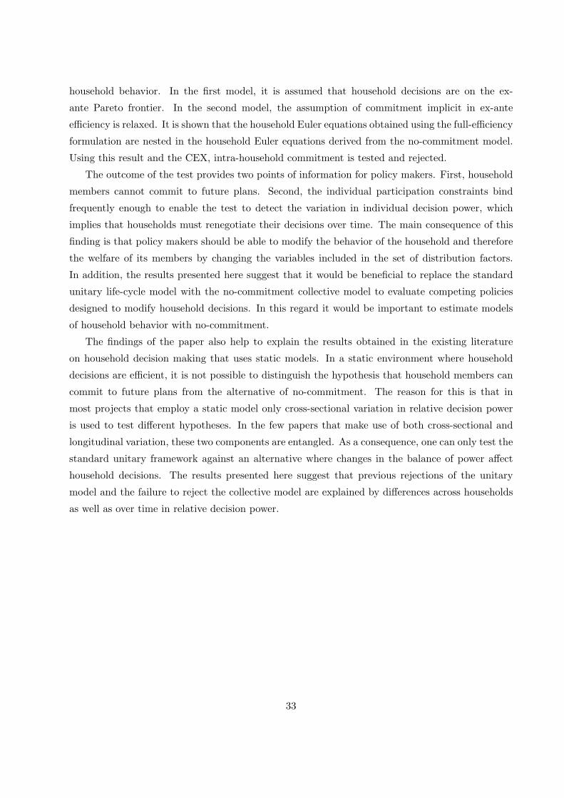
the interaction between consumption growth and the distribution factors. This intuition, which is

depicted in figure 1, clarifies that under ex-ante efficiency only cross-sectional variation can explain

the presence of the distribution factors in the household Euler equations.

Agent 1’s Utility

Agen

t 2’s

Utilit

y

(t,ω’)−Pareto Frontier

Agent 1’s Utility

Agen

t 2’s

Utilit

y

(t+1,ω’’)−Pareto Frontier

−µ(Z’)

−µ(Z’)

−µ(Z’’)

−µ(Z’’)

IndirectEffect

IndirectEffect

Figure 1: Changes in Z and the intra−household allocation with full efficiency.

To distinguish between the full-efficiency and the no-commitment model, a log-linearized version

of the household Euler equations without commitment is derived. Since the estimation of the

collective household Euler equations will be performed restricting the sample to couples with no

changes in marital status, I will assume that for each household there is some surplus to be split

between the two members.

Assumption 2 In each period and state of nature, there exists at least one feasible allocation at

which both agents are better off relative to their reservation utilities.

Under this assumption, Kocherlakota (1996) and Ligon, Thomas, and Worrall (2002) show that

16

in a no-commitment model with two agents at most one agent can be constrained.

One last assumption is required to make the no-commitment household Euler equations com-

parable with the full-efficiency household Euler equations. The following assumption states that

if there is no change in the distribution factors between t and t + 1 and in the two periods the

distribution factors are equal to their expected value, the participation constraints in period t + 1

do not bind. This assumption is required to simplify the derivation of the Euler equations in terms

of consumption growth.16

Assumption 3 If in period t and t + 1 z = E[z] for each z ∈ Z, then λi,t+1 = 0 for i = 1, 2.

Two remarks are in order. First, this assumption is generally satisfied if T is equal to infinity.

With an infinite horizon, if there is no change in the distribution factors between t and t + 1 the

participation constraints will not bind at t + 1, since the value of the reservation utilities does not

change. With a finite time horizon, the participation constraints may bind even though there is no

change in Z if the elapse of time affects differently the value of being married and the value of the

outside options. The assumption is required to rule out this counterintuitive case.

The log-linearized household Euler equations without commitment can now be derived.

Proposition 5 The private household Euler equations for the no-commitment intertemporal col-

lective model can be written as follows:

lnCt+1

Ct= α0 + α1 ln Rt+1 + α2 ln

Qt+1

Qt+

m∑

i=1

αi,3zi lnCt+1

Ct+

m∑

i=1

αi,4zi lnQt+1

Qt

+α5

[(ln

Ct+1

C

)2

−(

lnCt

C

)2]

+ α6

[(ln

Qt+1

Q

)2

−(

lnQt

Q

)2]

+ α7

[ln

Ct+1

Cln

Qt+1

Q− ln

Ct

Cln

Qt

Q

]

+m∑

i=1

α8zi +m∑

i=1

αi,9zi lnCt+1

C+

m∑

i=1

αi,10zi lnQt+1

Q+

∑

i

∑

j

αi,j,11 zizj + RC

(C, Q, Z

)+ ln (1 + et+1,C),

The no-commitment public consumption household Euler equations can be written as follows:

lnQt+1

Qt= δ0 + δ1 ln

Rt+1Pt

Pt+1+ δ2 ln

Ct+1

Ct+

m∑

i=1

δi,3zi lnCt+1

Ct+

m∑

i=1

δi,4zi lnQt+1

Qt

+δ5

[(ln

Ct+1

C

)2

−(

lnCt

C

)2]

+ δ6

[(ln

Qt+1

Q

)2

−(

lnQt

Q

)2]

+ δ7

[ln

Ct+1

Cln

Qt+1

Q− ln

Ct

Cln

Qt

Q

]

+m∑

i=1

δ8zi +m∑

i=1

δi,9zi lnCt+1

C+

m∑

i=1

δi,10zi lnQt+1

Q+

∑

i

∑

j

δi,j,11 zizj + RQ

(C, Q, Z

)+ ln (1 + et+1,Q),

where RC and RQ are Taylor series remainders and eC and eQ are the expectation errors.16 If this assumption is not satisfied the coefficients on log consumption at t and t + 1 differ. The log-linearized

Euler equations will therefore include additional terms that describe the effect of no-commitment at the mean of thedistribution factors.

17


Proposition 5 shows that the distribution factors enter the no-commitment household Euler

equations in three different ways: (i) interacted with consumption growth, (ii) directly and (iii)

interacted with the log of consumption at t + 1. To illustrate the idea behind this result, consider

a change in one of the distribution factors that modifies the individual outside options at t + 1.

Suppose that with this variation in the outside options, at the current intra-household allocation

of resources, the wife is better off as single. If the marriage still generates some surplus, it is

optimal for the couple to renegotiate the allocation of resources to keep the wife from leaving

the household. The optimal renegotiation requires an increase in the wife’s decision power from

M1,t to M1,t+1 = M1,t + λ1,t+1. This renegotiation will modify Ct+1 and Qt+1 relative to the

consumption plan that was optimal before the change in the outside options. This component of

consumption dynamics is captured in the Euler equations by the terms that depend directly on

the distribution factors and by the terms that depend on the interaction between the distribution

factors and consumption at t + 1. This part of consumption dynamics is absent from the efficiency

Euler equations.

To understand the meaning of the terms in the no-commitment Euler equations that depend

on the distribution factors, note that a change in one of the distribution factors has a direct and an

indirect effect as in the full-efficiency case. The direct effect is captured by the change in Mt (Z)

and Mt+1 (Z). Since Mt+1 (Z) = Mt (Z)+λt+1 (Z), the change in the distribution factor generates

the same variation in Mt (Z) in period t and t + 1 and a change in λt+1 (Z) that is specific to

period t+1. As a result, only the latter component of the direct change enters the Euler equations.

This component, which changes the slope of the tangency line at t + 1, is captured by the Euler

equation terms that depend exclusively on the distribution factors. The indirect effect can be

divided into two parts. First, the change in Mt (Z) modifies the allocation of resources to the

two periods and with it the Pareto frontiers. This part of the indirect effect is equivalent to the

full-efficiency case, and it is summarized by the interaction terms between the distribution factors

and consumption growth. Second, the change in λt+1 (Z) generates a change in the Pareto frontier

in period t + 1 in addition to the change that is common to periods t and t + 1. This produces an

additional variation in the tangency point that is captured by the interaction term between the log

of consumption at t + 1 and the distribution factors. This argument is illustrated in figure 2 for

two households with distribution factors Z ′ and Z ′′. The distribution factors are such that for the

first household λ1,t+1 (Z ′) = λ2,t+1 (Z ′) = 0, but for the second one λ1,t+1 (Z ′′) > 0. The previous

discussion indicates that the distribution factors enter the no-commitment Euler equations because

of cross-sectional as well as longitudinal variation.

By means of propositions 4 and 5, it is possible to construct the following test to evaluate the

full-efficiency against the no-commitment intertemporal collective model.

18

Agent 1’s Utility

Agen

t 2’s

Utilit

y

(t+1,ω’’)−Pareto Frontierwith m=−M

1/M

2

Agent 1’s Utility

Agen

t 2’s

Utilit

y

(t,ω’)−Pareto Frontierwith m=−M

1/M

2

m(Z’)

m(Z’)

m(Z’’)

m(Z’’)

Total Effect at t

m(Z’’) −

Figure 2: Changes in Z and the intra−household allocation with no commitment.

M2(Z’’)

λ1(Z’’)

Total Effect at t+1

TEST OF COMMITMENT. Under the assumption of ex-ante efficiency, the distribution

factors should enter the household Euler equations only as interaction terms with private and public

consumption growth. If no-commitment is a correct specification of household intertemporal behav-

ior, the distribution factors should enter household Euler equations not only as interaction terms

with consumption growth, but also directly and interacted with consumption at t + 1.

Since the full-efficiency household Euler equations are nested in the no-commitment household

Euler equations, this test can be performed using standard methods. The outcome of the test will

establish whether it is worth investing in public policies whose main goal is to change household

decisions by modifying the decision power of individual household members.

5 Implementation of the Test

The test of commitment requires a set of distribution factors that are common to the full-efficiency

and no-commitment model. Potential candidates are the wife’s and husband’s income in period

t + 1. To see this, consider first the full-efficiency model. In this model, the relative decision power

µ varies with the wife’s and husband’s probability distribution of income at the time of marriage.

Consider the no-commitment model. In this case the change in decision power from Mt to Mt+1

depends on the wife’s and husband’s probability distribution of income at the time of marriage as

well as on the actual realizations of individual incomes at t + 1. As a result, in the full-efficiency

model the wife’s and husband’s income in period t + 1 should enter the Euler equations as a proxy

for the probability distributions of individual income at the time of household formation. In the no-

commitment model, the realizations of individual income at t + 1 should enter the Euler equations

because they affect the change from Mt to Mt+1 and as a proxy for the probability distributions

19

of individual income at the time of marriage. The test will determine the role of the wife’s and

husband’s income in the household Euler equations.

Two caveats related to the choice of the distribution factors should be discussed. First, the

econometrician does not know which variables are distribution factors. Suppose that the no-

commitment or the efficiency model is correct. Suppose also that the test is implemented using

variables that are not distribution factors. The test will then reject the no-commitment or efficiency

model in favor of the unitary model. To explain the second caveat, suppose that the realizations

of income at t + 1 are a poor proxy of the probability distributions of income at the time of house-

hold formation. Suppose also that the correct model of household intertemporal behavior is the

full-efficiency model. This model will generally be rejected in favor of the unitary model because

the relative decision power at the time of marriage is independent of the income realizations at

t + 1. However if the correct framework is the no-commitment model, the full-efficiency and uni-

tary model will be rejected in favor of no-commitment as long as the realizations of income belong

to the set of distribution factors.

Using a recursive formulation of the no-commitment model it can be shown that the individual

decision power at t+1 should depend not only on the individual income realizations in period t+1,

but also on household savings in period t. In this paper it is assumed that household savings is

not a distribution factor. To be consistent with this assumption, the test will be first performed

by excluding savings from the Euler equations. Subsequently, to provide evidence on assumption

1, the test will be implemented controlling for savings.

The commitment hypothesis is tested using the distance statistic approach developed by Newey

and West (1987). The test is implemented in three steps. First, the no-commitment Euler equations

are estimated using the Generalized Method of Moments (GMM). Second, the no-commitment

Euler equations are estimated using GMM and imposing the restrictions required to obtained the

full-efficiency Euler equations. Finally, the distance statistic is computed. In both the first and

second steps, I use the efficient weighting matrix of the unconstrained model.

6 Data

Since 1980 the CEX survey has been collecting data on household consumption, income, and

different types of demographics. The survey is a rotating panel organized by the Bureau of Labor

Statistics (BLS). Each quarter about 4,500 households, representative of the U.S. population, are

interviewed: 80 percent are reinterviewed the following quarter, while the remaining 20 percent

are replaced by a new randomly selected group. Each household is interviewed at most for four

quarters and detailed information is collected on expenditures, demographics, and income. The

data used in the estimation cover the period 1982-1995. The first two years are excluded because

20

the data were collected with a slightly different methodology.

Total private consumption is computed as the sum of food at home, food away from home,

tobacco, alcohol, public and private transportation, personal care, and clothing of wife and husband.

Total public consumption is defined as the sum of maintenance, heating fuel, utilities, housekeeping

services, repairs, and children’s clothing.17 Private and public consumption are deflated using a

weighted average of individual price indices, with weights equal to the expenditure share for the

particular consumption good. The numeraire is defined to be private consumption.

Individual income is the sum of the components that can be imputed to each member, i.e.,

income received from non-farm business, income received from farm business, wage and salary

income, social security checks and supplemental security income checks for the year preceding the

interview. The real interest rate is the quarterly average of the 20-year municipal bond rate deflated

using the household-specific price index.

The CEX collects data on financial wealth, which enables one to recover household savings

during the first and last quarter of the interview year. In particular, saving in the last quarter is

defined as the amount of wealth the household had invested the last day of the last quarter of the

interview year in savings accounts, U.S. savings bonds, stocks, bonds, and other securities. Savings

in the first quarter is defined as savings in the last quarter minus the difference in amount held

in savings accounts, U.S. savings bonds, stocks, bonds, and other securities on the last day of the

fourth quarter of the interview year relative to a year ago. Savings in the second and third quarter

are then imputed using average savings in the first and fourth quarter.

Rather than employ the short panel dimension of the CEX, I follow Attanasio and Weber (1995)

and use synthetic panels. The commitment test can be implemented using synthetic panels because

the equations to be estimated are linear in the parameters. The panels are constructed for married

couples using the year of birth of the husband and the following standard method. All households

are assigned to one of the cells that are formed using a 7-year interval for the year of birth. The

variables of interest are then averaged over all the households belonging to a given cohort observed

in a given quarter. To avoid unnecessary overlapping between quarters, for each household in each

quarter, I use only the consumption data for the month preceding the interview and drop the data

for the previous two months.

To construct the synthetic cohorts, I exclude from the sample singles, rural households, house-

holds with incomplete income responses, and households experiencing a change in marital status.

Only cohorts for which the head’s age is between 21 and 60 are included in the estimation. Cohorts

with size smaller than 150 are dropped. Table 1 contains a description of the cohorts. Table 217 It is likely that food away from home and private transportation contain a public component. Moreover, food

consumed by children is included in food at home. Since it is not possible to distinguish between the private and thepublic component, and these items are mostly private consumption, they are included in private consumption.

21

reports the summary statistics for the CEX sample.

7 Econometric Issues

The residuals of the collective Euler equations contain the expectation error implicit in these in-

tertemporal optimality conditions. Since part of the expectation error is generated by aggregate

shocks, it could be correlated across households. This implies that the Euler equations can be

consistently estimated only if households are observed over a long period of time, as suggested

by Chamberlain (1984). One of the main advantages of using synthetic panels is that cohorts are

followed for the whole sample period. This should reduce the effect of aggregate errors on the

estimation results.

Under the assumption of rational expectations, any variable known at time t should be a valid

instrument in the estimation of the Euler equations by GMM. The existence of measurement errors,

however, may introduce dependence between variables known at time t and concurrent and future

variables, even under rational expectations. To address this problem, only variables known at t− 1

are used.

The test is implemented using only couples with no change in marital status. This selection of

the sample may introduce selection biases. Mazzocco (2005) estimates household Euler equations

after controlling for selection into marriage and selection into households with no change in marital

status. Since in Mazzocco (2005) there is no evidence of selection biases, the test will be performed

without the addition of selection terms.

A controversial assumption made in this paper, and more generally in papers estimating Euler

equations, is that household consumption is strongly separable from leisure. In this paper, the

nonseparability between consumption and leisure is not formally modeled. Following Browning

and Meghir (1991), Attanasio and Weber (1995), and Meghir and Weber (1996), however, the

effect of leisure on consumption decisions will be captured by modeling the leisure variables as

conditioning variables, i.e., variables that may affect preferences over the good of interest, but

which are not of primary interest. In particular, following Meghir and Weber (1996), the test will

be performed by adding as conditioning variables the change in a dummy equal to 1 if the wife

works and the change in a similar dummy for the husband. The test has also been performed

by adding the previous dummy for the wife and the wife’s leisure growth. Since the results are

identical, I only report the outcome of the test obtained using the first set of labor supply variables.

To allow for observed heterogeneity, I follow Attanasio and Weber (1995) and estimate the full-

efficiency and no-commitment Euler equations including family size, number of children, number

of children younger than 2, and three seasonal dummies.

Given the longitudinal nature of the CEX data, it is crucial to allow each household to have

22

a different and unrestricted covariance structure. To that end, the covariance matrix is computed

using the efficient weighting matrix in the GMM procedure. In particular, denote by E [gi (θ)] the

set of moment conditions, where θ is the vector of parameters to be estimated. Let Ω = E [gig′i]

and G = E

[∂

∂θ′gi (θ)

]. Following Hansen (1982), under general regularity conditions,

√n

(θ − θ

)

converges in distribution to a normal with mean zero and covariance(G′Ω−1G

)−1. The covariance

matrix is then estimated replacing Ω with Ω =1n

∑i gig

′i and G with G =

1n

∑i

∂

∂θ′gi, where

gi = gi

(θ). As suggested by Wooldridge (2002), this covariance matrix is general enough to allow

for heteroskedasticity and arbitrary dependence in the residuals.

8 Results

Tables 3 and 4 report the results for the commitment test.18 The two tables have a similar structure.

The first two columns report the estimates of the private and public Euler equation coefficients for

the no-commitment model. The third and fourth columns contain the coefficient estimates when

the coefficients on the no-commitment terms are constrained to be zero. The last two columns have

been added to further test the collective model against the unitary framework. They report the

private and public Euler equation estimates when all the distribution factor terms are constrained

to be zero. The outcome of the commitment test is reported in the first row of the tables.

The full-efficiency model and therefore the standard unitary framework are rejected at any

standard significance level. The rejection should be attributed to both husband’s and wife’s in-

come, since both distribution factors enter significantly into the private and public Euler equations

directly, interacted with consumption growth, and interacted with consumption at t + 1. The

no-commitment test has also been implemented after controlling for household savings at t. The

outcome of the test, which is reported in table 4, is identical to the outcome obtained without

controlling for household savings.

Since the no-commitment model is not rejected, the estimated coefficients can be used to de-

termine the effect of a change in relative decision power on consumption dynamics. This effect

can be calculated by computing the derivative of consumption growth with respect to the wife’s

and husband’s income. These derivatives can be computed at different points. I will describe the

derivatives at the following two points: at mean individual income, mean consumption, and hence

zero consumption growth; at the median of consumption growth, log consumption, and individual

income. The first point is chosen because the derivatives are straightforward to compute since they

correspond to the coefficients on the wife’s and husband’s income. The second point is considered18 The test has also been implemented using the PSID with data on food consumption. The outcome of the test

does not change and is available at http://www.ssc.wisc.edu/∼mmazzocc/research.html.

23

to determine the effect of the other coefficients that depend on individual income. Since the results

with and without savings are similar I will only use the coefficients in table 3. I will first discuss

the derivatives of household private consumption growth. The derivative with respect to the wife’s

income at the first point is negative and equal to -0.0312. The derivative with respect to the hus-

band’s income is positive and equal to 0.0244. To interpret the two derivatives consider an increase

in the wife’s and husband’s quarterly income by 1,000 dollars. This increase corresponds to a shift

from the median to the 64th percentile of the empirical distribution for the wife’s income and to a

shift from the median to the 60th percentile for the husband’s income. The first derivative implies

that the increase in the wife’s income reduces private consumption growth from zero to -0.0312. To

provide some insight on the size of the change, observe that a rate of growth of zero corresponds

to the 49th percentile of the empirical distribution and a rate of growth of -0.0312 to the 30th

percentile. According to the second number the addition of 1,000 dollars to the husband’s income

increases private consumption growth from zero to 0.0244, where 0.0244 corresponds to the 65th

percentile. The derivative calculated at the second point is equal to -0.0836 for the wife’s income

and to 0.0329 for the husband’s income. Thus, the effect of a change in income has an even larger

effect if computed at the median.

The derivative of public consumption growth with respect to the wife’s and husband’s income

have the opposite sign at both points. At the first point the derivative is equal to 0.0248 for

the wife’s income and to -0.0216 for the husband’s income. This implies that an increase in the

wife’s income by 1,000 dollars increases public consumption growth from zero to 0.0248, where

zero growth corresponds to the 49th percentile of the empirical distribution and a growth of 0.0248

corresponds to the 63rd percentile. An increase in the husband’s income by the same amount shifts

public consumption growth from the 49th percentile to the 36th percentile. The derivative at the

second point is equal to 0.0650 for the wife’s income and to -0.0300 for the husband’s income. As

for private consumption, at the median the effect of a change in individual income has a larger

effect on consumption dynamics.

Three features of the results should be emphasized. First, changes in the wife’s and husband’s

income have opposite effects on consumption growth. Second, the size of these effects is substantial.

Third, changes in individual income have the opposite effect on private and public consumption

growth. These features are consistent with a set of households with the following four character-

istics. First, each household is characterized by no-commitment and an increase in one spouse’s

income increases her decision power. Second, the wife is more risk averse than the husband. Third,

the wife cares more about public consumption relative to the husband. Fourth, the discount fac-

tor multiplied by the gross interest rate is larger than one in most periods, which implies that

individuals would rather choose an increasing consumption path. To understand why this set of

households is consistent with the findings of this paper note that no-commitment and the hetero-

24

geneity in preferences produce two distinct effects. First, if the wife is more risk averse than the

husband, an increase in her decision power increases household savings because of precautionary

reasons and consumption smoothing. This and the preferences for increasing consumption paths

imply that private and public consumption growth will be lower. Second, the heterogeneity in

preferences for public consumption implies that an increase in the wife’s relative decision power

at t + 1 shifts resources from private to public consumption at t + 1. Thus, the rate of growth of

public consumption will increase and the rate of growth of private consumption will decrease. The

results presented in this section require that the latter effect is strong enough.

The type of preference heterogeneity that is required to explained the estimated coefficients is

consistent with the empirical evidence described in the literature on household behavior. A couple

of recent papers have estimated the risk aversion of wives and husbands separately. The estimates

in both Dubois and Ligon (2005) and Mazzocco (2005) suggest that wives are more risk averse

than husbands. There is also a general agreement that wives care more about public consumption

especially if the consumption of children is included in it, as suggested for instance by Thomas

(1990). There are also several papers that have estimated discount factors that multiplied by the

gross interest rates used in the estimation are larger than one. In the data the realized real annual

interest rate is above 4.8 for all households except the bottom 1%. This implies that any annual

discount factor above 0.954 would work. Moore and Viscusi (1990) and Lawrance (1991) are two

examples of papers that estimate discount factors that are above that threshold.19

One additional point deserves discussion. This paper clarifies that labor supply and income

variables affect household decisions in at least two ways: (i) through preferences if leisure is non-

separable from other consumption goods and (ii) through the individual decision power. The

labor force participation dummies are added to the Euler equations to consider the potential non-

separability between consumption and leisure. The estimation results indicate that the effect of

the labor dummies declines significantly when the distribution factors are properly modeled. In

particular, in the standard unitary model the effect of changes in relative decision power is not

considered and the coefficients on the labor dummies are large and significant. In the efficiency

model only the cross-sectional variation in relative decision power is taken into account and the

husband’s and wife’s labor dummies have still a significant effect on consumption growth. When

the cross-sectional and longitudinal variation in the balance of power is considered, however, the

coefficients on the labor dummies become smaller and insignificant. This suggests that previous

studies may have overestimated the effect of non-separability between consumption and leisure on

household decisions, since the effect of no-commitment was not considered.19 The results presented in this section are also consistent with a set of households in which the husband is more

risk averse and cares more about private consumption. However, Dubois and Ligon (2005) and Mazzocco (2005)reject this type of heterogeneity.

25

9 Evidence From Simulated Data

The goal of this section is to establish whether lack of commitment can explain qualitatively and

quantitatively the empirical patterns discussed in the previous section. This is achieved by simu-

lating the no-commitment model.

This section is divided into three parts. The next subsection describes the simulation of house-

hold behavior. The second subsection analyzes the effect of no-commitment on household intertem-

poral behavior using the simulated data. The last subsection discusses two alternative models that

may explain the presence of income variables in the Euler equations.

9.1 Simulation

The no-commitment model is simulated using a recursive formulation of problem (6). The reserva-

tion utility for a married individual is the value of being single for one period and making optimal

decisions from that period onward.20 The simulation requires assumptions about individual pref-

erences and about the probability distributions from which individual incomes are drawn. It also

requires the discretization of the state variables.

The individual utility functions are assumed to have the following form:

ui(ci, Q

)=

[(ci

)σi (Q)1−σi

]1−γi

(1− γi),

with γi > 0 and 0 < σi < 1. The parameter γi captures the intertemporal aspects of individual pref-

erences. In particular, −1 /γi is agent i’s intertemporal elasticity of substitution, which measures

the willingness to substitute the composite good C =(ci

)σi (Q)1−σi between different dates. The

parameter σi captures the intraperiod features of individual preferences and it measures in each

period the fraction of expenditure assigned to agent i which is allocated to private consumption.

In Mazzocco (2005) the intertemporal elasticity of substitution is estimated separately for

women and men using the CEX. It is found that γ is around 2.5 for men and 4.5 for women.

These values are adopted in the simulation.21 To the best of my knowledge, no paper has esti-

mated the parameter σ separately for women and men. Since the empirical evidence suggests that

women care more about public consumption, it is assumed that σ is equal to 0.5 for women and to

0.6 for men. As discussed in the empirical section, since women are more risk averse than men the

choice of a smaller σ for women is crucial to be able to replicate the estimation results obtained

with the CEX.20 The derivation of the recursive formulation for the no-commitment model is based on Marcet and Marimon

(1998) and is discussed in Lucas, Mazzocco, Yamaguchi (2005).21 Dubois and Ligon (2005) estimate the ratio of the wife’s γ to the husband’s using data from the Philippines.

Their estimated ratio is around 1.5. Given that the estimates in Dubois and Ligon (2005) and Mazzocco (2005) areobtained using different datasets, the estimated ratio is remarkably similar.

26

Simulating the model requires the distribution of income conditional on individual character-

istics. The distribution is estimated under the assumption that individual income is log-normally

distributed. In the data individual income is reasonably persistent. In the estimation this feature is

captured by allowing the conditional distribution to depend on income in the previous period. It is

assumed that lagged income is the only variable affecting the income process. Under these assump-

tions, the conditional distribution can be estimated using the CEX and a standard regression. The

distributions for women and men are estimated separately. The top and bottom 5% of the income

distribution is dropped. The mean of the distribution is the fitted value of the income equation

evaluated at lagged income, and the variance is the estimated variance of the corresponding error

term. The constant in the regression of quarterly log real income on lagged quarterly log real

income for women is equal to 1.42, whereas it is equal to 1.72 for men. The coefficient on lagged

log income is equal to 0.82 for women and 0.79 for men. This implies that men draw income from a

better distribution. It also implies that the income process of men and women is highly and equally

persistent: a 100% increase in lagged income is associated with an 80% increase in current income.

The estimated standard deviation of the income process is larger for women at 0.41 relative to a

standard deviation of 0.36 for men. The continuous distribution is then optimally discretized using

proposition 1 in Kennan (2004), which shows that the best approximation F to a given distribution

F using a fixed number of grid points xini=1 is given by F (xi) = (F (xi+1) + F (xi)) /2 for i < n

and F (xn) = 1.

To simulate household intertemporal behavior one has to discretize the state variables. The set

of state variables is composed of household savings, individual incomes, and relative decision power.

The choice of the grid for household savings is of particular importance. If the grid is too coarse,

the household Euler equations will not be satisfied. Household savings for a married couple are

therefore described using a 53-point grid, the lowest and highest points being, respectively, -8,000

dollars and 62,000 dollars. This range is chosen to reflect the distribution of financial assets in the

CEX, where about 1% of households report an asset level below the chosen range and 3% above.

The first 4 points and the last 15 are equally spaced and 2,000 dollars apart. The remaining points

are equally spaced and 1,000 dollars apart. The grid for singles corresponds to the grid for married

individuals except that each point is divided by two. I have experimented with fewer grid points,

but in those simulations the household Euler equations are not a good approximation of household

intertemporal behavior.

The grid for individual quarterly income is composed of 4 points. They are set equal to the

20th, 40th, 60th, and 80th percentile of the empirical distribution of men’s and women’s income.

The corresponding grid for women is $800, $1,657, $2,930, and $4,601. The grid for men is $1,709,

$3,126, $4,910, and $7,078. The conditional probability of each point is computed by applying

Kennan’s proposition to the logarithm of the grid points.

27

The grid for individual decision power requires a separate discussion. In the simulation, the

individual decision power is normalized to be between zero and one by dividing the decision power

of each spouse by the sum. This normalization simplifies the simulation in two ways. First, the

set of state variables includes only the decision power of one spouse. Second, the decision power

of this spouse can be easily discretized. The grid is composed of 21 points: .01, .05, .10, ..., .90,

.95, and .99. I have tested the robustness of the simulation with respect to changing the number

of grid points. The results indicate that it is important to use a reasonably fine grid. With a grid

that is too coarse, there are mutually beneficial marriages that do not occur because the grid does

not contain any points within the range of Pareto weights for which the marriage is sustainable.

The no-commitment model is simulated for 25 consecutive quarters for 10,000 households.

Afterwards each individual receives a fixed level of utility. This assumption imposes a restriction

on individual behavior. But it enables me to use a finer grid for savings and individual decision

power. To increase the number of periods I would have to reduce the number of points in the

savings grid or decision power grid. Initial savings is set equal to 10,000 dollars, which corresponds

to the midpoint of the savings grid.

The price of private and public consumption corresponds to the average by quarter of the

household specific price indices. The interest rate in each quarter is the quarterly average of the

20-year municipal bond rate used with the CEX data. The yearly discount factor is set equal to

0.96. It corresponds to a quarterly discount factor of 0.99 and it implies that βRt > 1 for every

realization of the interest rate in the simulation. Thus, everything else equal, an individual would

rather have an increasing consumption path. The first of the 25 periods corresponds to the first

quarter of 1982, which is the first quarter used in the empirical section.

9.2 Results

This section discusses the effect of lack of commitment on household intertemporal behavior for

married households. The discussion will be divided into two parts. The first part presents some

descriptive evidence on the effect of changes in individual decision power on household behavior

using simple regressions. The second part reports the results of the no-commitment test obtained

using simulated data.

In the simulated data the average wife’s decision power is similar to the husband’s and equal

to 0.49. All but 1% of married couples experience a change in relative decision power during the

sample period. Table 5 reports four sets of regression coefficients obtained by regressing (i) the

husband’s relative decision power on the husband’s and wife’s income, (ii) household savings at t

on the initial husband’s decision power at t and the change in his decision power, (iii) household

private consumption at t on the initial husband’s decision power at t and the change in his decision

28

power, (iv) public consumption at t on the initial husband’s decision power at t and the change in

his decision power. In the simulated data household savings and consumption are characterized by

a time trend. Moreover, household decisions differ depending on the amount of resources available

at the beginning of the period. For this reason, the regression coefficients are estimated after

controlling for time dummies and time dummies interacted with total resources at the beginning

of the period, i.e., household income plus initial savings. The coefficients should therefore be

interpreted as the average effect across periods of the regressors. Savings, consumption, and income

variables are divided by 1,000 dollars. Since the sum of individual decision power is normalized to

1, in the following discussion an increase in the husband’s decision power corresponds to a reduction

in the wife’s.

One caveat of the regression analysis must be discussed. The relationships between the de-

pendent and independent variables are generally non-linear and the majority of the regressors are

endogenous. Consequently, the regression results should be interpreted as descriptive evidence of

the effect of changes in relative decision power on household intertemporal behavior. They should

not be considered the outcome of the estimation of structural relationships.

The first part of Table 5 reports the effect of changes in individual income on the relative

decision power. The results indicate that an increase in the wife’s income has the intuitive effect of

reducing the husband’s decision power and hence increasing hers with a coefficient of -0.066. The

husband’s income has the opposite effect with a coefficient of 0.065. This implies that an increase

in the wife’s income by 1,000 dollars reduces the husband’s decision power by 0.066, which at the

mean corresponds to a reduction of 13%. A similar change in the husband’s income increases his

decision power by the same percentage.

The second part of Table 5 describes the effect of a change in relative decision power on saving

decisions conditional on initial resources. As discussed in the empirical section, since women are

more risk averse, everything else equal they prefer smoother consumption paths and would rather

accumulate larger amounts of precautionary savings relative to men. This has two main implica-

tions. First, in a cross-section of households, holding everything else constant, households in which

the wife has larger decision power should save more. Second, if the same household is followed

over time, holding everything else constant, an increase in the wife’s decision power should increase

household savings. The estimated coefficients are consistent with these implications. The coeffi-

cient on initial decision power is -1.383, whereas the coefficient on the change in decision power is

-0.588. To provide an economic interpretation of the first coefficient, consider two households that

are identical except that household 1 is dominated by the wife, whereas household 2 is dominated

by the husband. The estimated coefficient indicates that if household 1 has accumulated 14,000

dollars in wealth, household 2 saves 10% less, where 14,000 dollars correspond to the first quartile

of the simulated wealth distribution. At the median, which corresponds to 21,000 dollars, the hus-

29

band dominated household saves 6.6% less. At the third quartile it saves 5% less, where the third

quartile is 28,000 dollars. The coefficient on the change in decision power indicates that the effect

of longitudinal variation in the balance of power on savings is slightly less than half the effect of

the cross-sectional variation.

The third part of Table 5 reports the estimated coefficients obtained by regressing household

private consumption on the husband’s initial decision power and its change. The heterogeneity in

preferences implies that a shift in the balance of power in favor of the husband should increase

private consumption for two reasons. First, because men are less risk averse, an increase in their

decision power reduces savings and increases the amount of resources consumed by the household.

Second, because men care more about private consumption, a shift in decision power in favor of the

husband increases the amount of resources allocated to private consumption. The estimation results

are consistent with this argument. The coefficient on initial decision power is 1.131, whereas the

coefficient on the change is 0.669. The first number implies that private consumption in a household

that is dominated by the husband is equal to private consumption of a household that is dominated

by the wife plus 1,131 dollars. At the mean this corresponds to an increase of 24%. The coefficient

on the change in decision power indicates that the longitudinal variation has about half the effect

of the cross-sectional variation in decision power.

The fourth part of Table 5 describes the relationship between public consumption and relative

decision power. In this case, the heterogeneity in risk aversion and the heterogeneity in preferences

for public consumption have opposite effects. As for private consumption, a shift in decision power

in favor of the husband implies that the household saves less and consumes a larger amount of

resources. The heterogeneity in σ, however, has the contrary effect. The two opposite effects are

reflected in the estimated coefficients. The coefficient on initial decision power is smaller than

the one estimated for private consumption and equal to 0.252. At the mean it corresponds to an

increase of 7%. The longitudinal variation in decision power has a negative effect with a coefficient

of -0.081. At the mean this is equivalent to a reduction in public consumption of 3%.

The simulated data are then used to perform the no-commitment test. The results are reported

in Table 6. The distance statistic indicates that the efficiency and unitary model are strongly

rejected. The size and statistical significance of the coefficients that capture the effect of the

longitudinal variation in relative decision power explain the rejection.

I will now discuss the derivative of consumption growth with respect to the wife’s and husband’s

income. The derivatives can be used to determine whether the no-commitment model can explain

the empirical findings obtained using the CEX. I will consider the derivatives at the two points that

were used with the CEX: at mean individual income, mean consumption, and zero consumption

growth; at the median of consumption growth, log consumption, and individual income. I will first

discuss the derivatives of private consumption growth. At the first point the derivative with respect

30

to the wife’s income is -0.034. This implies that an increase in the wife’s income by 1,000 dollars

reduces private consumption growth from zero to -0.034. To provide some insight on the size of the

effect note that a rate of growth of zero corresponds to the 47th percentile and a rate of growth

of -0.034 to the 25th percentile. The derivative obtained using the simulated data has therefore

identical sign and size that is similar to the one computed using the CEX data. The derivative

with respect to the husband’s income is 0.0083. This means that an increase in the husband’s

income by 1,000 dollars increases private consumption growth from zero to 0.0083, where 0.0083

corresponds to the 51st percentile. The sign of the derivative is therefore the same as for the CEX

data, but the magnitude of the effect is smaller. At the second point, the derivative with respect

to the wife’s income is still negative and similar in size at -0.030. As a result, an increase in the

wife’s income by one thousand dollars shifts consumption growth from the median, which is equal

to 0.0046, to the 27th percentile. The derivative with respect to the husband’s income is positive

and equal to 0.028. In this case consumption growth shifts from the median to the 58th percentile.

Thus, at the second point, the effect of a change in individual income has the same sign as in the

CEX data. Moreover, the magnitude of the effect is closer to the one measured in the CEX also

for the husband’s income.

The derivative of public consumption with respect to husband’s and wife’s income have the

same sign, but a magnitude that is smaller than the derivatives obtained using the CEX. At the

first point, the derivative is equal to 0.014 with respect to the wife’s income and to -0.0017 with

respect to the husband’s income. The first value indicates that an increase in the wife’s income by

1,000 dollars shifts the rate of growth from zero, which corresponds to the 49th percentile, to the

55th percentile. The second value implies that the same change in the husband’s income modifies

the growth rate from zero to the 47th percentile. At the second point the derivative is equal to

0.019 for the wife’s income and to -0.008 for the husband’s income. In this case a change in the

wife’s income by 1,000 dollars produces a shift from the median, which corresponds to 0.0015, to

the 57th percentile. The same change in the husband’s income shifts the rate of growth from the

median to the 42nd percentile.

9.3 Alternative Hypotheses

The simulation results presented in this section show that the no-commitment model can explain

the sign of the effect of changes in income on consumption growth observed in the CEX. The

magnitude of the effect is also consistent with the size measured in the CEX. The only exception is

the effect of changes in income on public consumption growth, which is smaller in the simulation.

There are, however, other models that may explain the presence of income variables in the

household Euler equations even after controlling for labor supply variables. The two main alterna-

31

tives are the unitary model with borrowing constraints and an efficiency model with asymmetric

information about individual income.22 The test proposed in this paper is not meant to rule out

these alternative hypotheses. Intuitively, borrowing constraints and asymmetric information should

explain part of the variation in consumption dynamics.

The evidence presented in this paper suggests, however, that the unitary model with borrowing

constraints and the efficiency model with asymmetric information cannot explain by themselves

the effect of individual income on consumption growth. To see this note that the unitary model

with borrowing constraints predicts that an increase in the wife’s income as well as an increase

in the husband’s income should increase consumption growth. The results presented here indicate

that the wife’s and husband’s income have opposite effects on consumption growth, which implies

that borrowing constraints cannot be the only explanation for the relationship between individual

income and consumption growth.

The alternative hypothesis of asymmetric information deserves a separate discussion. Wang

(1995) has shown that in an environment in which two individuals consume only private goods

and cannot observe the realizations of each other’s income, individual consumption is positively

correlated with individual income holding constant aggregate income. This implies that individual

consumption is positively correlated with individual income even if one holds the partner’s income

constant. Intuitively, a similar result should apply to a model with public consumption. Consider

an increase in the wife’s income at t + 1 holding the husband’s income constant. Wang’s result

implies that private consumption of the wife at t + 1 should increase. Under standard assumptions

on preferences, since the husband’s income has not changed, his private consumption should not

decrease. Therefore, intuitively, in an environment with asymmetric information an increase in

the wife’s income at t + 1 should increase private consumption growth. This result contradicts the

finding of this paper that an increase in the wife’s income holding the husband’s income constant re-

duces private consumption growth. Consequently, an efficiency model with asymmetric information

cannot be the only explanation for the presence of income variables in the Euler equations.

An interesting research project is a project that attempts to disentangle and quantify the effect

of no-commitment, borrowing constraints, and asymmetric information on household intertemporal

decisions. This is, however, beyond the scope of this paper and left for future research.

10 Conclusions

In this paper, two models of household intertemporal behavior are considered to understand the link

between intra-household commitment, family decisions, and social programs designed to change22 See for instance Atkeson and Lucas (1992), Wang (1995), and Ligon (1998) for a discussion of efficiency models

with asymmetric information.

32

household behavior. In the first model, it is assumed that household decisions are on the ex-

ante Pareto frontier. In the second model, the assumption of commitment implicit in ex-ante

efficiency is relaxed. It is shown that the household Euler equations obtained using the full-efficiency

formulation are nested in the household Euler equations derived from the no-commitment model.

Using this result and the CEX, intra-household commitment is tested and rejected.

The outcome of the test provides two points of information for policy makers. First, household

members cannot commit to future plans. Second, the individual participation constraints bind

frequently enough to enable the test to detect the variation in individual decision power, which

implies that households must renegotiate their decisions over time. The main consequence of this

finding is that policy makers should be able to modify the behavior of the household and therefore

the welfare of its members by changing the variables included in the set of distribution factors.

In addition, the results presented here suggest that it would be beneficial to replace the standard

unitary life-cycle model with the no-commitment collective model to evaluate competing policies

designed to modify household decisions. In this regard it would be important to estimate models

of household behavior with no-commitment.

The findings of the paper also help to explain the results obtained in the existing literature

on household decision making that uses static models. In a static environment where household

decisions are efficient, it is not possible to distinguish the hypothesis that household members can

commit to future plans from the alternative of no-commitment. The reason for this is that in

most projects that employ a static model only cross-sectional variation in relative decision power

is used to test different hypotheses. In the few papers that make use of both cross-sectional and

longitudinal variation, these two components are entangled. As a consequence, one can only test the

standard unitary framework against an alternative where changes in the balance of power affect

household decisions. The results presented here suggest that previous rejections of the unitary

model and the failure to reject the collective model are explained by differences across households

as well as over time in relative decision power.

33

References

[1] Apps, Patricia F. and Ray Rees: “Taxation and the Household,” Journal of Public Economics,35, no. 3 (April 1988): 355-369.

[2] Ash, R. B.: Real Analysis and Probability, New York, Academic Press (1972).

[3] Atkeson, Andrew and Robert E. Lucas: “On Efficient Distribution with Private Information,”The Review of Economic Studies, 59, no. 3 (July 1992): 427-453.

[4] Attanasio, Orazio P. and Hamish Low: “Estimating Euler Equations,” Review of EconomicDynamics, 7, no. 2 (April 2004): 406-435.

[5] Attanasio, Orazio, Costas Meghir, and Ana Santiago: “Education Choices in Mexico: Usinga Structural Model and a Randomized Experiment to Evaluate Progresa,” Center for theEvaluation of Development Policies Working Paper (2001).

[6] Attanasio, Orazio P. and Jose Victor Rios Rull: “Consumption Smoothing and ExtendedFamilies,” University College of London Working Paper (July 2000).

[7] Attanasio, Orazio P. and Guglielmo Weber: “Is Consumption Growth Consistent with In-tertemporal Optimization? Evidence from the Consumer Expenditure Survey,” Journal ofPolitical Economy, 103, no. 6 (1995): 1121-1157.

[8] Aura, Saku: “Uncommitted Couples: Some Efficiency and Policy Implications of MaritalBargaining,” Manuscript, University of Missouri-Columbia (2004).

[9] Basu, Kaushik:“Gender and Say: A Model of Household Behavior with Endogenously-Determined Balance of Power,” Economic Journal, forthcoming.

[10] Behrman, Jere, Pilali Segupta, and Petra Todd: “Progressing Through Progresa: An ImpactAssessment of a School Subsidy Experiment,” Penn Institute for Economic Research, ResearchPaper Series (2001).

[11] Blundell, R., P. A. Chiappori, T. Magnac, and C. Meghir: “Collective Labor Supply: Hetero-geneity and Nonpartecipation,” Institute for Fiscal Studies Working Paper (2001).

[12] Browning, Martin, Francois Bourguignon, Pierre-Andre Chiappori, and Valerie Lechene: “In-come and Outcomes: A Structural Model of Intrahousehold Allocation,” Journal of PoliticalEconomy, 102, no. 6 (December 1994): 1067-1096.

[13] Browning, Martin and Annamaria Lusardi: “Household Savings: Micro Theories and MicroFacts,” Journal of Economic Literature, 34 (December 1996): 1797-1855.

[14] Browning, Martin and Costas Meghir: “The Effects of Male and Female Labor Supply onCommodity Demands,” Econometrica, 59, no. 4 (July 1991): 925-951.

[15] Carroll, Christopher D.: “Death to the Log-Linearized Consumption Euler Equation! (AndVery Poor Health to the Second-Order Approximation),” Advances in Macroeconomics, 1, no.1, Article 6 (2001).

[16] Chamberlain, Gary: “Panel Data,” The Handbook of Econometrics, 2, edited by Zvi Grilichesand Michael D. Intriligator, New York, North-Holland (1984).

[17] Chiappori, Pierre-Andre: “Rational Household Labor Supply,” Econometrica, 56 (January1988): 63-90.

34

[18] Chiappori, Pierre-Andre: “Collective Labor Supply and Welfare,” Journal of Political Econ-omy, 100, no. 3 (1992): 437-467.

[19] Davis, Lucas, Maurizio Mazzocco, and Shintaro Yamaguchi: “Labor Supply, Wealth Dynamicsand Marital Decisions,” Working Paper, Department of Economics, University of Wisconsin(2005).

[20] Dubois, Pierre and Ethan Ligon: “Incentives and Nutrition for Rotten Kids: IntrahouseholdFood Allocation in the Philippines,” Manuscript, University of California, Berkeley (2005).

[21] Duflo, Esther and Christopher Udry: “Intrahousehold Resource Allocation in Cote D’Ivore:Social Norms, Separate Accounts and Consumption Choices,” NBER Working Paper, (May,2004).

[22] Gobert, Karine and Michel Poitevin: “Non-commitment and Savings in Dynamic Risk-sharingContracts,” Economic Theory, 28, no. 2, (June 2006): 357-372.

[23] Gorman, William M.: “Community Preference Fields,” Econometrica, 21 (January 1953):63-80.

[24] Hansen, Lars Peter: “Large Sample Properties of Generalized Method of Moments Estima-tors,” Econometrica, 50, no. 4 (July 1982): 1029-1054.

[25] Hardy, G., J. E. Littlewood, and G. Polya: Inequalities, Cambridge, Cambridge UniversityPress (1952).

[26] Kennan, John: “A Note on Approximating Distribution Functions,” Manuscript, Departmentof Economics, University of Wisconsin (2004).

[27] Kocherlakota, Narayana R.: “Implications of Efficient Risk Sharing without Commitment,”Review of Economic Studies, 63, no. 4 (October 1996): 595-609.

[28] Lawrance, Emily C.: “Poverty and the Rate of Time Preference: Evidence from Panel Data,”The Journal of Political Economy, 99, no. 1 (February 1991): 54-77.

[29] Lich-Tyler, Stephen: “The Dynamics of Bargained Household Decisions,” Manuscript, De-partment of Economics, University of Texas (2004).

[30] Ligon, Ethan: “Risk Sharing and Information in Village Economies,” The Review of EconomicStudies, 65, no. 4 (October 1998): 847-864.

[31] Ligon, Ethan: “Dynamic Bargaining in Households,” Manuscript, University of California,Berkeley (2002).

[32] Ligon, Ethan, Jonathan P. Thomas, and Tim Worrall: “Mutual Insurance, Individual Savings,and Limited Commitment,” Review of Economic Dynamics, 3, no. 2, (April 2000): 216-246.

[33] Ligon, Ethan, Jonathan P. Thomas, and Tim Worrall: “Informal Insurance Arrangements withLimited Commitment: Theory and Evidence from Village Economies,” Review of EconomicStudies, 69 (2002): 209-244.

[34] Ludvigson, Sydney, and Christina H. Paxson: “Approximation Bias in Linearized Euler Equa-tions,” Review of Economics and Statistics, 83, no. 2 (May 2001): 242-256.

[35] Lundberg, Shelly, Richard Startz, and Steven Stillman: “The Retirement-Consumption Puzzle:a Marital Bargaining Approach,” Journal of Public Economics, 87, no. 5-6 (2003): 1199-1218.

35

[36] Lundberg, Shelly and Robert A. Pollak: “Separate Spheres Bargaining and the MarriageMarket,” Journal of Political Economy, 101, no. 6 (December 1993): 988-1010.

[37] Manser, Marilyn and Murray Brown: “Marriage and Household Decision-Making: A Bargain-ing Analysis” International Economic Review, Vol. 21, no. 1 (February 1980), pp. 31-44.

[38] Marcet, A. and R. Marimon: “Communication, Commitment and Growth,” Journal of Eco-nomic Theory, 58, no. 2 (1992): 219-249.

[39] Marcet, A. and R. Marimon: “Recursive Contracts,” Manuscript, Universitat Pompeu Fabra(1998).

[40] Mazzocco, Maurizio: “Savings, Risk Sharing and Preferences for Risk,” The American Eco-nomic Review, 94, no. 4 (September 2004): 1169-1182.

[41] Mazzocco, Maurizio: “Intertemporal Behavior and Household Structure,” Manuscript, De-partment of Economics, University of Wisconsin (2005).

[42] McElroy, Marjorie B. and Mary Jean Horney: “Nash-Bargained Household Decisions: Towarda Generalization of the Theory of Demand,” International Economic Review, 22, no. 2 (June1981): 333-349.

[43] Meghir Costas and Guglielmo Weber: “Intertemporal Nonseparability or Borrowing Restric-tions? A Disaggregate Analysis Using a U.S. Consumption Panel,” Econometrica, 64, no. 5(September 1996): 1151-1181.

[44] Moore, Michael J. and Kip W. Viscusi: “Models for estimating discount rates for long-termhealth risks using labor market data,” Journal of Risk and Uncertainty, 3, no. 4 (November1990): 381-401.

[45] Newey, W. K. and Kenneth West: “Hypothesis Testing with Efficient Method of MomentsEstimation,” International Economic Review, 28 (1987): 777-787.

[46] Pollak, Robert A.: “Additive Utility Functions and Linear Engel Curves,” Review of EconomicStudies, 38, no. 4 (Octeber 1971): 401-414.

[47] Runkle, David E.: “Liquidity Constraints and the Permanent-Income Hypothesis,” Journal ofMonetary Economics, 27, no. 1 (1991): 73-98.

[48] Thomas, Duncan: “Intra-Household Resource Allocation: An Inferential Approach,” Journalof Human Resources, 25, no. 4 (Autumn 1990): 635-664.

[49] Todd, Petra and Kenneth I. Wolpin: “Using a Social Experiment to Validate a DynamicBehavioral Model of Child Schooling and Fertility: Assessing the Impact of a School SubsidyProgram in Mexico,” Penn Institute for Economic Research, Research Paper Series (2003).

[50] Wang, Cheng: “Dynamic Insurance with Private Information and Balanced Budgets,” TheReview of Economic Studies, 62, no. 4 (October 1995): 577-595.

[51] Wooldridge, J. M.: Econometric Analysis of Cross Section and Panel Data, Cambridge MA,MIT Press (2002).

[52] Zeldes, Stephen P.: “Consumption and Liquidity Constraints: an Empirical Investigation,”Journal of Political Economy, 97, no. 2 (1989): 305-346.

36

A Appendix

A.1 Proof of Proposition 1

The proof is for the more general case of heterogeneous beliefs. Let F i and Ei be the probabilitymeasure describing agent i’s beliefs and the expectation operator calculated with respect to thesebeliefs.

A group of agents can be represented using a unique utility function which is independent of thePareto weights if and only if, conditional on public consumption, exact aggregation in the privategood is satisfied, i.e., for W =

∑ni=1 W i,

n∑

i=1

ci(t, ω; W i

)= C (t, ω; W ) ∀t, ω.

It will be proved that exact aggregation in private consumption is satisfied if and only if thehousehold is ISHARA using the following three steps. First, it will be shown that the solution ofthe full-efficiency intertemporal collective model conditional on public consumption is an Arrow-Debreu equilibrium with transfers. Second, using this result and Gorman (1953), it will be shownthat exact aggregation is satisfied if and only if the individual Engel curves are linear with identicalslope. Finally, using Pollak (1971), it will be shown that the individual Engel curves fulfill theseconditions if and only the household belongs to the ISHARA class.

First step. Consider an arbitrary sequence of public consumption Q (t, ω). To simplify thenotation, let ui

(ci

)be member i’s utility function conditional on the public good. The following

lemma relates a Pareto optimal allocation to an Arrow-Debreu equilibrium.

Lemma 1 Letci∗ (t, ω) , si∗ (t, ω)

be the solution of the full-efficiency model conditional on public

consumption Q (t, ω). Then, there exist prices p (t, ω) and transfersW i

such that p (t, ω),

W i

andci∗ (t, ω) , si∗ (t, ω)

are an Arrow-Debreu equilibrium with transfers conditional on

Q (t, ω), or equivalently,(i) for each i = 1, 2,

ci∗ (t, ω)

solves

maxci(t,ω)

T∑

t=0

Ei[βt

iui

(ci (t, ω)

)]

s.t.

T∑

t=0

∫

Ωp (t, ω) ci (t, ω) dω = W i.

(ii) for each t, ω,

2∑

i=1

ci∗ (t, ω) + PQ (t, ω) = Y (t, ω) + R (t) s (t− 1, ω)− s (t, ω) ;

(ii) for each s (t− 1, ω) , t, ω,

p (t, ω) R (t) s∗ (t− 1, ω)− p (t− 1, ω) s∗ (t− 1, ω) ≥p (t, ω) R (t) s (t− 1, ω)− p (t− 1, ω) s (t− 1, ω) .

Proof. The second welfare theorem implies the results.Second step. The next lemma states the conditions for exact aggregation.

37

Lemma 2 Household exact aggregation in the private good is satisfied if and only if for each pair(t, ω) individual Engel curves conditional on public consumption are linear with identical slope, i.e.,

ci(t, ω; W i

)= αi (t, ω) + β (t, ω) W i ∀i, t, ω.

Proof. By lemma 1, the household problem can be written as a set of individual static problemsin which consumption at each (t, ω) is a different good. By Gorman (1953), in a static frameworkexact aggregation is satisfied if and only if for each consumption good individual Engel curves arelinear with identical slope. In the present framework this is equivalent to

ci(t, ω;W i

)= αi (t, ω) + β (t, ω) W i ∀i, t, ω.

Step 3. The next lemma is the main theorem in Pollak (1971).23

Assumption 4 The probability measure Fi (ω) has a density fi (ω).

Lemma 3 Individual Engel curves conditional on public consumption are linear if and only if theindividual utility functions are HARA.

Proof. By lemma 1, the solution of the household problem conditional on public consumption canbe determined solving for i = 1, 2 the following program:

maxci(t,ω)

T∑

t=0

∫

Ωβt

iui

(ci (t, ω)

)fi (ω) dω

s.t.T∑

t=0

∫

Ωp (t, ω) ci (t, ω) dω = W i.

Define ui,t,ω

(ci (t, ω)

)= βt

iui

(ci (t, ω)

)fi (ω). Then the main theorem in Pollak (1971) implies the

result.The following lemma is a corollary of Pollak (1971).

Lemma 4 Individual Engel curves conditional on public consumption are linear with identical slopeif and only if the household belongs to the ISHARA class.

Proof. Let ui,t,ω

(ci (t, ω)

)be defined as in lemma 3.

(Sufficiency) Suppose that the household belongs to the ISHARA class. Then equations (1.10),(1.13) and (1.18) in Pollak (1971) imply the results.

(Necessity) Suppose that individual Engel curves conditional on public consumption are linearwith identical slope. Lemma 3 implies that preferences must belong to the HARA class. Supposethat γ1 6= γ2 or b1 6= b2 or β1 6= β2 or f1 6= f2. Then, by equations (1.10), (1.13) and (1.18) inPollak (1971), individual members have Engel curves with different slopes, which contradicts theinitial assumption.

23Note that ui′Q(ci) = (ai (Q)+b (Q) ci)−γ(Q) is equivalent to Pollak’s formulation ui′

Q(ci) = b (Q) (ai (Q)+ci)−γ(Q).

38


The next two lemmas are required in the proof of propositions 2 and 3. The next lemma is theorem198 in Hardy, Littlewood and Polya (1952).

Lemma 5 Let x1 and x2 be nonnegative random variables defined on (Ω,F) and finite almost every-where. Set x = x1+x2. Let A and B be two constants. If γ ∈ R, γ > 0, P ω ∈ Ω : Ax1 (ω) = Bx2 (ω)< 1, and P ω ∈ Ω : x1 (ω) = x2 (ω) = 0 = 0, then the function

(∫x−γdP

)− 1γ is strictly concave

in x or equivalently (given homogeneity of degree 1),(∫

x−γdP

)− 1γ

>

(∫x−γ

1 dP

)− 1γ

+(∫

x−γ2 dP

)− 1γ

.

If P ω ∈ Ω : Ax1 (ω) = Bx2 (ω) = 1, then

(∫x−γdP

)− 1γ

=(∫

x−γ1 dP

)− 1γ

+(∫

x−γ2 dP

)− 1γ

.

Proof. See Hardy, Littlewood and Polya (1952).Following Ash (1972), it is possible to show that a conditional expectation can be written as a

Lebegue integral.

Lemma 6 Assume Y : (Ω,F) → (R, R) is a nonnegative random variable. For every x and B ∈ R,let P (x,B) be a probability measure in B for each fixed x and a Borel measurable function of xfor each fixed B, i.e., P (x, B) is the conditional distribution of Y given Xt = x. Let γ ∈ R. Thenthere exists a random object Xt such that Ft = σ 〈Xt〉 and

E [Y γ |Ft ] = E [Y γ |σ 〈Xt〉 ] = E [Y γ |Xt = x ] =∫

R

Y γP (x, dy) .

Proof. The result follows from theorems 6.4.2, 6.4.3, and section 6.3.5 part (d) in Ash (1972).It is now possible to prove proposition 2, which is a consequence of full insurance.(Sufficiency) To simplify the notation, let ui

(cit+1

)be member i’s preferences conditional on

public consumption. Consider an ISHARA household. For an ISHARA household, it is possible toassume βRt+1 = 1 without loss of generality. The assumption of HARA preferences ensures thatthe household problem has an interior solution for private consumption. The first order conditionsof the full-efficiency model imply that

cit =

(ui′)−1 (

E[ui′ (ci

t+1

)∣∣ Ft

])for i = 1, 2,

which implies that for an ISHARA household

(ui′)−1 (

E[ui′ (ci

t+1

) |Ft

])=

1b

((E

[(ai + bci

t+1

)−γ∣∣∣Ft

])− 1γ − ai

).

Let zit+1 = ai + bci

t+1 and Xt be the random object generating Ft and x a particular realization ofXt. For every x and B ∈ F, let F (x,B) = F x (B) be the probability measure conditional on Xt.Then by lemma 6 and the change of variable theorem,

E[(

zit+1

)−γ |Ft

]= E

[(zit+1

)−γ |Xt (ω) = x]=

∫

R

(zit+1

)−γdF x

i =∫

Ω

(zit+1 (ω)

)−γdF x (ω) . (9)

39

The first order conditions of the full-efficiency model imply that

F[

ω ∈ Ω : Az1t+1 (ω) = Bz2

t+1 (ω)]

= 1 ∀ t, ω, (10)

for some constant A and B. Then by lemma 5, equations (9) and (10),

2∑

i=1

cit =

2∑

i=1

1b

∫

Ω

(zit+1 (ω)

)−γdF x (ω)

− 1

γ

− ai

=

1b

∫

Ω

(2∑

i=1

zit+1

)−γ

dF x

− 1

γ

−2∑

i=1

ai

=1b

∫

Ω

(2∑

i=1

ai + b2∑

i=1

cit+1

)−γ

dF x

− 1

γ

−2∑

i=1

ai

=

(U ′)−1

(E

[U ′

(2∑

i=1

cit+1

)∣∣∣∣∣Ft

]),

where U ′ (C) =(∑2

i=1 ai + bC)−γ

. Applying U ′ to both sides,

U ′ (Ct) = E[U ′ (Ct+1) |Ft

].

(Necessity) Necessity is a corollary of proposition 1.


Consider an ISHARA household and let ui(cit+1

)be member i’s preferences conditional on public

consumption. The first order conditions of the no-commitment intertemporal collective model (6)imply the following:

u′i(c

it) = E

(1 +

λit+1

M it

)u′i(c

it+1) +

1M i

t

2∑

j=1

λjt+1,

∂uj,t+1

∂st

∣∣∣∣∣∣Ft

for i = 1, 2, (11)

where λit+1,ω ≥ 0 and M i

t,ω ≥ 0.

Consider first the case∑2

j=1 λjt+1

∂uj,t+1

∂st= 0. Then (11) simplifies to

ui′ (cit

)= E

[(1 +

λit+1

M it

)ui′ (ci

t+1

)∣∣∣∣Ft

],

which implies thatcit ≤

(ui′)−1 (

E[ui′ (ci

t+1

) |Ft

]).

Given the assumption of an ISHARA household,

(ui′)−1 (

E[ui′ (ci

t+1

) |Ft

])=

1b

((E

[(ai + bci

t+1

)−γ∣∣∣Ft

])− 1γ − ai

).

Let zi = ai + bci. The first order conditions of (6) imply that24

F[

ω ∈ Ω : Az1 (ω) = Bz2 (ω)]

< 1. (12)

24 Otherwise the no-commitment model is observationally equivalent to the full-efficiency model.

40

Then by Lemma 5, equations (9) and (12) imply that

2∑

i=1

cit ≤

2∑

i=1

1b

∫

Ω

(zit+1 (ω)

)−γdF x (ω)

− 1

γ

− ai

<

1b

∫

Ω

(2∑

i=1

zit+1

)−γ

dF x

− 1

γ

−(

2∑

i=1

ai

)

=1b

∫

Ω

(2∑

i=1

ai + b2∑

i=1

cit+1

)−γ

dF x

− 1

γ

−(

2∑

i=1

ai

) =

(U ′)−1

(E

[U ′

(2∑

i=1

cit+1

)∣∣∣∣∣ Ft

]).

where U ′ (C) =(∑2

i=1 ai + bC)−γ

. Applying U ′ to both sides,

U ′ (Ct) > E[U ′ (Ct+1) |Ft

].

Consider now the case∑2

i=1 λit+1

∂ui,t+1

∂st≥ 0. Then by (11),

u′i(c

it) ≥ E

[(1 +

λit+1

M it

)u′i(c

it+1)

∣∣∣∣Ft

]≥ Et

[u′i(c

it+1)

∣∣∣Ft

],

which implies that

cit ≤

(ui′)−1 (

E[ui′ (ci

t+1

) |Ft

]).

Hence, applying the same argument as for the case∑2

i=1 λit+1

∂ui,t+1

∂st= 0, it follows that

U ′ (ct) > E[U ′ (ct+1) |Ft

].

Finally, if∑2

i=1 λit+1

∂ui,t+1

∂st< 0 the Euler equation is still replaced by an inequality but the

direction of the inequality cannot be determined.

A.4 Proof of Propositions 4 and 5

Let φ1 and φ2 be defined as follows:

φ1

(C, Q, Z

)= ln

VC

(exp

C

E[C], exp

Q

E[Q], κ

(Z + E[Z]

))

φ2

(C, Q, Z

)= ln

VQ

(exp

C

E[C], exp

Q

E[Q], κ

(Z + E[Z]

))

where VC and VQ are household marginal utilities, κ is equal to the function µ if the full-efficiencymodel is considered and equal to the vector of functions M = [M1,M2] if the no-commitment modelis considered. Let the one-variable functions ϑ1 : I1 → R and ϑ2 : I2 → R be defined as follows:

ϑ1(t) = φ1(tC, tQ, tZ)

ϑ2(t) = φ2(tC, tQ, tZ)

41

where I1 = (−a, a) and I2 = (−b, b). Applying the one-variable Taylor’s formula with remainder,

ϑi(t) = ϑi(0) + ϑ′i(0)t + ϑ′′i (0)t2 + ri(t), for i = 1, 2, (13)

with

ri(t) =13!

∫ t

0(t− s)3ϑ′′′i (s)ds.

Applying the chain rule, we have

ϑ′i(t) =∂φi(tC, tQ, tZ)

∂CC +

∂φi(tC, tQ, tZ)∂Q

Q +∑

j

∂φi(tC, tQ, tZ)∂zj

zj

ϑ′′i (t) =∂2φi(tC, tQ, tZ)

∂C2C2 +

∂2φi(tC, tQ, tZ)∂Q2

Q2 +∂2φi(tC, tQ, tZ)

∂Q∂CQC

+∑

j

∂2φi(tC, tQ, tZ)∂zj∂C

zjC +∑

j

∂2φi(tC, tQ, tZ)∂zj∂Q

zjQ +∑

j

∑

h

∂2φi(tC, tQ, tZ)∂zj∂zh

zj zh.

Hence, from (13), with t = 1,

φi(C, Q, Z) = φi(0) +∂φi(0)

∂CC +

∂φi(0)∂Q

Q +∑

j

∂φi(0)∂zj

zj +∂2φi(0)

∂C2C2 +

∂2φi(0)∂Q2

Q2 (14)

+∂2φi(0)∂C∂Q

CQ +∑

j

∂2φi(0)∂C∂zj

Czj +∑

j

∂2φi(0)∂Q∂zj

Qzj +∑

j

∑

h

∂2φi(0)∂zj∂zh

zj zh + Ri(C, Q, Z).

Finally by definition of φi(C, Q, Z), we have

∂φ1

∂zj=

VCκ

VC

∂κ

∂zj,

∂2φ1

∂C∂zj

=VCVCCκ − VCκVCC

V 2C

∂κ

∂zjC, (15)

∂2φ1

∂Q∂zj

=VCVCQκ − VCκVCQ

V 2C

∂κ

∂zjQ,

∂φ2

∂zj=

VQκ

VQ

∂κ

∂zj, (16)

∂2φ2

∂C∂zj

=VQVQCκ − VQκVQC

V 2Q

∂κ

∂zjC,

∂2φ2

∂Q∂zj

=VQVQQκ − VQκVQQ

V 2Q

∂κ

∂zjQ, (17)

where in the no-commitment model V.,κ∂κ

∂zjis shorthand for V ′

.,M ·Mzj , with V.,M = [V.,M1 , V.,M2 ]′

and Mzj =[∂M1

∂zj,∂M2

∂zj

]′.

Under the assumption of rational expectations, the household Euler equations can be writtenin the form

VC (Ct+1, Qt+1, κ(Z))βRt+1

VC (Ct, Qt, κ(Z))= 1 + et+1,C

VQ (Ct+1, Qt+1, κ(Z))βRt+1Pt

VQ (Ct, Qt, κ(Z))Pt+1= 1 + et+1,Q

42

where et+1,C and et+1,Q are the expectation errors. Taking logs and using φ1 = lnVC and φ2 =lnVQ, we have

φi(Ct+1, Qt+1, Z)− φi(Ct, Qt, Z) = − lnβ − lnRit+1 + ln(1 + et+1) i = 1, 2, (18)

where R1t+1 = Rt+1 and R2

t+1 =Rt+1Pt

Pt+1.

Consider first the full-efficiency intertemporal collective model. The ratio of Pareto weightsµ is constant over time. Hence, from (14), (15), (16), (17), C = ln C

E[C] , Q = ln QE[Q] , the result

follows.25

By Kocherlakota (1996) and Ligon, Thomas, and Worrall (2002) at most one agent is con-strained. Without loss of generality, assume that agent 1 is constrained in period t + 1. Thisimplies that

M1,t+1 = M1,t + λ1,t+1 and M2,t+1 = M2,t.

Consequently,∂M1,t+1

∂zi=

∂M1,t

∂zi+

∂λ1,t+1

∂zi, and

∂M2,t+1

∂zi=

∂M2,t

∂zi.

By assumption 3, if all the distribution factors are equal to their expected value the participationconstraints do not bind. Consequently, the result can be obtained by substituting for φi in equation(18) using equations (14), (15), (16) and (17).

25 Note that the distribution factors have no time subscript.

43

A.5 Tables: CEX Data

Table 1: Cohort Definition.Cohort Year of Birth Age in 1982 Average Cell Size1 1926-1932 56-50 303.32 1933-1939 49-43 280.73 1940-1946 42-36 352.74 1947-1953 35-29 455.65 1954-1960 28-22 418.96 1961-1967 21-15 313.67 1968-1974 14-8 236.3

Table 2: Summary Statistics of Main Variables.VariableMean consumption growth 0.001

[0.053]Mean age of head 41.8

[10.6]Mean family size 3.4

[1.3]Mean number of children 1.15

[0.55]Mean monthly real consumption 1028.9

[713.3]Mean annual income 38890.2

[30862.6]Number of observations 263Number of cohorts 7

44

Table 3: Commitment test using the CEX. The no-commitment, full-efficiency, and standard models are,respectively, the unconstrained model, the constrained model, and the model in which all distribution factorsare constrained to be zero.No-commitment Test:Distance Statistic/P > χ2 66.7/1.6e-007 112.1/1.2e-012Independent Variable priv. unc. pub. unc. priv. con. pub. con. priv. std. pub. std.ln Rt+1 0.020 0.281 −0.138 0.437∗∗ −0.141 0.395∗∗

[0.219] [0.336] [0.124] [0.212] [0.120] [0.189]ln (Ct+1/Ct) - 1.021∗∗ - 1.148∗∗ - 1.187∗∗

[0.117] [0.102] [0.084]ln (Qt+1/Qt) 0.290∗∗ - 0.320∗∗ - 0.375∗∗ -

[0.057] [0.046] [0.043]yh,t+1 ln (Ct+1/Ct) 0.712∗∗ −0.348 0.504∗∗ −0.228 - -

[0.228] [0.320] [0.172] [0.280]yw,t+1 ln (Ct+1/Ct) −0.372 1.148∗∗ 0.116 0.448 - -

[0.396] [0.544] [0.272] [0.416]yh,t+1 ln (Qt+1/Qt) 0.080 −0.160 −0.164 −0.016 - -

[0.132] [0.184] [0.108] [0.148]yw,t+1 ln (Qt+1/Qt) 0.732∗∗ −1.008∗∗ 0.692∗∗ −0.808∗∗ - -

[0.212] [0.320] [0.168] [0.276]∆

(ln

(Ct+1/C

))2 0.090 −0.299∗∗ 0.203∗∗ −0.218∗ 0.149∗ −0.143[0.109] [0.138] [0.091] [0.122] [0.082] [0.109]

∆(ln

(Qt+1/Q

))2 0.076∗∗ −0.319∗∗ 0.141∗∗ −0.300∗∗ 0.140∗∗ −0.296∗∗[0.037] [0.054] [0.032] [0.047] [0.030] [0.044]

∆(ln

(Ct+1/C

)ln

(Qt+1/Q

)) −0.422∗∗ 0.423∗∗ −0.368∗∗ 0.257 −0.250∗∗ 0.054[0.122] [0.180] [0.112] [0.158] [0.097] [0.131]

yh,t+1 0.0244∗∗ −0.0216 - - - -[0.0088] [0.0152]

yw,t+1 −0.0312∗ 0.0248 - - - -[0.0168] [0.0296]

yh,t+1 ln(Ct+1/C

)0.184 −0.236 - - - -[0.248] [0.336]

yw,t+1 ln(Ct+1/C

)1.092∗∗ −1.608∗∗ - - - -[0.396] [0.596]

yh,t+1 ln(Qt+1/Q

) −0.240 0.412∗ - - - -[0.176] [0.248]

yw,t+1 ln(Qt+1/Q

) −0.580∗ 0.600 - - - -[0.300] [0.408]

y2h,t+1 −0.0096 0.0240 - - - -

[0.0096] [0.0160]y2

w,t+1 0.0016 0.0016 - - - -[0.0224] [0.0400]

yh,t+1yw,t+1 0.00288 −0.0368 - - - -[0.0208] [0.0352]

∆ ln (family size) 0.957∗∗ −0.427 1.157∗∗ −1.152∗∗ 1.418∗∗ −1.600∗∗[0.320] [0.503] [0.290] [0.454] [0.261] [0.374]

∆children −0.085 0.073 −0.216∗∗ 0.197 −0.297∗∗ 0.290∗∗[0.098] [0.154] [0.083] [0.135] [0.078] [0.114]

∆children younger than 2 −0.671∗∗ 0.312 −0.902∗∗ 0.469 −1.019∗∗ 0.596∗∗[0.225] [0.342] [0.188] [0.290] [0.179] [0.267]

∆husband works −0.169 −0.049 0.363∗ −0.781∗∗ 0.144 −0.604∗∗[0.245] [0.399] [0.202] [0.321] [0.183] [0.289]

∆spouse works 0.118 0.084 −0.150 0.423∗∗ −0.207∗ 0.339∗∗[0.134] [0.205] [0.114] [0.176] [0.109] [0.161]

J-Statistic/P > χ2 97.9/0.79 164.7/- 210.0/-n. observations/n. cohorts 263/7Asymptotic standard errors in brackets. Rt+1 = Rt+1 in the private Euler equation and Rt+1 = Rt+1Pt/Pt+1 in thepublic Euler equation. For a variable x, x indicates the demeaned variable. Sample means have been used. Theinstrument set is the same across columns and includes the first lag of family size growth and of the change in twoeducation dummies, one for elementary school and one for high school dropouts; the first, second and third lags ofnominal municipal bond rate, the change in number of children, the change in number of children younger than

2, private and public Rt+1, labor supply growth of the spouse, real private and public consumption growth, realmunicipal bond rate and marginal tax growth, the growth in husband’s and wife’s income, growth of their ratio andthe square of these income variables; the first, second, third and fourth lags of the change in dummy equal to oneif the head works and in a dummy equal to one if the wife works, nominal 3-month treasury bill rate growth; thesecond and third lags of salary growth; the second, third and fourth lags of income growth and head’s leisure growth.

45

Table 4: Commitment test using the CEX, controlling for savings. The no commitment, full-efficiency andstandard models are, respectively, the unconstrained model, the constrained model and the model in whichall distribution factors are constrained to be zero.No-commitment Test:Distance Statistic/P > χ2 53.5/2.2e-005 90.2/5.2e-009Independent Variable priv. unc. pub. unc. priv. con. pub. con. priv. std. pub. std.ln Rt+1 0.047 0.188 −0.125 0.612∗∗ −0.039 0.443∗∗

[0.220] [0.341] [0.141] [0.234] [0.136] [0.211]ln (Ct+1/Ct) - 1.123∗∗ - 1.122∗∗ - 1.227∗∗

[0.107] [0.092] [0.078]ln (Qt+1/Qt) 0.338∗∗ - 0.350∗∗ - 0.405∗∗ -

[0.054] [0.045] [0.041]yh,t+1 ln (Ct+1/Ct) 0.692∗∗ −0.372 0.452∗∗ −0.224 - -

[0.228] [0.320] [0.172] [0.272]yw,t+1 ln (Ct+1/Ct) −0.472 1.064∗ 0.112 −0.460 - -

[0.400] [0.568] [0.280] [0.432]yh,t+1 ln (Qt+1/Qt) 0.056 −0.140 −0.148 0.072 - -

[0.136] [0.188] [0.108] [0.152]yw,t+1 ln (Qt+1/Qt) 0.720∗∗ −1.056∗∗ 0.580∗∗ −0.828∗∗ - -

[0.216] [0.320] [0.176] [0.264]∆

(ln

(Ct+1/C

))2 0.120 −0.310∗∗ 0.212∗∗ −0.240∗ 0.150∗ −0.136[0.111] [0.143] [0.091] [0.124] [0.080] [0.108]

∆(ln

(Qt+1/Q

))2 0.082∗∗ −0.303∗∗ 0.147∗∗ −0.311∗∗ 0.146∗∗ −0.303∗∗[0.037] [0.056] [0.032] [0.050] [0.031] [0.048]

∆(ln

(Ct+1/C

)ln

(Qt+1/Q

)) −0.393∗∗ 0.414∗∗ −0.326∗∗ 0.305∗ −0.215∗∗ 0.152[0.129] [0.192] [0.110] [0.163] [0.092] [0.134]

yh,t+1 0.0256∗∗ −0.0284 - - - -[0.0116] [0.0180]

yw,t+1 −0.0308∗ 0.0232 - - - -[0.0176] [0.0296]

yh,t+1 ln(Ct+1/C

)0.184 0.308 - - - -[0.252] [0.360]

yw,t+1 ln(Ct+1/C

)1.108∗∗ −1.584∗∗ - - - -[0.412] [0.628]

yh,t+1 ln(Qt+1/Q

) −0.196 0.376 - - - -[0.180] [0.260]

yw,t+1 ln(Qt+1/Q

) −0.628∗∗ 0.684 - - - -[0.316] [0.428]

y2h,t+1 −0.0144 0.0352 - - - -

[0.0144] [0.0224]y2

w,t+1 0.0032 0.0048 - - - -[0.0224] [0.040]

yh,t+1yw,t+1 0.00032 −0.040 - - - -[0.0224] [0.0368]

∆ ln (family size) 0.924∗∗ −0.546 1.157∗∗ −1.154∗∗ 1.342∗∗ −1.479∗∗[0.321] [0.503] [0.286] [0.450] [0.256] [0.373]

∆children −0.101 0.103 −0.220∗∗ 0.231∗ −0.272∗∗ 0.284∗∗[0.098] [0.151] [0.081] [0.132] [0.076] [0.114]

∆children younger than 2 −0.701∗∗ 0.445 −0.899∗∗ 0.490∗ −0.994∗∗ 0.672∗∗[0.234] [0.358] [0.193] [0.292] [0.186] [0.269]

∆husband works −0.181 −0.031 0.315 −0.525 0.141 −0.313[0.249] [0.414] [0.200] [0.346] [0.181] [0.318]

∆spouse works 0.077 0.099 −0.173 0.374∗∗ −0.243∗∗ 0.309∗[0.134] [0.208] [0.113] [0.177] [0.108] [0.162]

savings at t 0.090 −0.169 0.018 0.158∗ 0.062 0.104[0.146] [0.220] [0.061] [0.094] [0.059] [0.093]

J-Statistic/P > χ2 97.4/0.76 150.9/- 186.6/-n. observations/n. cohorts 263/7See notes in table 3.

46

A.6 Tables: Simulated Data

Table 5: Regressions Using Simulated Data.

Regression of Husband’s Decision Power Relative to Wife’s on

Coefficient Std. Err.

Wife’s income -0.066 0.00026

Husband’s income 0.065 0.00020

Regression of Household Savings on


Change in Husband’s Decision Power Relative to Wife’s -0.588 0.0147

Initial Husband’s Decision Power Relative to Wife’s -1.383 0.0060

Regression of Household Private Consumption on


Change in Husband’s Decision Power Relative to Wife’s 0.669 0.0086

Initial Husband’s Decision Power Relative to Wife’s 1.131 0.0035

Regression of Household Public Consumption on


Change in Husband’s Decision Power Relative to Wife’s -0.081 0.0061

Initial Husband’s Decision Power Relative to Wife’s 0.252 0.0025

Note: All regressions are computed controlling for time dummies, and time dummies interacted with total resourcesat the beginning of the period, i.e., household income plus initial savings. Income, saving, and consumption variablesare divided by 1,000.

47

Table 6: Commitment test using simulated data. The no-commitment, full-efficiency, and standard modelsare, respectively, the unconstrained model, the constrained model, and the model in which all distributionfactors are constrained to be zero.Commitment Test:Distance Statistic/P > χ2 569.3/0.0 3090.1/0.0Independent Variable priv. unc. pub. unc. priv. con. pub. con. priv. std. pub. std.ln Rt+1 2.865∗∗ 1.263∗∗ 2.941∗∗ 1.169∗∗ 0.095∗∗ 0.626∗∗

[0.674] [0.067] [0.095] [0.029] [0.010] [0.009]ln (Ct+1/Ct) - 0.899∗∗ - 0.973∗∗ - 0.866∗∗

[0.013] [0.008] [0.001]ln (Qt+1/Qt) 1.146∗∗ - 0.967∗∗ - 1.171∗∗ -

[0.040] [0.022] [0.002]yh,t+1 ln (Ct+1/Ct) 0.739∗∗ −0.413∗∗ −2.808∗∗ 0.913∗∗ - -

[0.238] [0.096] [0.087] [0.032]yw,t+1 ln (Ct+1/Ct) 1.331∗∗ −0.304∗∗ 3.546∗∗ −1.582∗∗ - -

[0.232] [0.110] [0.126] [0.051]yh,t+1 ln (Qt+1/Qt) −0.838∗∗ 0.429∗∗ 3.799∗∗ −1.303∗∗ - -

[0.233] [0.098] [0.130] [0.047]yw,t+1 ln (Qt+1/Qt) −0.866∗∗ 0.197∗∗ −4.582∗∗ 2.139∗∗ - -

[0.200] [0.087] [0.169] [0.069]∆

(ln

(Ct+1/C

))2 −0.182∗∗ 0.207∗∗ 0.150∗∗ 0.203∗∗ 0.012∗∗ −0.141∗∗

[0.041] [0.017] [0.017] [0.006] [0.006] [0.005]∆

(ln

(Qt+1/Q

))2 −0.199∗∗ −0.049∗∗ −0.077∗∗ 0.029∗∗ −0.038∗∗ 0.039∗∗

[0.024] [0.010] [0.013] [0.005] [0.002] [0.002]∆

(ln

(Ct+1/C

)ln

(Qt+1/Q

))0.335∗∗ −0.151∗∗ −0.180∗∗ −0.214∗∗ 0.009 0.199∗∗

[0.075] [0.030] [0.030] [0.012] [0.008] [0.006]yh,t+1 0.0083 −0.0017 - - - -

[0.0052] [0.0021]yw,t+1 −0.034∗∗ 0.014∗∗ - - - -

[0.0062] [0.0028]yh,t+1 ln

(Ct+1/C

) −0.645∗∗ 0.168∗∗ - - - -[0.159] [0.067]

yw,t+1 ln(Ct+1/C

)0.567∗∗ −0.389∗∗ - - - -[0.077] [0.035]

yh,t+1 ln(Qt+1/Q

)0.737∗∗ −0.162∗∗ - - - -[0.178] [0.076]

yw,t+1 ln(Qt+1/Q

) −0.562∗∗ 0.385∗∗ - - - -[0.079] [0.036]

y2h,t+1 −0.0014 −0.0047∗∗ - - - -

[0.0024] [0.0005]y2

w,t+1 0.0018∗∗ −0.0056∗∗ - - - -[0.0005] [0.0020]

yh,t+1yw,t+1 −0.043∗∗ 0.016∗∗ - - - -[0.015] [0.006]

J-Statistic/P > χ2 11.9/0.61 581.2/- 3102.0/-n. observations/n. cohorts 263/7Asymptotic standard errors in brackets. Rt+1 = Rt+1 in the private Euler equation and Rt+1 = Rt+1Pt/Pt+1 inthe public Euler equation. For a variable x, x indicates the demeaned variable. Sample means have been used.The instrument set is the same across columns and includes: wife’s and husband’s income at t, savings at t, publicconsumption at t, husband’s income squared at t, first to sixth lag of wife’s and husband’s income, first to fifth lagsof relative decision power, the first to third lags of wife’s income interacted with household private consumptiongrowth, the first to third lags of public consumption growth.

48

Date post:	12-Feb-2022
Category:	Documents
Upload:	others
View:	3 times
Download:	0 times

Household Intertemporal Behavior: a Collective - UCLA Economics

Documents