Household Leverage and the Recession * Callum Jones † Virgiliu Midrigan ‡ Thomas Philippon § December 2020 Abstract We evaluate and partially challenge the household leverage view of the Great Recession. In the data, employment and consumption declined more in U.S. states where household debt declined more. We study a model of a monetary union composed of many regions in which liquidity constraints shape the response of employment and consumption to changes in debt. We estimate the model with Bayesian methods combining state and aggregate data. Changes in household credit explain 40% of the differential rise and fall of employment across states, but a small fraction of the aggregate employment decline in 2007-2010. Nevertheless, since household deleveraging was gradual, credit shocks greatly slowed the recovery. Keywords : Great Recession, Household Debt, Regional Evidence, Zero Lower Bound. JEL classifications : E2, E4, E5, G0, G01. * We are grateful to the editor Gianluca Violante and four anonymous referees for valuable feedback. We thank Sonia Gilbukh and Federico Kochen for excellent research assistance. We are indebted to Fernando Alvarez, Andy Atkeson, David Backus, Patrick Kehoe, Andrea Ferrero, Mark Gertler, Veronica Guerrieri, Erik Hurst, Ricardo Lagos, Guido Lorenzoni, Robert Lucas, Atif Mian, Elena Pastorino, Tom Sargent, Robert Shimer, Nancy Stokey, Amir Sufi, Ivan Werning, Mike Woodford and numerous seminar participants for comments. The views expressed are those of the authors and not necessarily those of the Federal Reserve Board or the Federal Reserve System. † Federal Reserve Board, [email protected]‡ New York University, [email protected]§ New York University, [email protected]
Transcript
Household Leverage and the Recession∗
Callum Jones† Virgiliu Midrigan‡ Thomas Philippon§
December 2020
Abstract
We evaluate and partially challenge the household leverage view of the Great Recession. In
the data, employment and consumption declined more in U.S. states where household debt
declined more. We study a model of a monetary union composed of many regions in which
liquidity constraints shape the response of employment and consumption to changes in
debt. We estimate the model with Bayesian methods combining state and aggregate data.
Changes in household credit explain 40% of the differential rise and fall of employment
across states, but a small fraction of the aggregate employment decline in 2007-2010.
Nevertheless, since household deleveraging was gradual, credit shocks greatly slowed the
recovery.
Keywords: Great Recession, Household Debt, Regional Evidence, Zero Lower Bound.
JEL classifications: E2, E4, E5, G0, G01.
∗We are grateful to the editor Gianluca Violante and four anonymous referees for valuable feedback. We thankSonia Gilbukh and Federico Kochen for excellent research assistance. We are indebted to Fernando Alvarez,Andy Atkeson, David Backus, Patrick Kehoe, Andrea Ferrero, Mark Gertler, Veronica Guerrieri, Erik Hurst,Ricardo Lagos, Guido Lorenzoni, Robert Lucas, Atif Mian, Elena Pastorino, Tom Sargent, Robert Shimer,Nancy Stokey, Amir Sufi, Ivan Werning, Mike Woodford and numerous seminar participants for comments. Theviews expressed are those of the authors and not necessarily those of the Federal Reserve Board or the FederalReserve System.
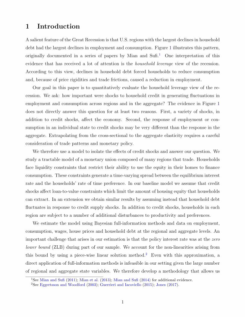
A salient feature of the Great Recession is that U.S. regions with the largest declines in household
debt had the largest declines in employment and consumption. Figure 1 illustrates this pattern,
originally documented in a series of papers by Mian and Sufi.1 One interpretation of this
evidence that has received a lot of attention is the household leverage view of the recession.
According to this view, declines in household debt forced households to reduce consumption
and, because of price rigidities and trade frictions, caused a reduction in employment.
Our goal in this paper is to quantitatively evaluate the household leverage view of the re-
cession. We ask: how important were shocks to household credit in generating fluctuations in
employment and consumption across regions and in the aggregate? The evidence in Figure 1
does not directly answer this question for at least two reasons. First, a variety of shocks, in
addition to credit shocks, affect the economy. Second, the response of employment or con-
sumption in an individual state to credit shocks may be very different than the response in the
aggregate. Extrapolating from the cross-sectional to the aggregate elasticity requires a careful
consideration of trade patterns and monetary policy.
We therefore use a model to isolate the effects of credit shocks and answer our question. We
study a tractable model of a monetary union composed of many regions that trade. Households
face liquidity constraints that restrict their ability to use the equity in their homes to finance
consumption. These constraints generate a time-varying spread between the equilibrium interest
rate and the households’ rate of time preference. In our baseline model we assume that credit
shocks affect loan-to-value constraints which limit the amount of housing equity that households
can extract. In an extension we obtain similar results by assuming instead that household debt
fluctuates in response to credit supply shocks. In addition to credit shocks, households in each
region are subject to a number of additional disturbances to productivity and preferences.
We estimate the model using Bayesian full-information methods and data on employment,
consumption, wages, house prices and household debt at the regional and aggregate levels. An
important challenge that arises in our estimation is that the policy interest rate was at the zero
lower bound (ZLB) during part of our sample. We account for the non-linearities arising from
this bound by using a piece-wise linear solution method.2 Even with this approximation, a
direct application of full-information methods is infeasible in our setting given the large number
of regional and aggregate state variables. We therefore develop a methodology that allows us
1See Mian and Sufi (2011); Mian et al. (2013); Mian and Sufi (2014) for additional evidence.2See Eggertsson and Woodford (2003); Guerrieri and Iacoviello (2015); Jones (2017).
to combine regional and aggregate data to evaluate the likelihood function.
A popular approach to modeling household debt is to assume heterogeneity in agents’ rate
of time preference, as in Iacoviello (2005) and a large literature that follows.3 These models
feature a single financial asset, which impatient households use to borrow from patient house-
holds. A tightening of credit limits reduces the amount that impatient households borrow and
translates into a one-for-one drop in their consumption, but, in the absence of changes in the
equilibrium interest rate, leaves patient households unaffected. Such models thus predict that
consumption in an individual region changes one-for-one with changes in household debt, re-
gardless of how many agents are impatient, as long as the region is sufficiently small that it does
not affect the economy-wide interest rate. One-asset models therefore imply counterfactually
large comovements between consumption and credit across regions, at odds with the evidence
in Figure 1.
Motivated by this observation, we pursue an alternative approach. We assume that house-
holds are subject to idiosyncratic shocks to their liquidity needs which make it optimal for
them to simultaneously hold liquid assets and borrow. A household can therefore respond to a
3See Eggertsson and Krugman (2012); Justiniano et al. (2015); Guerrieri and Iacoviello (2017) for the U.S.,and Martin and Philippon (2014); Gourinchas et al. (2016) for the Eurozone.
2
tightening of credit by drawing on its liquid assets instead of cutting consumption. The extent
to which it does so depends on the volatility of idiosyncratic shocks. If these shocks are volatile,
liquid assets are valuable and the household maintains its liquid asset position, thus reducing
consumption sharply after a credit tightening. If, in contrast, the volatility of idiosyncratic
shocks is low, households find it optimal to dip into their liquid assets to insulate consumption
from credit shocks. Our model thus flexibly nests both one-asset models in which a region-
specific tightening of credit leads to a large drop in consumption, as well as the frictionless
model in which credit shocks have no effect on consumption. We view this framework as our
main theoretical contribution: it is flexible enough to capture complex credit dynamics but
simple enough to be estimated on a full panel of regional economic data.
We next explain why households in our model value liquidity. The typical approach to
modeling the notion that housing equity is illiquid is to assume that agents must pay a fixed
cost to refinance their mortgage, as in the work of Kaplan et al. (2020) and Boar et al. (2020).
Since most homeowners who do not refinance are constrained,4 they save in a liquid asset in
order to smooth consumption. By contrast, considerations of computational tractability lead us
to follow an alternative approach inspired by Lucas (1990). Agents in our model can costlessly
rebalance their portfolios between periods, but they must do so prior to the realization of
an idiosyncratic preference shock. We achieve tractability by assuming a family construct to
eliminate the distributional consequences of asset market incompleteness.5 These assumptions
allow us to parsimoniously model an interest-elastic supply of liquid assets of the type that
would arise in richer but less tractable models of mortgage refinancing. In particular, the larger
the interest rate is relative to the rate of time preference, the more households save in their
liquid accounts to smooth the impact of idiosyncratic shocks. Our notion of liquidity therefore
closely resembles that in the work of Shi (2015), Rocheteau et al. (2018) and Kiyotaki and
Moore (2019) in which liquidity is valued because of idiosyncratic investment opportunity or
preference shocks.
Consider now the macroeconomic implications of a credit shock. At the economy-wide
level, a tightening of credit leads to a reduction in the natural interest rate. The drop in the
natural rate depends on the volatility of idiosyncratic preference shocks: more volatile shocks
reduce the elasticity of liquid assets and imply a larger fall in the natural rate. If prices are
sticky and monetary policy is unable to track movements in the natural rate, the credit shock
4See Amromin et al. (2007) and Adelman et al. (2010) for evidence on this.5See also Lucas and Stokey (2011) who emphasize the role of liquidity frictions and Challe and Ragot (2016)
who use a family construct to characterize an economy with uninsurable unemployment risk.
3
leads to a decline in employment. The response to economy-wide credit shocks is therefore
highly non-linear depending on how long the ZLB is expected to constrain monetary policy.
At the regional level, a tightening of credit acts like a sudden stop by forcing an increase in
the net foreign asset position, as in Gourinchas et al. (2016), but the extent of the increase
in net foreign assets depends, once again, on the volatility of idiosyncratic shocks. Hence, the
same parameter governing the elasticity of liquid assets determines both the economy-wide and
regional implications of a tightening of credit, a feature that we exploit in estimation.
We estimate three structural parameters that play a key role in shaping the economy’s re-
sponse to a credit shock: the degrees of wage and price stickiness, and the degree of idiosyncratic
uncertainty. We also estimate the persistence and volatility of the regional and aggregate shock
processes. To make full-information estimation feasible we exploit the structure of the model
and express regional level variables as deviations from the corresponding aggregates. Up to a
first-order approximation, these deviations evolve according to a law of motion that is inde-
pendent of monetary policy. This structure allows us to separate the likelihood function into
independent state-level and aggregate components. Intuitively, our estimation exploits the dif-
ferential rise and fall of individual states’ spending, employment, debt, wages and house prices,
in addition to the aggregate comovement of these series, to identify the structural parameters.
We use the model to generate counterfactual series for employment and consumption by
turning off all shocks other than credit shocks. We find that credit shocks alone account for 40
– 50% of the relative movements in state-level employment and consumption during the 2002
to 2010 period. Our findings are thus consistent with those of Mian and Sufi (2011, 2014) who
argue that household credit played an important role at the regional level.
We next discuss the model’s economy-wide implications. We distinguish between two pe-
riods: the onset of the Great Recession from 2007 to 2010, and the recovery period up to the
end of 2012. Given the non-linear nature of the responses at the ZLB, we provide bounds on
the impact of credit shocks. The lower bound assumes no ZLB. The upper bound assumes that
the ZLB binds and that the Fed does not pursue forward guidance. Under both bounds we find
that household credit shocks have a relatively small impact on employment between 2007 and
2010. In the data, employment fell by 7% during this period. In contrast, the lower and upper
bounds on the contribution of credit shocks to the decline in employment are 0.5% and 1.7%,
respectively. Thus, even under the stark assumption that the Fed did not react to credit shocks
at all, household deleveraging explains at most a quarter of the drop in employment during
the acute phase of the crisis. This result reflects the gradual nature of household deleveraging
4
which leads to a gradual decline in the natural rate.
The results are different when we consider the period 2007 to 2012. Since household debt fell
more over this longer period, so did the natural rate, and the model predicts a more important
role for credit shocks. In the data, employment was 6.2% lower by the end of 2012 compared to
2007. Under the two bounds, employment declined by 1.3% and 4.8%, respectively. The model
therefore predicts that credit shocks greatly delayed the recovery.6 Our results are robust
to a number of perturbations, including adding a construction sector, allowing for fiscal policy,
lowering the duration of mortgage contracts, explicitly modeling mortgage default, credit supply
shocks and heterogeneity in state responses to credit shocks.
Our goal in this paper is to quantify the role of credit shocks in accounting for regional
and aggregate employment during the Great Recession. To keep our analysis as transparent
as possible, we focus on the household leverage view of the Great Recession and we do not
model explicitly the other forces that arguably played an important role, such as bank and
firm-level financing constraints, changes in uncertainty, demographics, increase in markups and
risk premia. These factors are instead captured by our rich set of exogenous shocks. A limitation
of our approach is that household credit may interact with a number of these forces in important
ways.7
Related Work. Our paper is related to Eggertsson and Krugman (2012) and Guerrieri and
Lorenzoni (2017) who also study the responses of an economy to a household credit crunch.
While they study a closed-economy setting, our model is that of a monetary union composed of
a large number of regions. Moreover, our focus is on estimating the model using state-level and
aggregate data. Since we found that one-asset models cannot account for the comovement be-
tween state-level consumption and household debt, we explicitly introduce liquidity constraints
which make it optimal for households to simultaneously borrow and save in the liquid asset, an
ingredient which we argue is critical to match the regional data.
Our use of regional data to estimate the model is related to the work of Beraja et al. (2019).
These researchers apply a limited-information approach (GMM) to estimate the degree of wage
stickiness using state-level data, and then use those estimates as a prior in a full-information
estimation with only aggregate data. In contrast, we develop a methodology that allows one to
simultaneously use regional and aggregate data in a full-information approach, despite the large
6See the literature on the slow recovery discussed by Fernald et al. (2017).7For example, a tightening of household credit that depresses income and home prices may trigger a wave of
default that reduces the net worth of financial intermediaries. See Faria-e-Castro (2018) for such a model.
5
number of state variables and non-linearities associated with the ZLB. This methodology can be
fruitfully applied to other applications. Our emphasis on cross-sectional evidence is also shared
by the work of Nakamura and Steinsson (2014). Finally, our work is related to the literature
on financial intermediation, originating with Bernanke and Gertler (1989); Kiyotaki and Moore
(1997); Bernanke et al. (1999) and more recently Mendoza (2010); Gertler and Karadi (2011);
Gilchrist and Zakrajsek (2012).8
2 Model
We first describe the model economy. The economy consists of a continuum of ex-ante identical
islands of unit mass that belong to a monetary union and trade among themselves. Consumers
derive utility from a final good, leisure and housing. The final good is assembled using as
inputs traded and non-traded goods. We assume that producers of intermediate goods are
monopolistically competitive. Prices and wages are subject to Calvo adjustment frictions. Labor
is immobile across islands and the housing stock on each island is in fixed supply.
We explicitly model the distinction between liquid and illiquid assets on households’ balance
sheets. In contrast to Kaplan and Violante (2014) and much of the segmented asset markets
literature which assumes fixed costs of portfolio rebalancing, we follow instead an alternative
approach due to Lucas (1990). We assume that consumers allocate their wealth between liquid
and illiquid assets prior to the realization of an idiosyncratic preference shock. The more volatile
this shock is, the stronger the precautionary savings motive in liquid assets, and the larger the
response of consumption to credit shocks. Following Lucas (1990), we assume that consumers
belong to families that share idiosyncratic risks.
Households face shocks to their ability to tap home equity, which we refer to as credit
shocks. We also allow for shocks to the households’ rate of time preference, disutility from
work, preference for housing and productivity. Each shock has an island-specific and aggregate
component. We also assume aggregate shocks to the interest rate rule and to the aggregate
inflation equation. These additional shocks allow us to capture other channels that can explain
movements in macroeconomic aggregates.
8See also the work Lustig and Van Nieuwerburgh (2005); Garriga et al. (2019); Favilukis et al. (2017); Burnsideet al. (2016); Landvoigt et al. (2015) who study the determinants of house prices.
6
2.1 Households
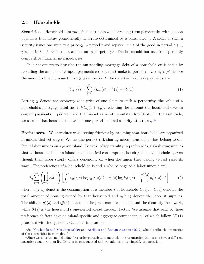
Securities. Households borrow using mortgages which are long-term perpetuities with coupon
payments that decay geometrically at a rate determined by a parameter γ. A seller of such a
security issues one unit at a price qt in period t and repays 1 unit of the good in period t + 1,
γ units in t + 2, γ2 in t + 3 and so on in perpetuity.9 The household borrows from perfectly
competitive financial intermediaries.
It is convenient to describe the outstanding mortgage debt of a household on island s by
recording the amount of coupon payments bt(s) it must make in period t. Letting lt(s) denote
the amount of newly issued mortgages in period t, the date t+ 1 coupon payments are
bt+1(s) =∞∑i=0
γilt−i(s) = lt(s) + γbt(s). (1)
Letting qt denote the economy-wide price of one claim to such a perpetuity, the value of a
household’s mortgage liabilities is bt(s)(1 + γqt), reflecting the amount the household owes in
coupon payments in period t and the market value of its outstanding debt. On the asset side,
we assume that households save in a one-period nominal security at a rate it.10
Preferences. We introduce wage-setting frictions by assuming that households are organized
in unions that set wages. We assume perfect risk-sharing across households that belong to dif-
ferent labor unions on a given island. Because of separability in preferences, risk-sharing implies
that all households on an island make identical consumption, housing and savings choices, even
though their labor supply differs depending on when the union they belong to last reset its
wage. The preferences of a household on island s who belongs to a labor union ι are
E0
∞∑t=0
(t−1∏τ=0
βτ (s)
)[∫ 1
0
vit(ι, s) log cit(ι, s)di+ ηht (s) log ht(ι, s)−ηnt (s)
1 + νnt(ι, s)
1+ν
], (2)
where cit(ι, s) denotes the consumption of a member i of household (ι, s), ht(ι, s) denotes the
total amount of housing owned by that household and nt(ι, s) denote the labor it supplies.
The shifters ηht (s) and ηnt (s) determine the preference for housing and the disutility from work,
while βt(s) is the household’s one-period ahead discount factor. We assume that each of these
preference shifters have an island-specific and aggregate component, all of which follow AR(1)
processes with independent Gaussian innovations.
9See Hatchondo and Martinez (2009) and Arellano and Ramanarayanan (2012) who describe the propertiesof these securities in more detail.
10Since we solve the model using first-order perturbation methods, the assumption that assets have a differentmaturity structure than liabilities is inconsequential and we only use it to simplify the notation.
7
The term vit(ι, s) ≥ 1 is specific to each consumer i and denotes an idiosyncratic taste shifter,
which is an i.i.d random variable drawn from a Pareto distribution over [1,∞)
Pr(vit ≤ v) = F (v) = 1− v−α. (3)
The parameter α > 1 determines the amount of uncertainty about v. A lower α implies more
uncertainty. From now on we drop the dependence on ι for notational simplicity.
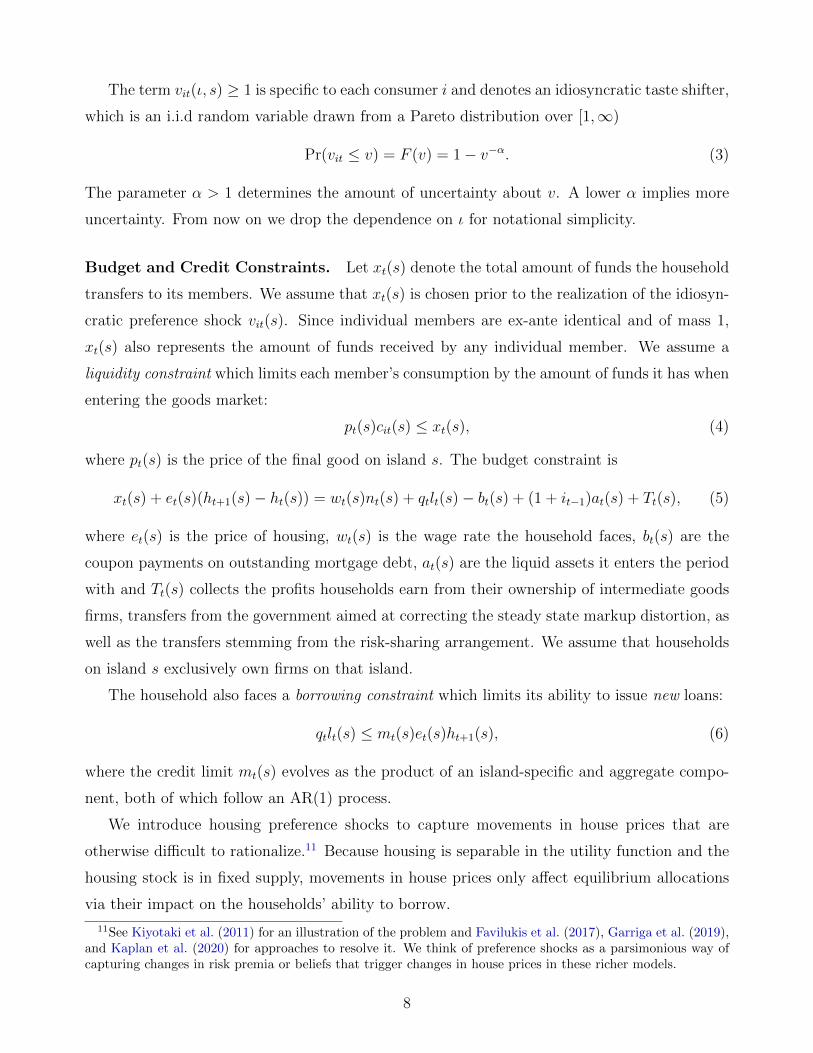
Budget and Credit Constraints. Let xt(s) denote the total amount of funds the household
transfers to its members. We assume that xt(s) is chosen prior to the realization of the idiosyn-
cratic preference shock vit(s). Since individual members are ex-ante identical and of mass 1,
xt(s) also represents the amount of funds received by any individual member. We assume a
liquidity constraint which limits each member’s consumption by the amount of funds it has when
entering the goods market:
pt(s)cit(s) ≤ xt(s), (4)
where pt(s) is the price of the final good on island s. The budget constraint is
where et(s) is the price of housing, wt(s) is the wage rate the household faces, bt(s) are the
coupon payments on outstanding mortgage debt, at(s) are the liquid assets it enters the period
with and Tt(s) collects the profits households earn from their ownership of intermediate goods
firms, transfers from the government aimed at correcting the steady state markup distortion, as
well as the transfers stemming from the risk-sharing arrangement. We assume that households
on island s exclusively own firms on that island.
The household also faces a borrowing constraint which limits its ability to issue new loans:
qtlt(s) ≤ mt(s)et(s)ht+1(s), (6)
where the credit limit mt(s) evolves as the product of an island-specific and aggregate compo-
nent, both of which follow an AR(1) process.
We introduce housing preference shocks to capture movements in house prices that are
otherwise difficult to rationalize.11 Because housing is separable in the utility function and the
housing stock is in fixed supply, movements in house prices only affect equilibrium allocations
via their impact on the households’ ability to borrow.
11See Kiyotaki et al. (2011) for an illustration of the problem and Favilukis et al. (2017), Garriga et al. (2019),and Kaplan et al. (2020) for approaches to resolve it. We think of preference shocks as a parsimonious way ofcapturing changes in risk premia or beliefs that trigger changes in house prices in these richer models.
8
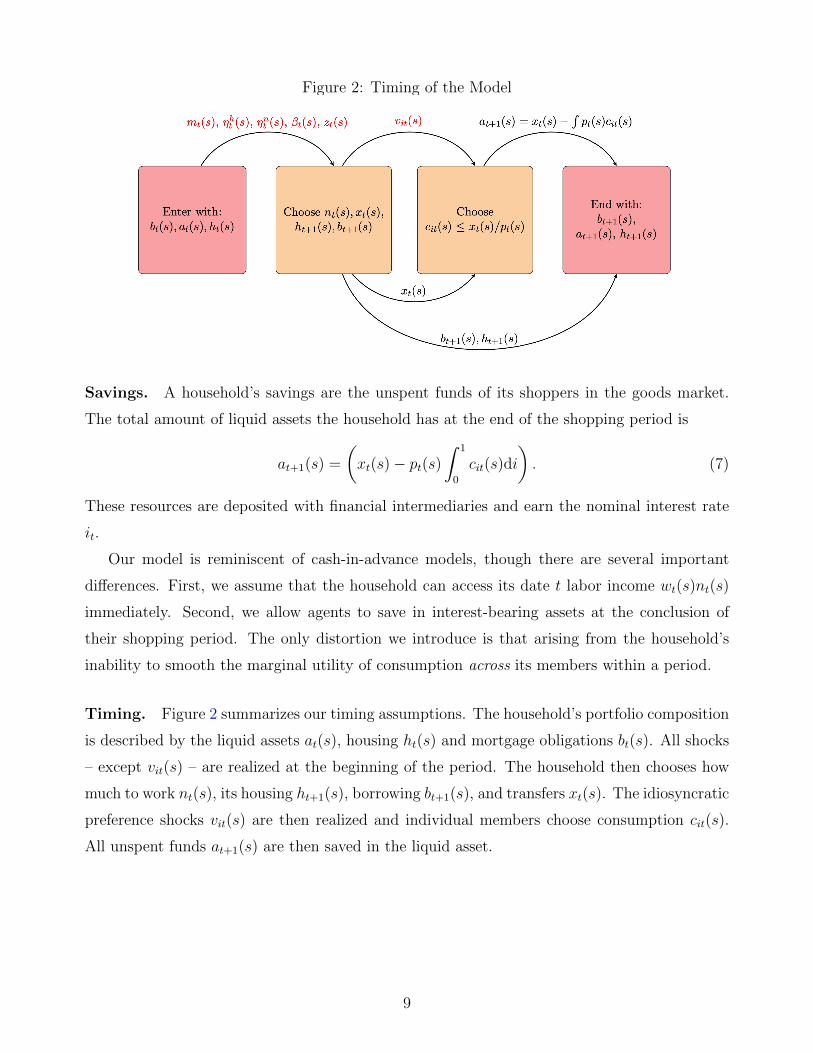
Figure 2: Timing of the Model
Savings. A household’s savings are the unspent funds of its shoppers in the goods market.
The total amount of liquid assets the household has at the end of the shopping period is
at+1(s) =
(xt(s)− pt(s)
∫ 1
0
cit(s)di
). (7)
These resources are deposited with financial intermediaries and earn the nominal interest rate
it.
Our model is reminiscent of cash-in-advance models, though there are several important
differences. First, we assume that the household can access its date t labor income wt(s)nt(s)
immediately. Second, we allow agents to save in interest-bearing assets at the conclusion of
their shopping period. The only distortion we introduce is that arising from the household’s
inability to smooth the marginal utility of consumption across its members within a period.
The left hand side is the user cost of housing. The right hand side adds the marginal utility of
housing services to the collateral value of housing.
2.4 Technology
We next discuss the assumptions we make on the technology with which final and intermediate
goods are produced.
Final Goods Producers. Final goods producers on island s produce yt(s) units of the final
good using yNt (s) units of non-tradable goods produced locally and yMt (s) units of imported
goods. Imported and non-tradable goods are combined using a CES aggregator with elasticity
of substitution σ,
yt(s) =(ω
1σ yNt (s)
σ−1σ + (1− ω)
1σ yMt (s)
σ−1σ
) σσ−1
, (18)
where ω determines the share of non-traded goods. The imported good is a CES composite of
imports from all islands with elasticity of substitution κ:
yMt (s) =
(∫ 1
0
yMt (s, s′)κ−1κ ds′
) κκ−1
. (19)
11
We assume that there are no trade costs, so all islands face the same import price index
pTt =
(∫ 1
0
pTt (s′)1−κds′) 1
1−κ
,
where pTt (s) is the price of imports from island s. Letting pNt (s) denote the price of non-tradable
goods, the final goods price on an island is
pt(s) =(ωpNt (s)1−σ + (1− ω)
(pTt)1−σ
) 11−σ
. (20)
The demand for non-tradable goods produced on an island is
yNt (s) = ω
(pNt (s)
pt(s)
)−σyt(s), (21)
while demand for its exports is the sum of purchases from all islands:
yXt (s) = (1− ω)
(pTt (s)
pTt
)−κ(∫ 1
0
(pTtpt(s′)
)−σyt(s
′)ds′
). (22)
Intermediate Goods Producers. Tradable and non-tradable goods are themselves CES
composites of varieties of differentiated intermediate inputs with an elasticity of substitution ϑ.
Technology is linear in labor and subject to a productivity disturbance zt(s) that is common to
both the tradable and non-tradable sectors:
yjkt(s) = zt(s)njkt(s), for j ∈ {X,N} .
Producers of intermediate goods are subject to Calvo pricing frictions and can only reset prices
with probability 1−θp each period. A firm that resets its price maximizes the present discounted
flow of profits weighted by the probability that the price it chooses at t will still be in effect at
any particular date. The government levies a production subsidy τp = ϑ−1ϑ
which eliminates the
steady state markup distortion and is financed with lump-sum taxes.
Wage Setting. Individual households are organized in unions that supply differentiated vari-
eties of labor with elasticity of substitution ψ. Unions reset their wages with probability 1− θweach period. We assume that the government offsets the steady-state wage markup distortion
using a subsidy τw = ψ−1ψ
financed with lump-sum transfers.
12
2.5 Monetary Policy
Let yt =∫ 1
0pt(s)yt(s)/pt ds be total output in this economy, pt =
∫ 1
0pt(s)ds be the aggregate
price level and πt = pt/pt−1 denote the rate of inflation. Aggregating the prices of individual
producers in all islands implies, up to a first-order approximation,
log(πt/π) = βEt log(πt+1/π) +(1− θp)(1− θpβ)
θp(log(wt)− log(zt)) + ηπt ,
where wt =∫wt(s)ds is the average wage in the economy, ηπt is an AR(1) disturbance to
individual firms’ desired markups, common to all islands, β is the steady state discount factor
and π is the steady-state rate of inflation.12
We follow Smets and Wouters (2007) and assume that monetary policy follows a Taylor rule
when the ZLB does not bind:
1 + it = (1 + it−1)αr[(1 + ı) (πt/π)απ y
αyt
]1−αr(yt/yt−1)αx ηit,
where ι is the steady state nominal interest rate, ηit is an i.i.d. monetary policy shock, αr
determines the persistence and απ, αy and αx determine the extent to which monetary policy
responds to deviations of inflation from the target π, the output gap yt, and the growth rate of
the output gap, respectively. The output gap is the ratio of actual output to its flexible price
level, yt = yt/y∗t . When the ZLB binds, the Fed sets it = 0.
The Fed may set an interest rate of zero not only when the ZLB binds, but also when it
follows its forward guidance. In particular, we assume that in periods in which the ZLB binds
the Fed can commit to keeping it at zero for longer than the duration prescribed by the Taylor
rule. We thus implicitly assume that the Fed can manipulate expectations of how the path of
interest rates evolves when the economy hits the ZLB, as in Eggertsson and Woodford (2003)
and Werning (2011). In our estimation we use survey data from the New York Federal Reserve
to discipline the expected duration of the zero interest rate regime between 2009 and 2015.
2.6 Asset Market
The monetary union is closed so savings in the liquid asset equal aggregate mortgage debt:∫ 1
0
at+1(s)ds =
∫ 1
0
bt+1(s)ds. (23)
12We assume in our quantitative analysis that π is equal to 2% per year. We implicitly eliminate the steady-state costs of positive inflation by assuming that all prices and wages are automatically indexed to π. See Coibionand Gorodnichenko (2015) and Blanco (2019) who study the size of these costs in the absence of indexation.
13
In contrast, individual states can run current account imbalances. An island’s net foreign asset
position evolves over time according to
at+1(s)− qtbt+1(s) = (1 + it−1)at(s)− (1 + γqt)bt(s) + pTt (s)yXt (s)− pTt yMt (s).
Perfectly competitive risk-neutral financial intermediaries borrow liquid assets from house-
holds and lend in the mortgage market. Perfect competition implies that the expected return
to holding mortgages is equal to the interest rate on the liquid asset:
EtRt+1 = 1 + it.
We next discuss the role of liquidity constraints in determining the equilibrium interest
rate in the steady state of the model. Recall that the household’s liquid savings are given
by (14). In steady state the wedge between the discount rate and the interest rate is equal to
∆ = 1β/1+i
π−1 ≈ ρ−r, where ρ = 1/β−1 is the discount rate and r = 1+i
π−1 is the real interest
rate. The upward-sloping curves in Figure 3 illustrate the households’ optimal savings choices
as a function of the real interest rate. The two panels of the Figure correspond to two scenarios,
one with a relatively high idiosyncratic uncertainty (low α), and another with a relatively low
uncertainty (high α).
To derive the demand for assets, we note that the borrowing limit binds at all times. This is
because taste shocks are unbounded, which implies that the multiplier on the liquidity constraint
ξit(s) is positive for a positive mass of household members. A comparison of (8) and (16),
together with the no-arbitrage condition EtRt+1 = 1 + it, implies that the multiplier on the
borrowing constraint µt(s) is also positive. Intuitively, since the household anticipates that a
fraction of its members will end up liquidity constrained, and since the expected return on the
mortgage is equal to the liquid interest rate, it borrows as much as possible. The result that all
households are constrained, though stark, is consistent with Boar et al. (2020) who find that
four-fifths of homeowners are constrained.
Since the credit limit binds, mortgage debt is proportional to the value of houses,
qb =m
1− γeh =
m
1− γηh
λ
1(1− m
1−βγ
)ρ+ m
1−βγ r, (24)
where the last equation follows from the Euler equation for housing (17). The value of housing
is given by the marginal utility of housing, ηh/λ, discounted by a weighted average of the rate
of time preference ρ and the interest rate r, with a weight that depends on how much the
household can borrow. As long as ρ > r, an increase in the loan-to-value ratio m reduces the
effective discount rate, raising house prices.
14
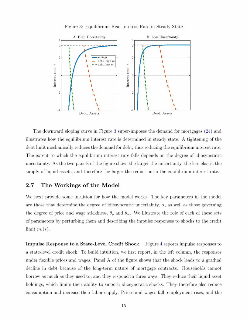
Figure 3: Equilibrium Real Interest Rate in Steady State
The downward sloping curve in Figure 3 super-imposes the demand for mortgages (24) and
illustrates how the equilibrium interest rate is determined in steady state. A tightening of the
debt limit mechanically reduces the demand for debt, thus reducing the equilibrium interest rate.
The extent to which the equilibrium interest rate falls depends on the degree of idiosyncratic
uncertainty. As the two panels of the figure show, the larger the uncertainty, the less elastic the
supply of liquid assets, and therefore the larger the reduction in the equilibrium interest rate.
2.7 The Workings of the Model
We next provide some intuition for how the model works. The key parameters in the model
are those that determine the degree of idiosyncratic uncertainty, α, as well as those governing
the degree of price and wage stickiness, θp and θw. We illustrate the role of each of these sets
of parameters by perturbing them and describing the impulse responses to shocks to the credit
limit mt(s).
Impulse Response to a State-Level Credit Shock. Figure 4 reports impulse responses to
a state-level credit shock. To build intuition, we first report, in the left column, the responses
under flexible prices and wages. Panel A of the figure shows that the shock leads to a gradual
decline in debt because of the long-term nature of mortgage contracts. Households cannot
borrow as much as they used to, and they respond in three ways. They reduce their liquid asset
holdings, which limits their ability to smooth idiosyncratic shocks. They therefore also reduce
consumption and increase their labor supply. Prices and wages fall, employment rises, and the
15
island runs a current account surplus.
The middle column of Figure 4 illustrates how price rigidities affect the response of an island
to a credit shock. We refer to this parameterization as the “Baseline” because it relies on the
parameters from our estimation below. The main impact of wage and price rigidities is to reverse
the response of employment. Price stickiness limits the increase in exports so the increase in
the current account takes place via a compression of domestic demand. The fall in employment
reduces income and consumption further. Wage rigidities act as a tax on labor supply, while
price rigidities increase firms’ markups, and both effects reduce employment.13
The last column of Figure 4 illustrates how liquidity constraints and liquidity demand affect
the response of an island to a credit shock. We reduce the volatility of idiosyncratic shocks
by increasing the parameter α. With less need to smooth large liquidity risks, households are
more willing to reduce their liquid asset holdings in response to a tightening of their borrowing
limit. As a result, consumption barely needs to fall and the impact on employment and wages
is small. These effects are capture in equation (14) which shows that liquid asset holdings
are more sensitive to the wedge between the discount rate and the interest rate when α is
high. The discount rate λt(s)βt(s)Etλt+1(s)
increases in response to the credit tightening, while the
interest rate is constant since the island is atomistic. When idiosyncratic uncertainty is low,
it is relatively costless to reduce liquid asset holdings. Both sides of the household’s balance
sheet thus contract, with little impact on other variables. In this case credit is a veil with
little impact on macroeconomic aggregates. In contrast, when idiosyncratic uncertainty is high,
reducing liquid assets is costly. Households therefore find it optimal to respond to the credit
tightening by cutting consumption.
A tightening of debt constraints thus distorts allocations in two ways: it prevents households
from smoothing the marginal utility of consumption both across members as well as across time.
Households face a tradeoff: they can respond to a tightening of credit by either reducing overall
consumption, distorting the intertemporal allocations, or by reducing liquid assets, distorting
the intrafamily allocations. The more dispersed idiosyncratic shocks are, the more the household
reduces the overall level of consumption to limit variation in the marginal utility of consumption
across its members.
Impulse Response to an Aggregate Credit Shock. To understand the effect of an ag-
gregate credit shock, we note first that the shadow value of wealth λt is approximately inversely
13See Kehoe et al. (2016) for cross-sectional evidence from the U.S. Great Recession that both of these marginsaccount for the drop in employment in states that have experience the largest declines in household credit.
16
Figure 4: Impulse Response to State-Level Credit Shock
17
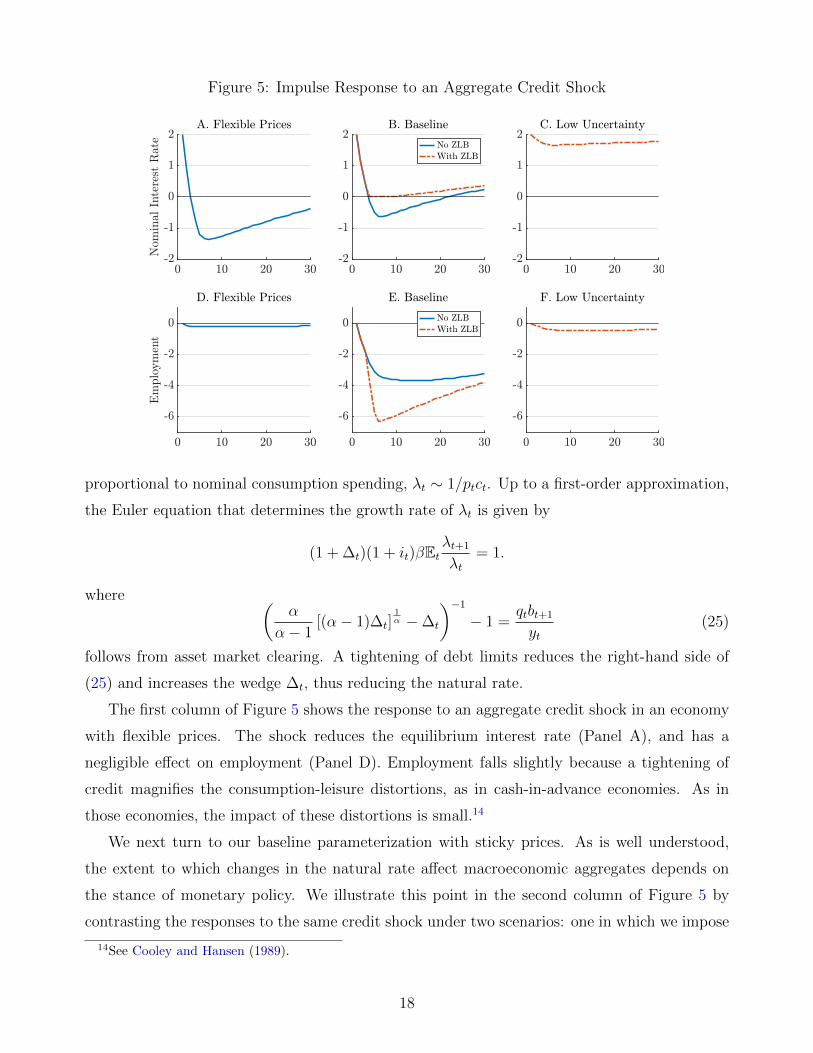
Figure 5: Impulse Response to an Aggregate Credit Shock
proportional to nominal consumption spending, λt ∼ 1/ptct. Up to a first-order approximation,
the Euler equation that determines the growth rate of λt is given by
(1 + ∆t)(1 + it)βEtλt+1
λt= 1.
where (α
α− 1[(α− 1)∆t]
1α −∆t
)−1
− 1 =qtbt+1
yt(25)
follows from asset market clearing. A tightening of debt limits reduces the right-hand side of
(25) and increases the wedge ∆t, thus reducing the natural rate.
The first column of Figure 5 shows the response to an aggregate credit shock in an economy
with flexible prices. The shock reduces the equilibrium interest rate (Panel A), and has a
negligible effect on employment (Panel D). Employment falls slightly because a tightening of
credit magnifies the consumption-leisure distortions, as in cash-in-advance economies. As in
those economies, the impact of these distortions is small.14
We next turn to our baseline parameterization with sticky prices. As is well understood,
the extent to which changes in the natural rate affect macroeconomic aggregates depends on
the stance of monetary policy. We illustrate this point in the second column of Figure 5 by
contrasting the responses to the same credit shock under two scenarios: one in which we impose
14See Cooley and Hansen (1989).
18
the ZLB and another one in which we do not. Clearly, the ZLB magnifies the reduction in
employment because it prevents the monetary authority from accommodating the decline in
the natural rate.
As in the case of island-level responses, the volatility of idiosyncratic shocks is critical in
determining how the economy reacts to a credit shock. As the last column of Figure 5 shows,
if idiosyncratic uncertainty is low, interest rates and employment fall little. In this case liquid
asset holdings are sensitive to interest rates, so a small reduction in the equilibrium rate is
required to clear the asset market. The natural rate of interest thus falls little, leading to a
negligible impact on macroeconomic outcomes.
This exercise shows that the parameters that shape the responses of island-level variables to
credit shocks also determine the aggregate-level responses. These parameters govern the slopes
of two curves: that of the Phillips curve that relates inflation to changes in marginal costs and
that of the savings curve which relates liquid asset holdings to the gap between the discount
rate and the interest rate. Since these are both functions of the primitive parameters, they
are identical in the aggregate and at the state level. In contrast, the equilibrium responses
of, say, employment to credit shocks are determined by factors such as a state’s openness to
trade and the stance of monetary policy and one cannot extrapolate state-level elasticities to
draw conclusions about the aggregate. Indeed, if monetary policy were to perfectly track the
natural rate, it would eliminate employment fluctuations in the aggregate, yet would be unable
to respond to disturbances on an individual island. We can therefore use state-level data to
identify the parameters that determine the slopes of these curves, but need to use the structure
of the model to identify the impact of credit shocks in the aggregate.
Our modeling of how households allocate their wealth between housing, liquid assets and
mortgage debt is purposefully simple and designed to capture aggregate comovements, not the
behavior of individual households. Just as the Calvo pricing protocol is a crude description
of how individual firms price, our family construct is a crude description of how individual
households save. Fully micro-founding household portfolio choices would require a rich three-
state model of the housing market similar to that studied by Kaplan et al. (2020) and Boar et
al. (2020). Such a model would entail significant micro-level non-convexities that would make
full-information estimation infeasible. Since our goal is to use state-level data to isolate the
impact of monetary policy in stabilizing the response of real variables to credit shocks, our
conjecture is that our simplification provides a useful approximation, analogous to the Calvo
pricing approach in modeling the dynamics of inflation.
19
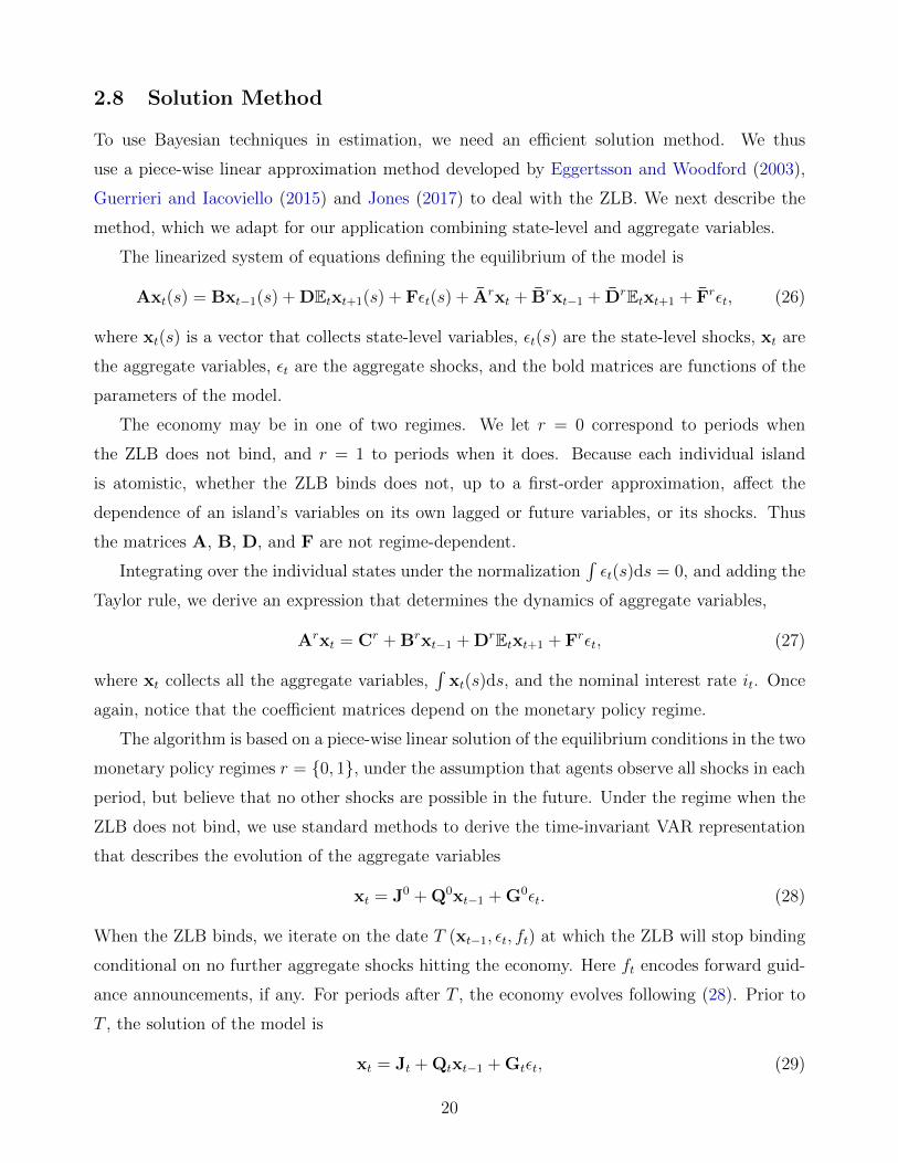
2.8 Solution Method
To use Bayesian techniques in estimation, we need an efficient solution method. We thus
use a piece-wise linear approximation method developed by Eggertsson and Woodford (2003),
Guerrieri and Iacoviello (2015) and Jones (2017) to deal with the ZLB. We next describe the
method, which we adapt for our application combining state-level and aggregate variables.
The linearized system of equations defining the equilibrium of the model is
The matrices Jt, Qt, and Gt encode how an island responds to aggregate-level variables and
vary over time because of the ZLB. In contrast, the matrices Q and G which determine how
an island’s variables depend on their own lags and island-specific shocks are time-invariant.
Intuitively, since each island is of measure zero, shocks to an individual island do not change
the expected date at which the ZLB will stop binding for the rest of the economy. Moreover,
agents on each island take aggregate prices, including the interest rate, as given. Therefore,
conditional on the aggregate state variables, the ZLB regime does not affect the evolution of
island-level relative variables. From the perspective of agents on a given island, the presence of
the ZLB acts like any other aggregate shock which, up to a first-order approximation, does not
change how that island responds to its own history of idiosyncratic shocks.
Equation (31) reveals that our model has a special structure. First, the mapping from state-
level histories of shocks to state-level outcomes is time-invariant and common to all states.
Second, the mapping from aggregate histories of shocks to state-level variables, though time-
varying, is also common to all states. We exploit this structure to construct the likelihood
function, as we describe below.
15See Kulish and Pagan (2017) and Jones (2017) for more details on the recursion underlying this solution.Jones (2017) contrasts this method with fully non-linear ones in smaller scale models and shows that that thepiece-wise linear method we use here is accurate. Lepetyuk et al. (2017) contrast these perturbation-basedmethods with fully non-linear projection methods in larger-scale models and reach similar conclusions regardingtheir accuracy.
21
3 Estimation
We next explain how we chose parameters for our model. We first discuss the parameters we
assign values to, and then the ones we estimate.
The parameters that we estimate are those that are critical in determining the model’s
responses to a credit shock: the degree of wage and price stickiness, θw and θp, as well as
the volatility of idiosyncratic taste shocks, α. We refer to these parameters as our structural
parameters. In addition, we estimate the AR(1) processes characterizing the island-specific and
aggregate components of the various shocks. We next describe the parameters we have assigned,
the construction of the likelihood function, and then our results.
3.1 Assigned Parameters
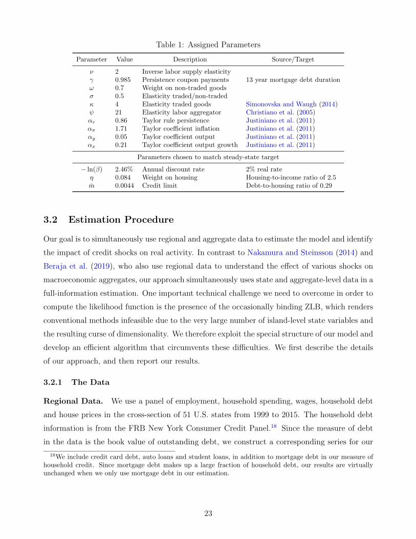
We report the parameter values we assign in Table 1. The period is one quarter. We assume
a Frisch elasticity of labor supply of 1/2. We set γ, the parameter governing the duration
of debt, to 0.985, so that the Macaulay duration of debt in our model is equal to that of
mortgage debt in the data, approximately 13 years.16 We follow the trade literature in setting
the weight on non-traded goods in an island’s consumption basket, ω, equal to 0.7; the elasticity
of substitution between tradable and non-tradable goods, σ, equal to 0.5; and the elasticity of
substitution between varieties of tradable goods produced in different islands, κ, equal to 4, the
estimate of Simonovska and Waugh (2014). We follow Christiano et al. (2005) in choosing ψ to
ensure a wage markup of 5%.17 We use the Justiniano et al. (2011) estimates of the parameters
characterizing the Taylor rule.
We pin down three additional parameters using steady state considerations. The steady
state discount factor β is chosen so that the steady state real interest rate is equal to 2% per
year. The steady state weight of housing in preferences ηh is chosen so that the aggregate
housing to (annual) income ratio is equal to 2.5, a number that we compute using the 2001
Survey of Consumer Finances (SCF). Finally, the steady state LTV ratio is chosen so that the
aggregate debt to housing ratio is equal to 0.29, a number once again computed from the SCF.
Since the debt constraint binds in the model, these two last two targets imply an aggregate
debt to (annual) income ratio of 2.5× 0.29 = 0.725.
16The Macaulay duration is the weighted average maturity of the flows, with weights given by the presentvalue of the flows accruing at each date. In our model with geometrically decaying perpetuities this duration isgiven by (1 + r)/(1 + r − γ).
17We show in our Robustness section that our conclusions are not sensitive to alternative values of ψ.
22
Table 1: Assigned Parameters
Parameter Value Description Source/Target
ν 2 Inverse labor supply elasticityγ 0.985 Persistence coupon payments 13 year mortgage debt durationω 0.7 Weight on non-traded goodsσ 0.5 Elasticity traded/non-tradedκ 4 Elasticity traded goods Simonovska and Waugh (2014)ψ 21 Elasticity labor aggregator Christiano et al. (2005)αr 0.86 Taylor rule persistence Justiniano et al. (2011)απ 1.71 Taylor coefficient inflation Justiniano et al. (2011)αy 0.05 Taylor coefficient output Justiniano et al. (2011)αx 0.21 Taylor coefficient output growth Justiniano et al. (2011)
Parameters chosen to match steady-state target
− ln(β) 2.46% Annual discount rate 2% real rateη 0.084 Weight on housing Housing-to-income ratio of 2.5m 0.0044 Credit limit Debt-to-housing ratio of 0.29
3.2 Estimation Procedure
Our goal is to simultaneously use regional and aggregate data to estimate the model and identify
the impact of credit shocks on real activity. In contrast to Nakamura and Steinsson (2014) and
Beraja et al. (2019), who also use regional data to understand the effect of various shocks on
macroeconomic aggregates, our approach simultaneously uses state and aggregate-level data in a
full-information estimation. One important technical challenge we need to overcome in order to
compute the likelihood function is the presence of the occasionally binding ZLB, which renders
conventional methods infeasible due to the very large number of island-level state variables and
the resulting curse of dimensionality. We therefore exploit the special structure of our model and
develop an efficient algorithm that circumvents these difficulties. We first describe the details
of our approach, and then report our results.
3.2.1 The Data
Regional Data. We use a panel of employment, household spending, wages, household debt
and house prices in the cross-section of 51 U.S. states from 1999 to 2015. The household debt
information is from the FRB New York Consumer Credit Panel.18 Since the measure of debt
in the data is the book value of outstanding debt, we construct a corresponding series for our
18We include credit card debt, auto loans and student loans, in addition to mortgage debt in our measure ofhousehold credit. Since mortgage debt makes up a large fraction of household debt, our results are virtuallyunchanged when we only use mortgage debt in our estimation.
23
model using
debtt(s) = γdebtt−1(s) + qtlt(s),
where qtlt(s) is the market value of mortgage debt issued in period t and γdebtt−1(s) is the
book value of outstanding debt. We found that our results are unchanged if we instead use the
market value of debt qtbt+1(s)to proxy for household credit in the data.
We use data on house prices from the FHFA, and data on employment, consumption expen-
ditures and wages from the BEA. Our measure of employment is the employment-population
ratio in a given state. Our measure of wages is total employee compensation divided by the
number of workers. Since we do not model the construction sector, we subtract construction
employment and compensation in computing measures of employment and wages.19
Aggregate Data. We use aggregate data on employment, household consumption expendi-
tures, wages, household debt, house prices, inflation and the Fed Funds rate from 1984 to 2015.
We construct this data in a similar way to the state-level data. An additional critical input in
the estimation is the sequence of expected durations of the ZLB between 2009 and 2015, which
we take from the Blue Chip Financial Forecasts survey from 2009 to 2010 and the New York
Federal Reserve’s Survey of Primary Dealers from 2011 to 2015.20
3.2.2 The Likelihood Function
The conventional approach to estimating the model would be to write down a likelihood function
that directly combines state and aggregate data. This approach is computationally infeasible
because of the non-linearity induced by the ZLB and the curse of dimensionality which arises
from our use of 51 regions, each of which has 11 individual state variables.
We thus use the structure of our model to formulate an alternative approach to constructing
the likelihood function, one that exploits relative variation across individual states’ outcomes.
Intuitively, our approach recognizes that, up to a first-order approximation, the difference be-
tween employment in, say, Nevada and in the aggregate is a linear function of the Nevada state
variables only. This observation allows us to separate the likelihood into state-level components
and an aggregate component.
To understand our approach, recall that the evolution of variables in any given state is given
19See our Robustness section for an extension that explicitly models the construction sector and uses data onconstruction employment in estimation. Our results are robust to this modification.
20See the Appendix for a more detailed description of the data we use.
24
by (31), which we reproduce here for convenience:
xt(s) = Qxt−1(s) + Gεt(s) + Jt + Qtxt−1 + Gtεt.
Since the last three reduced-form matrices are time-varying functions of the underlying struc-
tural parameters whenever the ZLB binds, computing them for each parameter draw in the
estimation is infeasible. The special structure of the model allows us, however, to write the
deviation of island-level variables from their economy-wide averages,
xt(s) = xt(s)−∫
xt(s)ds, (32)
as a time-invariant function of island-level variables alone:
xt(s) = Qxt−1(s) + Gεt(s). (33)
This structure allows us to significantly speed up the computation of the likelihood function.
We therefore use the representation in (29) and (33) to estimate the model using state-level
and aggregate U.S. data. To do so, we first express each state’s observable variable as deviations
from its aggregate counterpart by subtracting a full set of time effects, one for each year and
each variable. We also subtract a state-specific fixed effect and time trend for each observable
since in our model all islands are ex-ante identical.21 Since the island-level shocks in (33)
are independent and do not affect aggregate outcomes, we can write the log-likelihood of the
model as the sum of each individual state’s likelihood, computed from (33) and the aggregate
likelihood, computed from (29):
logL =51∑s=1
ω(s) logL(s) + logLa,
where L(s) is the contribution to the likelihood of an individual state’s data, La is the contri-
bution to the likelihood of the aggregate data, and ω(s) is the relative weight of state s. This
additive structure follows from the block exogeneity implied by our representation (33) which
allows us to express the determinant of the variance-covariance matrix of the forecast errors as
the product of the determinants of the variance-covariance matrices of the individual states.
To see how we construct the likelihood for an individual state, denote by N = 5 the number
of observable variables and T = 17 (1999 to 2015) the number of years of data that are available.
With Gaussian errors, the log-likelihood function for any individual state is
logL(s) = −(N T
2
)log 2π − 1
2
T∑t=1
log det St −1
2
T∑t=1
x′t(s)S−1t xt(s).
21In practice, subtracting the state-specific fixed effects only, as we have done in an earlier version of thepaper, does not change our substantive results.
25
where xt(s) is the vector of forecast errors, calculated using the Kalman filter and the structural
matrices Q and G from (33), and St is the covariance matrix of xt(s). We compute the aggregate
likelihood component in a similar fashion, taking into account that the sequence of forecast
errors and their covariance matrices are functions of the underlying time-varying reduced-form
matrices Qt and Gt from (29) (see the Appendix for details).
To summarize, our estimation exploits the differential rise and fall of individual states’
spending, debt, wages, house prices and employment, in addition to the aggregate comovement
of these series, to identify the structural parameters of the model. Notice that by simultaneously
using state and aggregate data to construct the likelihood, our approach differs from that of
Beraja et al. (2019). These researchers first apply limited information methods (GMM) to
estimate the degree of wage stickiness using state-level data. They then use that estimate to
form a prior in a second step, which uses only aggregate data to form the likelihood function.
The state-level data is observed at an annual frequency, while the model is quarterly, so
we conduct a mixed-frequency estimation, by computing forecast errors every four quarters for
state-level variables. The aggregate data, in contrast, is observed quarterly and for a longer time-
period, from 1984 to 2015. To account for differences in the size of different states and ensure
that smaller states exert a relatively smaller influence on the shape of the likelihood, we weight
the likelihood contribution of each state by their 1999 population shares.22 In a robustness
exercise reported below, we also compute the likelihood without weighting individual states. In
our baseline estimation, we assign an equal weight to the aggregate likelihood and the combined
state-level likelihood.
3.3 Parameter Estimates
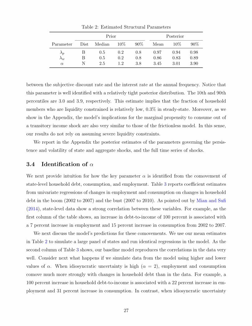
Table 2 reports moments of the prior and posterior distributions of the structural parameters
we estimate. We use diffuse priors. We find, consistent with the work of Del Negro et al. (2015),
that wages and prices are sticky, with a modal estimate of θp of 0.97 and a modal estimate of θw
of 0.86. As is well known, accounting for the stability of inflation around the Great Recession
requires a great deal of price stickiness. We show below that estimating the model using state-
level data alone implies a much lower degree of price stickiness, consistent with the evidence in
Beraja et al. (2019). We explore the implications of this alternative set of parameter estimates
in our Robustness section below.
The mean estimate of the Pareto tail parameter α is equal to 3.45, implying a 0.47% spread
22See Agostinelli and Greco (2012) who show that this simple weighting scheme preserves the asymptoticproperties of the true likelihood function.
26
Table 2: Estimated Structural Parameters
Prior Posterior
Parameter Dist Median 10% 90% Mean 10% 90%
λp B 0.5 0.2 0.8 0.97 0.94 0.98λw B 0.5 0.2 0.8 0.86 0.83 0.89α N 2.5 1.2 3.8 3.45 3.01 3.90
between the subjective discount rate and the interest rate at the annual frequency. Notice that
this parameter is well identified with a relatively tight posterior distribution. The 10th and 90th
percentiles are 3.0 and 3.9, respectively. This estimate implies that the fraction of household
members who are liquidity constrained is relatively low, 0.3% in steady-state. Moreover, as we
show in the Appendix, the model’s implications for the marginal propensity to consume out of
a transitory income shock are also very similar to those of the frictionless model. In this sense,
our results do not rely on assuming severe liquidity constraints.
We report in the Appendix the posterior estimates of the parameters governing the persis-
tence and volatility of state and aggregate shocks, and the full time series of shocks.
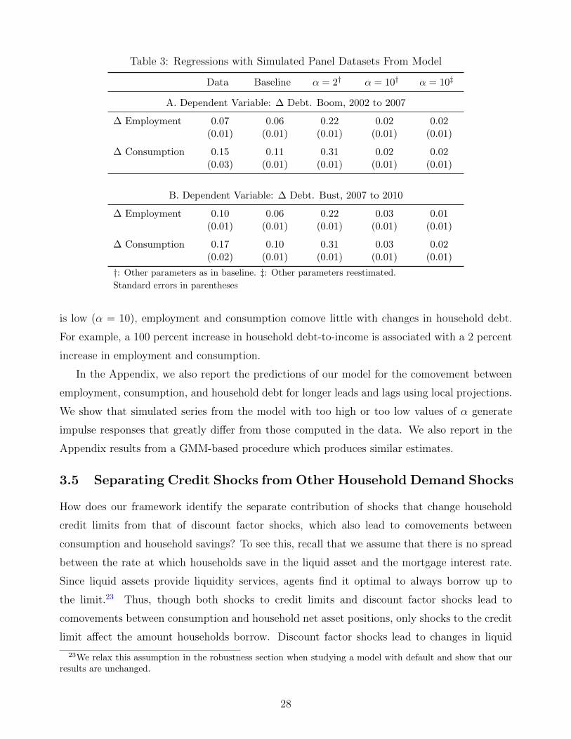
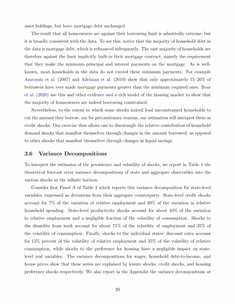
3.4 Identification of α
We next provide intuition for how the key parameter α is identified from the comovement of
∆ Employment– 2002 to 2007 0.47 0.05 −0.09 −0.09 0.58– 2007 to 2010 0.52 0.04 0.14 −0.08 0.38
∆ Consumption– 2002 to 2007 0.27 0.03 0.00 −0.08 0.74– 2007 to 2010 0.48 0.03 0.00 −0.03 0.55
these results are not simply an artefact of the modeling choices we have made, but rather a
result of the estimation and the path for shocks extracted by the Kalman smoother from the
data. If instead we used a higher value of α in simulating the model, credit shocks would have
had much smaller effects, as we report in our Robustness section.
Table 5 illustrates the role of all additional shocks in explaining the relative changes in
employment and consumption during these two periods. We use the Kalman smoother to extract
the shocks and construct counterfactual employment and consumption panels by turning on one
shock at a time. Table 5 reports the slope coefficients of the projection of the counterfactual
series on the actual data.24 In addition to the credit shocks, discount factor shocks account for
the bulk of the remaining fluctuations in employment and consumption. These shocks capture
other sources of state-level movements in consumption, such as perhaps heterogeneity in fiscal
transfers across states, expectations of future growth, precautionary savings motives, and other
factors. In our Robustness section, we show that explicitly introducing differential changes in
government spending across states reduces the contribution of discount factor shocks, but leaves
the contribution of credit shocks unchanged.
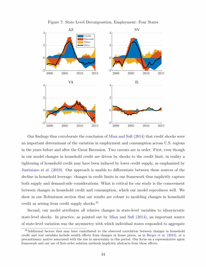
We next zoom in on several states and show in Figure 7 how the time-series of relative
employment is shaped by credit, discount factor, and other shocks. The top row of the figure
plots relative employment for two states – Arizona and Nevada – that experienced large changes
in credit and employment. The bottom row of the figure shows two contrasting states – Virginia
and Illinois – that experienced mild fluctuations. The figure reinforces the point that credit
shocks were an important driver of the relative change in employment across states over this
period. In the Appendix, we show similar decompositions for all states, along with the full time
series of shocks.
24These coefficients do not sum to one because part of the variation of the observable series is attributed toinitial conditions.
33
Figure 7: State Level Decomposition, Employment: Four States
Our findings thus corroborate the conclusion of Mian and Sufi (2014) that credit shocks were
an important determinant of the variation in employment and consumption across U.S. regions
in the years before and after the Great Recession. Two caveats are in order. First, even though
in our model changes in household credit are driven by shocks to the credit limit, in reality a
tightening of household credit may have been induced by lower credit supply, as emphasized by
Justiniano et al. (2019). Our approach is unable to differentiate between these sources of the
decline in household leverage: changes in credit limits in our framework thus implicitly capture
both supply and demand-side considerations. What is critical for our study is the comovement
between changes in household credit and consumption, which our model reproduces well. We
show in our Robustness section that our results are robust to modeling changes in household
credit as arising from credit supply shocks.25
Second, our model attributes all relative changes in state-level variables to idiosyncratic
state-level shocks. In practice, as pointed out by Mian and Sufi (2014), an important source
of state-level variation was the asymmetry with which individual states responded to aggregate
25Additional factors that may have contributed to the observed correlation between changes in householdcredit and real variables include wealth effects from changes in house prices, as in Berger et al. (2018), or aprecautionary motive associated with the rise in uncertainty in this period. Our focus on a representative agentframework and our use of first-order solution methods implicitly abstracts from these effects.
34
shocks. The approach we pursue is motivated by tractability considerations: if the matrices
Jt, Qt and Gt of equation (31) that determine how an individual island responds to aggregate
shocks were state-specific, say due to heterogeneity in housing supply elasticities, the likelihood
function would not be additively separable into individual state-level likelihood contributions.
Our estimates of the state-level shocks should therefore be interpreted more broadly as capturing
not only state-specific idiosyncratic disturbances, but also heterogeneity in the extent to which
state-level variables responded to aggregate shocks. In our Robustness section, we relax the
assumption that all states react in an identical way to state and aggregate shocks by separating
states into three groups that differ in their housing supply elasticities. In this extension we
can only use state-level data to estimate the parameters, but find that our estimates of the key
structural parameters and the model’s implications for the relative importance of credit shocks
are similar to those in the baseline.
4.2 Role of Credit Shocks at the Aggregate Level
We next turn to discussing the model’s implications for the role of credit shocks in explaining
fluctuations in the aggregate. Figure 8 presents the dynamics of the key aggregate time series
during the 1995 to 2015 period in the data. We HP-filter the debt-to-income series and report
it as deviations from the trend in Panel A. Panel B reports the evolution of the Fed Funds Rate
and the implied natural rate predicted by the model. Panel C reports the data on employment,
measured as the total number of employees on non-farm payrolls, scaled by the U.S. popula-
tion and expressed as percent deviations from a linear trend. Panel D shows the time series
for inflation. We used these series, together with aggregate data on wages, house prices and
consumption, to extract the aggregate component of the exogenous shocks used in estimation.
We construct a counterfactual series for each of these variables by shutting down all shocks
other than credit shocks. Panel A of Figure 8 shows that credit shocks drive most of the
movements in household credit. As Panel B shows, however, credit shocks alone generate
modest movements in the natural rate of interest. Specifically, our estimates imply that the
natural rate declined from 4.7% at the beginning of 2007 to -1.4% by the end of 2012. Credit
shocks account for only one-tenth of this decline: the natural rate would have fallen from 2.4%
to 1.8% in the absence of other shocks.
Consider next how employment responds to credit shocks. As the lower-left panel of Fig-
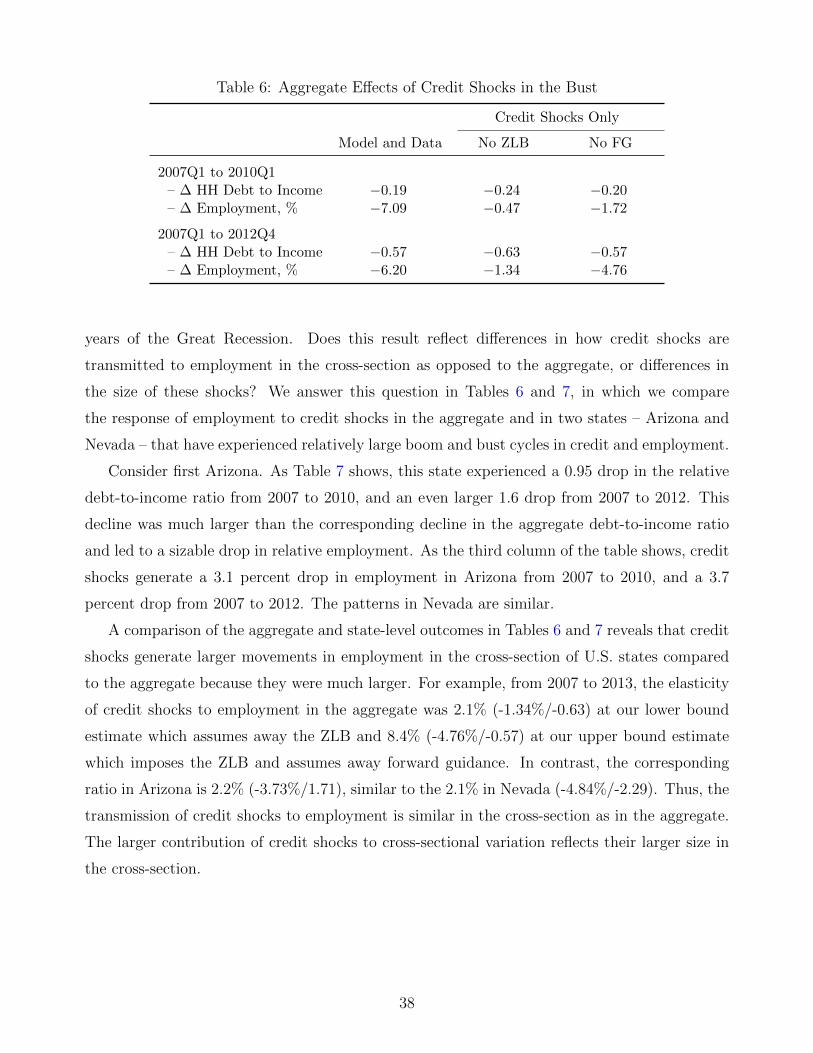
ure 8 and Table 6 shows, the Great Recession was associated with a nearly 6.2% drop in the
employment-population ratio from 2007 to 2012. Credit shocks alone account for a modest 1.3%
35
Figure 8: Effect of Credit Shocks Alone on Aggregate Variables
drop, one-fifth of the actual decline. Employment falls little because credit shocks generate a
small decline in the natural rate, insufficient to trigger the ZLB. Absent additional shocks mon-
etary policy is unconstrained and mimics the dynamics of the natural rate well, implying minor
movements in employment and inflation. As is well-understood, however, the ZLB brings about
important non-linearities in how aggregate variables respond to shocks. If household credit
shocks are accompanied, as they were in the data, by other shocks that reduce the Fed’s ability
to cut interest rates because of the ZLB, the resulting effects on output can be much greater.
How much greater?
Answering this question is challenging because of the Fed’s pursuit of forward guidance
policies. In our estimation we have taken the Fed’s forward guidance announcements as given,
by setting the expected ZLB duration each quarter equal to the expectations in the data. Since
these announcements were responding to the path of all shocks, including credit shocks, we
cannot isolate the effect of credit shocks alone without taking a stand on how forward guidance
would have been conducted absent such shocks. In short, the pursuit of forward guidance poses
an identification challenge, one of decomposing the expected ZLB durations into an endogenous
component due to shocks, and one due to forward guidance policies.26
We address this challenge by providing bounds on the role of credit shocks under two extreme
26See Jones (2017) for a more detailed discussion of this identification problem and a solution to it.
36
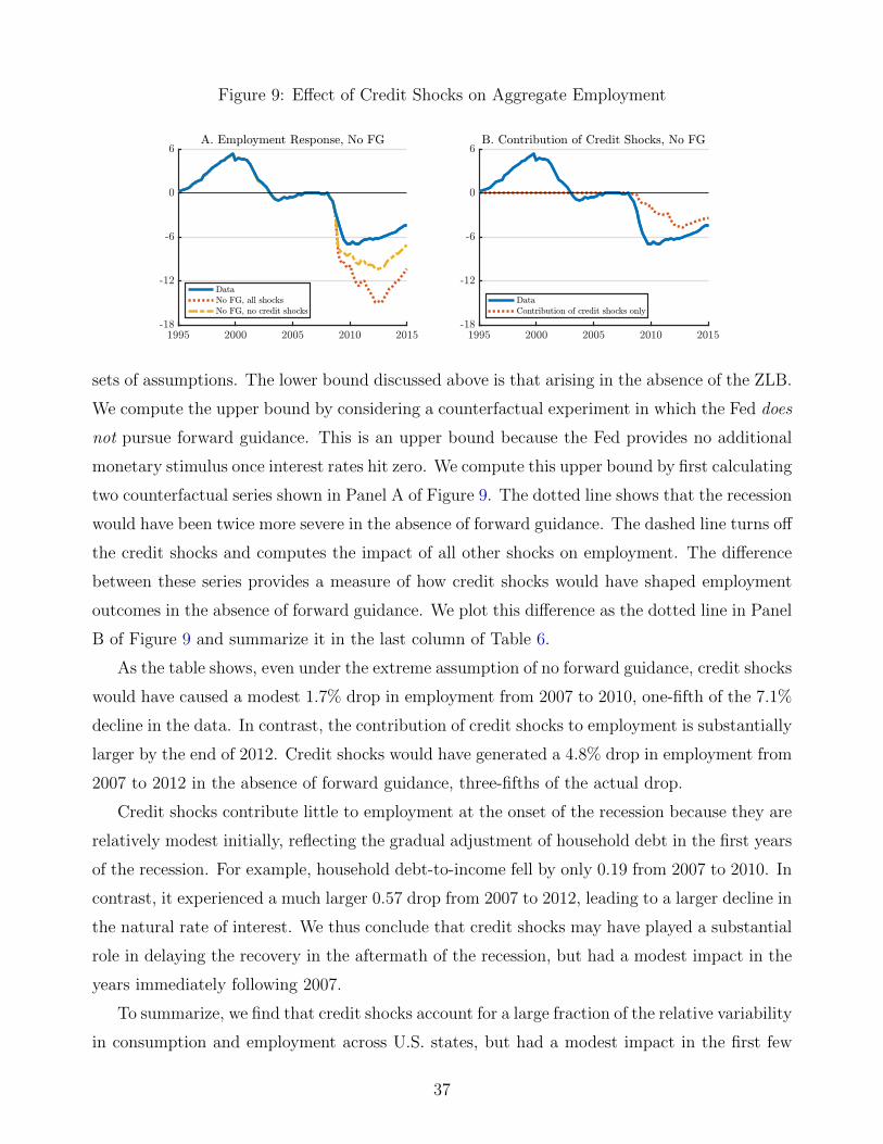
Figure 9: Effect of Credit Shocks on Aggregate Employment
sets of assumptions. The lower bound discussed above is that arising in the absence of the ZLB.
We compute the upper bound by considering a counterfactual experiment in which the Fed does
not pursue forward guidance. This is an upper bound because the Fed provides no additional
monetary stimulus once interest rates hit zero. We compute this upper bound by first calculating
two counterfactual series shown in Panel A of Figure 9. The dotted line shows that the recession
would have been twice more severe in the absence of forward guidance. The dashed line turns off
the credit shocks and computes the impact of all other shocks on employment. The difference
between these series provides a measure of how credit shocks would have shaped employment
outcomes in the absence of forward guidance. We plot this difference as the dotted line in Panel
B of Figure 9 and summarize it in the last column of Table 6.
As the table shows, even under the extreme assumption of no forward guidance, credit shocks
would have caused a modest 1.7% drop in employment from 2007 to 2010, one-fifth of the 7.1%
decline in the data. In contrast, the contribution of credit shocks to employment is substantially
larger by the end of 2012. Credit shocks would have generated a 4.8% drop in employment from
2007 to 2012 in the absence of forward guidance, three-fifths of the actual drop.
Credit shocks contribute little to employment at the onset of the recession because they are
relatively modest initially, reflecting the gradual adjustment of household debt in the first years
of the recession. For example, household debt-to-income fell by only 0.19 from 2007 to 2010. In
contrast, it experienced a much larger 0.57 drop from 2007 to 2012, leading to a larger decline in
the natural rate of interest. We thus conclude that credit shocks may have played a substantial
role in delaying the recovery in the aftermath of the recession, but had a modest impact in the
years immediately following 2007.
To summarize, we find that credit shocks account for a large fraction of the relative variability
in consumption and employment across U.S. states, but had a modest impact in the first few
37
Table 6: Aggregate Effects of Credit Shocks in the Bust
Credit Shocks Only
Model and Data No ZLB No FG
2007Q1 to 2010Q1– ∆ HH Debt to Income −0.19 −0.24 −0.20– ∆ Employment, % −7.09 −0.47 −1.72
2007Q1 to 2012Q4– ∆ HH Debt to Income −0.57 −0.63 −0.57– ∆ Employment, % −6.20 −1.34 −4.76
years of the Great Recession. Does this result reflect differences in how credit shocks are
transmitted to employment in the cross-section as opposed to the aggregate, or differences in
the size of these shocks? We answer this question in Tables 6 and 7, in which we compare
the response of employment to credit shocks in the aggregate and in two states – Arizona and
Nevada – that have experienced relatively large boom and bust cycles in credit and employment.
Consider first Arizona. As Table 7 shows, this state experienced a 0.95 drop in the relative
debt-to-income ratio from 2007 to 2010, and an even larger 1.6 drop from 2007 to 2012. This
decline was much larger than the corresponding decline in the aggregate debt-to-income ratio
and led to a sizable drop in relative employment. As the third column of the table shows, credit
shocks generate a 3.1 percent drop in employment in Arizona from 2007 to 2010, and a 3.7
percent drop from 2007 to 2012. The patterns in Nevada are similar.
A comparison of the aggregate and state-level outcomes in Tables 6 and 7 reveals that credit
shocks generate larger movements in employment in the cross-section of U.S. states compared
to the aggregate because they were much larger. For example, from 2007 to 2013, the elasticity
of credit shocks to employment in the aggregate was 2.1% (-1.34%/-0.63) at our lower bound
estimate which assumes away the ZLB and 8.4% (-4.76%/-0.57) at our upper bound estimate
which imposes the ZLB and assumes away forward guidance. In contrast, the corresponding
ratio in Arizona is 2.2% (-3.73%/1.71), similar to the 2.1% in Nevada (-4.84%/-2.29). Thus, the
transmission of credit shocks to employment is similar in the cross-section as in the aggregate.
The larger contribution of credit shocks to cross-sectional variation reflects their larger size in
the cross-section.
38
Table 7: Relative State-Level Effects of Credit Shocks in the Bust
Model and Data Credit Shocks Only
Arizona Nevada Arizona Nevada
2007 to 2010– ∆ HH Debt to Income −0.95 −1.39 −1.01 −1.46– ∆ Employment, % −3.11 −3.47 −3.13 −4.02
2007 to 2013– ∆ HH Debt to Income −1.60 −2.15 −1.71 −2.29– ∆ Employment, % −3.07 −2.41 −3.73 −4.84
5 Robustness
We conclude by considering a number of robustness checks. For brevity, here we only report the
various models’ implications for the importance of credit shocks in accounting for state-level
and aggregate movements in employment and consumption. In the Appendix we report the
parameter estimates. Table 8 reports the various models’ implications for the contribution of
state-level credit shocks to the relative changes of state-level employment and consumption.
Table 9 reports the models’ aggregate implications.
No Population Weighting. In this robustness exercise, we estimate the model’s parameters
without population-weighting the contribution of individual states to the likelihood function.
As Tables 8 and 9 show, our results are unaffected.
Remove 5 Largest States. One concern is that shocks to large states may have important
aggregate consequences, invalidating our approach of assuming independent state-level and ag-
gregate shocks. To address this concern, we examined the robustness of our results to removing
the five largest states from the estimation. Specifically, we re-estimated the model without data
on California, Texas, New York, Florida, and Illinois. As Tables 8 and 9 report, the estimated
model’s implications for the contribution of credit shocks at both the state and aggregate level
are similar to those in our baseline.
State Data Only. Here we estimate the model’s structural parameters using regional data
alone. We then fix these parameters and use the aggregate data to only estimate the parameters
of the aggregate shock processes. As we show in the Appendix, using state-level data only we
estimate a much lower degree of wage and price stickiness. Intuitively, as Beraja et al. (2019)
39
Table 8: Contribution of State Credit Shocks to State-Level Variables
High and Low Uncertainty. Here we illustrate the role played by the volatility of idiosyn-
cratic taste shocks. We first reduce the volatility of taste shocks by increasing α to 5 and
re-estimating all other parameters. As Table 8 shows, credit shocks now produce much smaller
relative movements in employment and consumption across states. When idiosyncratic un-
certainty is low, agents in a state subject to a credit tightening consume out of their liquid
assets, so consumption and employment change little. Similarly, as Table 9 shows, credit shocks
alone generate virtually no employment decline in the aggregate even at our upper bound that
assumes no forward guidance.
We next increase the volatility of taste shocks by lowering α to 2. The model now attributes a
significantly larger role to credit shocks in explaining state-level movements in real variables. As
Table 8 shows, credit shocks generate twice more volatile series for employment and consumption
during the bust compared to the data. The model also ascribes a much more important role to
credit shocks in explaining the aggregate employment decline. Even in the absence of the ZLB,
the model predicts an almost 6 percent decline in employment from 2007 to 2012.
Lower Debt Duration and One-period Debt. So far we have imposed a value of γ, the
parameter determining the decay rate of coupon payments in the mortgage contract, equal
to 0.985, consistent with the maturity of mortgage contracts in the data. One could argue,
however, that the effective duration of mortgages in the data is lower, due to households’ ability
41
to refinance their mortgages or take on home equity loans. Here we reduce γ to 0.965, implying
a duration of mortgages about half that in our baseline (6 years versus 13 years) and reestimate
the model. Table 8 shows that credit shocks now generate somewhat larger relative movements
in employment and consumption across U.S. states. Similarly, Table 9 shows that credit shocks
now account for a larger drop in aggregate employment during the recovery. For example, credit
shocks alone predict a 3.3% drop in employment from 2007 to 2012 even in the absence of the
ZLB and a 6.6% drop at the ZLB and in the absence of forward guidance.
We have also considered a version of the model with one-period debt, by setting γ = 0.
To help match the slow-moving debt and house prices, we now assume that the shocks to
credit and preference for housing are themselves AR(1) processes. As Table 8 reports, the
model’s implications for the role of credit shocks in the cross-section are very similar to those in
our Benchmark parameterization. Mechanically, the persistence and volatility of credit shocks
adjusts when we change γ so as to match the comovement of credit and real variables in the
data, with little consequence for the behavior of other variables. At the aggregate-level, as Table
9 shows, the implications of credit shocks over the 2007 to 2010 period are unchanged compared
to our baseline estimates. However, with one-period debt, credit shocks are more important
over the 2007 to 2012 period.
Lower Labor Elasticity. In our baseline estimation, we assigned a value of this elasticity, ψ,
equal to 21, following Christiano et al. (2005). This parameter acts like a real rigidity, in that it
prevents reset wages from responding too much to a given shock. Here we reduce this parameter
to 5, and re-estimate all other parameters of the model. As we report in the Appendix, the
estimation now favors an even greater degree of nominal wage and price stickiness to compensate
for the removal of the real rigidity. As Tables 8 and 9 show, the model’s implications for the
importance of credit shocks in both the cross-section and the aggregate are virtually unchanged.
Construction Sector. In our baseline model, we assumed that the housing stock is in fixed
supply and for consistency have removed construction employment from the state and aggregate
data. Here we introduce a construction sector and add construction employment as an additional
observable in the estimation. We assume that the housing stock evolves according to
ht+1(s) = (1− δh)ht(s) + yHt (s),
42
where δh is the rate at which housing depreciates and yHt (s) is housing investment, produced
with a decreasing returns technology that uses a construction employment, nHt (s),
yHt (s) = zHt (s)(nHt (s)
)χ,
where zHt (s) is the productivity of the construction sector on island s. The problem of a firm
in the the construction sector is to maximize profits, given by
et(s)zHt (s)
(nHt (s)
)χ − wt(s)nHt (s)− wt(s)ξ
2
(nHt (s)− nH
)2,
where the last term is an adjustment cost that capture frictions that prevent the movement of
labor across sectors.
We set χ = 0.37 as in Garriga and Hedlund (2020) and δh = 0.012 to match the 4.9% share
of construction employment in total employment. We estimate the process for zHt (s) and the
other parameters of the model using state and aggregate data on construction employment, in
addition to the original variables. As we show in the Appendix, our posterior estimates of the
structural parameters are very similar to those in the baseline model. As Table 8 shows, credit
shocks now explain a smaller fraction, approximately one-third, of the variation in consumption
and non-construction employment across states. As Table 9 shows, the contribution of credit
shocks to the drop in aggregate non-construction employment declines as well compared to our
baseline estimates.
Heterogeneous Housing Elasticities. Motivated by the evidence in Mian and Sufi (2014)
that individual states respond differentially to aggregate credit shocks due to heterogeneity in
housing supply elasticities, we allow for such heterogeneity in our model. Owing to the com-
putational complexity of integrating state and aggregate-level data in computing the likelihood
function, here we are only able to use state-level data to conduct inference. We separate states
in the U.S. into three equally-sized groups depending on how closely household debt in a given
state comoves with household debt in the aggregate. We then calculate changes in all state-level
variables relative to the average within each group and allow the housing supply elasticity ξ
to vary across groups in an attempt to isolate the state-specific shocks from heterogeneity in
elasticities. Table 8 shows that the model produces smaller fluctuations in employment in re-
sponse to state-specific credit shocks during the boom but its implications for consumption and
the relative importance of credit shocks in explaining the drop in employment and consumption
during the bust is similar to our baseline model with ex-ante identical states.
43
Government Spending. A crucial component of the government’s response to the Great
Recession was fiscal policy, which we have so far abstracted from. Here, we allow for changes
in government spending both at the state-level and in the aggregate and argue that our results
are robust to this modification. Specifically, we now assume that the final good in each state
is used for both consumption and government spending, with government spending following
an AR(1) process subject to exogenous state-specific and aggregate shocks. We augment the
estimation with state and aggregate-level data on government spending. As Table 8 shows,
credit shocks imply larger movements in employment and consumption across states compared
to our baseline estimates. In contrast, as Table 9 shows, the model’s aggregate implications are
similar to our baseline.
Option to Default. We have also considered an alternative model in which households have
the option to default on their mortgages and fluctuations in household credit are driven by credit
supply shocks as opposed to changes in LTV limits. We assume that mortgages are one-period
contracts here, to avoid the multiplicity of equilibria that arise in versions of this model with
long-term debt.
Specifically, we follow Landvoigt (2017) and Faria-e-Castro (2018) in assuming that in addi-
tion to idiosyncratic preference shocks, individual household members experience shocks to the
quality of the houses they own, ωit. Each member has housing wealth ωitetht and is responsible
for an equal share of the family’s debt bt. The member has the option to default on its debt
and does so whenever the value of its home is less than the amount owed, ωitetht < bt. We
also assume that financial intermediaries face an ad-valorem transaction cost τt of issuing new
loans. Letting ∆t denote the spread between the discount rate and the rate of time preference,
perfect competition between financial intermediaries drives their expected profits to zero, which
gives the following debt-elastic schedule for the price of debt that incorporates the probability
of default:
qt =1 + ∆t
1 + (1 + ∆t) τtβEt
λt+1
λt
(1−G (ωt+1) +
θ
ωt+1
∫ ωt+1
0
ωdG (ω)
),
where qt is the price of one unit of mortgage debt, G(ω) = (ω/ω)χ is the Beta distribution of
housing quality shocks, which we assume are i.i.d, θ is the fraction of the housing stock that
the lender can recover upon default, and
ωt =btetht
is the loan-to-value ratio which determines the cutoff quality below which the agent defaults.
44
Though the household does not face an explicit borrowing limit, it recognizes that borrowing
more entails a larger spread between the interest rate on mortgages and the return on liquid
assets. Its optimal choice of debt therefore satisfies
qt = βEtλt+1
λt
[1−
(1− χ
(1− θ
ω
)1 + ∆t
1 + (1 + ∆t) τt
)(ωt+1
ω
)χ].
This expression implies that household debt decreases with the transaction cost τt which gen-
erates a spread between mortgage rates and the liquid rate of return even in the absence of
default. We refer to changes in τt as credit supply shocks.
We estimate this model using the same approach as earlier. Though we do not explicitly use
data on default rates in our estimation, we show in the Appendix that the model matches the
time-series of default rates during the boom and the bust cycle well. As Table 8 shows, shocks
to τt and housing preferences generate smaller movements in employment and consumption in
the cross-section compared to our baseline, with credit shocks contributing about 30% and 24%
of the relative variation in employment during the boom and bust, respectively. As Table 9
shows, the model’s aggregate implications are similar to those of our baseline model.
Estimated Taylor Rule. In our baseline estimates we used the parameters of the Taylor rule
estimated by Justiniano et al. (2011) using pre-Great Recession data. We have also estimated
these policy parameters ourselves using a longer sample inclusive of the 2009 to 2015 period. As
reported in the Appendix, our estimates of the Taylor Rule are similar to those of Justiniano
et al. (2011), so our model’s implications are largely unchanged.
6 Conclusions
A popular account of the U.S. Great Recession is that declines in households’ ability to borrow
led to a reduction in consumption and employment due to price rigidities and constraints on
monetary policy. This view is motivated, in part, by the observation that employment co-moves
strongly with changes in household debt in the cross-section of U.S. regions. This paper asks:
what are the aggregate implications of these regional correlations?
We develop a model that captures this view by introducing a role for credit in alleviating
household liquidity constraints. The more uncertain households are about their individual
liquidity needs, the stronger their precautionary savings motive is and the more sensitive their
consumption is to credit shocks. Aggregating across households implies that the natural interest
rate fluctuates more in response to changes in credit limits when idiosyncratic uncertainty is
45
higher. We use both state-level and aggregate data on the comovement between consumption
and household credit to identify the parameter governing the strength of the precautionary
savings motive and thus the sensitivity of macroeconomic variables to credit shocks.
To make full-information Bayesian estimation feasible, we propose a novel methodology that
exploits the structure of the model and identifies parameters from the relative variation of state-
level variables, in addition to fluctuations in the aggregate. Our approach allows us to efficiently
calculate the likelihood function in an economy with a large number of aggregate and regional
state variables and with non-linear dynamics caused by the ZLB constraint on monetary policy.
Our estimates imply that credit shocks account for about 40% of the differential rise and fall
in state-level employment and consumption during the boom and bust years of the past decade.
In contrast, credit shocks alone generate modest movements in aggregate employment from 2007
to 2010, about one-fifth of the observed decline, even though monetary policy was constrained
by the ZLB. This result reflects the gradual nature of household deleveraging, which caused a
gradual decline in the natural interest rate.
The persistent nature of household deleveraging implies, however, that credit shocks became
more important over time as the quantity of household debt continued to decline and the natural
rate fell even further. Our estimates suggest that credit shocks account for a sizable fraction of
the employment gap in 2012. The tightening in household-level credit limits thus helps account
for the slow recovery of employment in the aftermath of the Great Recession.
A caveat is in order. We have focused on the household leverage view of the Great Recession
and have abstracted from other forces, such as constraints on financial intermediaries, that
played an important role during the acute phase of the crisis. A limitation of our approach is
that we cannot estimate the interactions between household credit risk and the net worth of
intermediaries. Though beyond the scope of this paper, explicitly modeling such interactions
is an important area for future research. In the U.S. this played an important role at the
aggregate level, and a more limited one across regions. In Europe, by contrast, the interaction
of credit risk and financial intermediation created strong regional dynamics as sovereign and
financial spreads widened and inter-state banking liquidity provision collapsed – at least until
the establishment of the banking union in 2012.
46
References
Adelman, Saul W., Mark L. Cross, and David G. Shrider, “Why Do Homeowners MakeMortgage Curtailment Payments?,” Journal of Housing Research, 2010, 19 (2), 195–212.
Agostinelli, Claudio and Luca Greco, “Weighted Likelihood in Bayesian Inference,” 2012.
Alvarez, Fernando, Herve Le Bihan, and Francesco Lippi, “The Real Effects of MonetaryShocks in Sticky Price Models: A Sufficient Statistic Approach,” American Economic Review,2016, 106 (10), 2817–51.
Amromin, Gene, Jennifer Huang, and Clemens Sialm, “The Tradeoff Between MortgagePrepayments and Tax-Deferred Retirement Savings,” Journal of Public Economics, 2007, 91(10), 2014–2040.
Arellano, Cristina and Ananth Ramanarayanan, “Default and the Maturity Structure inSovereign Bonds,” Journal of Political Economy, 2012, 120 (2), 187–232.
Beraja, Martin, Erik Hurst, and Juan Ospina, “The Aggregate Implications of RegionalBusiness Cycles,” Econometrica, 2019, 87 (6), 1789–1833.
Berger, David, Veronica Guerrieri, Guido Lorenzoni, and Joseph Vavra, “HousePrices and Consumer Spending,” The Review of Economic Studies, 2018, 85 (3), 1502–1542.
Bernanke, Ben S and Mark Gertler, “Agency Costs, Net Worth, and Business Fluctua-tions,” The American Economic Review, 1989, 79, 14–31.
, , and Simon Gilchrist, “The Financial Accelerator in a Quantitative Business CycleFramework,” Handbook of Macroeconomics, 1999, 1, 1341–1393.
Blanco, Andres, “Optimal Inflation Target in an Economy with Menu Costs and Zero LowerBound,” American Economic Journal: Macroeconomics, 2019. Forthcoming.
Boar, Corina, Denis Gorea, and Virgiliu Midrigan, “Liquidity Constraints in the USHousing Market,” 2020. NBER WP 23345.
Boivin, Jean, Marc P Giannoni, and Ilian Mihov, “Sticky Prices and Monetary Policy:Evidence from Disaggregated US Data,” American Economic Review, 2009, 99 (1), 350–84.
Burnside, Craig, Martin Eichenbaum, and Sergio Rebelo, “Understanding Booms andBusts in Housing Markets,” Journal of Political Economy, 2016, 124 (4), 1088–1147.
Challe, Edouard and Xavier Ragot, “Precautionary Saving Over the Business Cycle,” TheEconomic Journal, 2016, 126 (590), 135–164.
Christiano, Lawrence J, Martin Eichenbaum, and Charles L Evans, “Nominal Rigidi-ties and the Dynamic Effects of a Shock to Monetary Policy,” Journal of Political Economy,2005, 113 (1), 1–45.
47
Coibion, Olivier and Yuriy Gorodnichenko, “Is the Phillips Curve Alive and Well AfterAll? Inflation Expectations and the Missing Disinflation,” American Economic Journal:Macroeconomics, 2015, 7 (1), 197–232.
Cooley, Thomas F and Gary D Hansen, “The Inflation Tax in a Real Business CycleModel,” The American Economic Review, 1989, pp. 733–748.
Eggertsson, Gauti and Michael Woodford, “The Zero Bound on Interest Rates and Op-timal Monetary Policy,” Brookings Papers on Economic Activity, 2003, 1, 139–234.
Eggertsson, Gauti B and Paul Krugman, “Debt, Deleveraging, and the Liquidity Trap:A Fisher-Minsky-Koo Approach,” The Quarterly Journal of Economics, 2012, 127 (3), 1469–1513.
Faria-e-Castro, Miguel, “Fiscal Multipliers and Financial Crises,” 2018.
Favilukis, Jack, Sydney C Ludvigson, and Stijn Van Nieuwerburgh, “The Macroe-conomic Effects of Housing Wealth, Housing Finance, and Limited Risk Sharing in GeneralEquilibrium,” Journal of Political Economy, 2017, 125 (1), 140–223.
Fernald, John G, Robert E Hall, James H Stock, and Mark W Watson, “The Disap-pointing Recovery of Output After 2009,” 2017. NBER WP 23543.
Garriga, Carlos and Aaron Hedlund, “Mortgage Debt, Consumption, and Illiquid HousingMarkets in the Great Recession,” American Economic Review, 2020, 110 (6), 1603–34.
, Rodolfo Manuelli, and Adrian Peralta-Alva, “A Macroeconomic Model of Price Swingsin the Housing Market,” American Economic Review, 2019, 109 (6), 2036–72.
Gertler, Mark and Peter Karadi, “A Model of Unconventional Monetary Policy,” Journalof Monetary Economics, 2011, 58 (1), 17–34.
Gilchrist, Simon and Egon Zakrajsek, “Credit Spreads and Business Cycle Fluctuations,”American Economic Review, 2012, 102 (4), 1692–1720.
Gourinchas, Pierre-Olivier, Thomas Philippon, and Dimitri Vayanos, “The Analyticsof the Greek Crisis,” in “NBER Macroeconomics Annual 2016, Volume 31” NBER Chapters,National Bureau of Economic Research, Inc, 2016.
Guerrieri, Luca and Matteo Iacoviello, “OccBin: A Toolkit for Solving Dynamic Modelswith Occasionally Binding Constraints Easily,” Journal of Monetary Economics, 2015, 70,22–38.
and , “Collateral Constraints and Macroeconomic Asymmetries,” Journal of MonetaryEconomics, 2017, 90, 28–49.
Guerrieri, Veronica and Guido Lorenzoni, “Credit Crises, Precautionary Savings, and theLiquidity Trap*,” The Quarterly Journal of Economics, 03 2017, 132 (3), 1427–1467.
48
Hatchondo, Juan Carlos and Leonardo Martinez, “Long-duration Bonds and SovereignDefaults,” Journal of International Economics, 2009, 79 (1), 117–125.
Iacoviello, Matteo, “House Prices, Borrowing Constraints, and Monetary Policy in the Busi-ness Cycle,” American Economic Review, 2005, 95 (3), 739–764.
Jones, Callum, “Unanticipated Shocks and Forward Guidance at the ZLB,” 2017.
Justiniano, Alejandro, Giorgio E Primiceri, and Andrea Tambalotti, “HouseholdLeveraging and Deleveraging,” Review of Economic Dynamics, 2015, 18 (1), 3–20.
, , and , “Credit Supply and the Housing Boom,” Journal of Political Economy, 2019,127 (3), 1317–1350.
, Giorgio Primiceri, and Andrea Tambalotti, “Investment Shocks and the Relative Priceof Investment,” Review of Economic Dynamics, 2011, 14 (1), 101–121.
Kaplan, Greg and Giovanni L Violante, “A Model of the Consumption Response to FiscalStimulus Payments,” Econometrica, 2014, 82 (4), 1199–1239.
, Kurt Mitman, and Giovanni L Violante, “The Housing Boom and Bust: Model MeetsEvidence,” Journal of Political Economy, 2020, 128 (9), 3285–3345.
Kehoe, Patrick, Virgiliu Midrigan, and Elena Pastorino, “Debt Constraints and theLabor Wedge,” American Economic Review Papers & Proceedings, 2016, 106 (5), 548–53.
Kiyotaki, Nobuhiro, Alexander Michaelides, and Kalin Nikolov, “Winners and Losersin Housing Markets,” Journal of Money, Credit and Banking, 2011, 43 (2-3), 255–296.
and John Moore, “Credit Cycles,” Journal of Political Economy, 1997, 105 (2), 211–248.
and , “Liquidity, Business Cycles, and Monetary Policy,” Journal of Political Economy,2019, 127 (6), 2926 – 2966.
Kulish, Mariano and Adrian Pagan, “Estimation and Solution of Models with Expectationsand Structural Changes,” Journal of Applied Econometrics, 2017, 32 (2), 255–274.
Landvoigt, Tim, “Housing Demand During the Boom: The Role of Expectations and CreditConstraints,” The Review of Financial Studies, 2017, 30 (6), 1865–1902.
, Monika Piazzesi, and Martin Schneider, “The Housing Market(s) of San Diego,”American Economic Review, 2015, 105 (4), 1371–1407.
Lepetyuk, Vadym, Lilia Maliar, and Serguei Maliar, “Should Central Banks WorryAbout Nonlinearities of their Large-scale Macroeconomic Models?,” 2017. Bank of CanadaWP.
Lucas, Robert E., “Liquidity and Interest Rates,” Journal of Economic Theory, 1990, 50 (2),237–264.
and Nancy Stokey, “Liquidity Crises,” Manuscript, University of Chicago, 2011.
49
Lustig, Hanno N and Stijn G Van Nieuwerburgh, “Housing Collateral, ConsumptionInsurance, and Risk Premia: An Empirical Perspective,” The Journal of Finance, 2005, 60(3), 1167–1219.
Mackowiak, Bartosz and Mirko Wiederholt, “Optimal Sticky Prices Under Rational Inat-tention,” American Economic Review, 2009, 99 (3), 769–803.
Martin, Philippe and Thomas Philippon, “Inspecting the Mechanism: Leverage and theGreat Recession in the Eurozone,” 2014. Working Paper NYU.
Mendoza, Enrique G, “Sudden Stops, Financial Crises, and Leverage,” American EconomicReview, 2010, 100 (5), 1941–66.
Mian, Atif and Amir Sufi, “House prices, home equity-based borrowing, and the US house-hold leverage crisis,” American Economic Review, 2011, 101 (5), 2132–56.
and , “What explains the 2007–2009 drop in employment?,” Econometrica, 2014, 82 (6),2197–2223.
, Kamalesh Rao, and Amir Sufi, “Household balance sheets, consumption, and the eco-nomic slump,” The Quarterly Journal of Economics, 2013, 128 (4), 1687–1726.
Nakamura, Emi and Jon Steinsson, “Fiscal Stimulus in a Monetary Union: Evidence fromUS Regions,” American Economic Review, 2014, 104 (3), 753–92.
Negro, Marco Del, Marc P Giannoni, and Frank Schorfheide, “Inflation in the GreatRecession and New Keynesian Models,” American Economic Journal: Macroeconomics, 2015,7 (1), 168–96.
Rocheteau, Guillaume, Pierre-Olivier Weill, and Tsz-Nga Wong, “A tractable modelof monetary exchange with ex post heterogeneity,” Theoretical Economics, 2018, 13 (3), 1369–1423.
Shi, Shouyong, “Liquidity, Assets and Business Cycles,” Journal of Monetary Economics,2015, 70, 116 – 132.
Simonovska, Ina and Michael E Waugh, “The Elasticity of Trade: Estimates and Evi-dence,” Journal of International Economics, 2014, 92 (1), 34–50.
Smets, Frank and Rafael Wouters, “Shocks and Frictions in US Business Cycles: ABayesian DSGE Approach,” American Economic Review, 2007, 97 (3), 586–606.
Werning, Ivan, “Managing a Liquidity Trap: Monetary and Fiscal Policy,” 2011. NBER WP17344.