Motivation Theoretical set-up Empirical Model Results Next Steps Housing Affordability with Local Wage and Price Variation David S. Bieri * Casey J. Dawkins † * Urban & Regional Planning, University of Michigan † National Center for Smart Growth, University of Maryland ACSP – Nov 2012
Transcript
Motivation Theoretical set-up Empirical Model Results Next Steps
Housing Affordability with Local Wage andPrice Variation
David S. Bieri∗ Casey J. Dawkins†
∗Urban & Regional Planning, University of Michigan†National Center for Smart Growth, University of Maryland
ACSP – Nov 2012
Motivation Theoretical set-up Empirical Model Results Next Steps
Housing affordability
Housing policy and differences in the cost of living
Defining housing affordability
Housing affordability is commonly operationalised as a fixedrent-to-income ratio
U.S. federal housing subsidies are based on 30% rent-to-incomeratio thresholds (HCV program). HUD assistance closes gapbetween local“payment standard” and 30% of recipient’s income.
Key criticisms from economists
1 Major welfare programs should not be tied to local price levels(subsidy to expensive locations with above average quality of life).
2 Affordability metrics should not conflate income inequality withhousing market problems and amenity consumption.
Motivation Theoretical set-up Empirical Model Results Next Steps
Local wage and price variation
Location, regional linkages and the spatial economy
Motivation Theoretical set-up Empirical Model Results Next Steps
Localized amenity compensation differentials
Measuring the quality of life
Hedonic indices of quality of life
Spatial variation in rents and wages reflect the cost ofconsuming localized amenities that influence the quality of lifeRosen (1979) → Roback (JPE 1982, 1988) → Blomquist etal. (AER 1988)
Quality-of-life rankings, based on relative amenityexpenditures
Key challenges: data → fixed effects, geography,normalization, validity of rankings
Motivation Theoretical set-up Empirical Model Results Next Steps
Localized amenity compensation differentials
Research objectives
Quality-of-life adjusted metric of metropolitan-level housingaffordability (consistent with a general class of cost-of-livingindices, reflecting environmental and other nonmarket factorsthat affect consumers’ well-being).
Quantify relationship between housing assistance paymentsand quality of life premia across metropolitan areas.
Motivation Theoretical set-up Empirical Model Results Next Steps
Localized amenity compensation differentials
Preview of results
Annual inter-metropolitan housing subsidy differentialscomparable to quality of life premia across metropolitan areas,growing in importance for larger metropolitan areas
National estimates suggest average annual housing subsidy$1,833 for 2-bedroom unit for a 4-person household
Large regional variations in the size of per-household subsidies,ranging from $980 in the Midwest to $3,014 in the West
Average U.S. household sacrifices between $4,000 and $6,000in 2000 to consume the bundle of amenities conveyed bypreferred location (Bieri, Kuminoff, and Pope, 2012)
Motivation Theoretical set-up Empirical Model Results Next Steps
Sorting and locational equilibrium
The Rosen-Roback GE framework
Choice problem:
maxj,x,h
U(x, h; qj) subject to wj = x+ rjh,
where qj = θ1a1j + θ2a2j + . . .+ θkakj
Equilibrium condition:
V (wj , rj ; qj) = V ∀ j = 1, . . . , J
Key result:
hdr
dq− dw
dq=
∂V/∂q
∂V/∂w︸ ︷︷ ︸full implicit price
Motivation Theoretical set-up Empirical Model Results Next Steps
Sorting and locational equilibrium
Measuring the price of quality of life
Key result:
hdr
dq− dw
dq=
∂V/∂q
∂V/∂w
Expenditure function:
rij = f(Xrij , Aj ;β1), where Aj = [a1j , . . . , akj ]
Wage function:
wij = f(Xwij , Aj ;β2), where Aj = [a1j , . . . , akj ]
Nonmarket implicit price:
QOLIj =
K∑k=1
ajk
[∂r
∂ak(Xr
ij , Aj ; β1)− ∂w
∂ak(Xw
ij , Aj ; β2)
]
Motivation Theoretical set-up Empirical Model Results Next Steps
Sorting and locational equilibrium
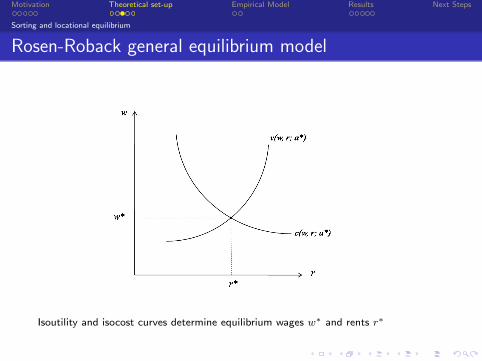
Rosen-Roback general equilibrium model
Isoutility and isocost curves determine equilibrium wages w∗ and rents r∗
Motivation Theoretical set-up Empirical Model Results Next Steps
Sorting and locational equilibrium
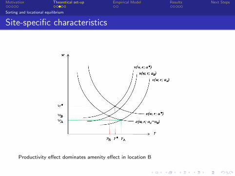
Site-specific characteristics
Location A has above-average amenities and below average productivity
Motivation Theoretical set-up Empirical Model Results Next Steps
Sorting and locational equilibrium
Site-specific characteristics
Productivity effect dominates amenity effect in location B
Motivation Theoretical set-up Empirical Model Results Next Steps
Sorting and locational equilibrium
Site-specific characteristics
Net effect on rents depends on relative shift of isoutility and isocost curves
Motivation Theoretical set-up Empirical Model Results Next Steps
Sorting and locational equilibrium
Classification by dominant effect
Relative importance of wage and rent compensating differentials
Motivation Theoretical set-up Empirical Model Results Next Steps
Sorting and locational equilibrium
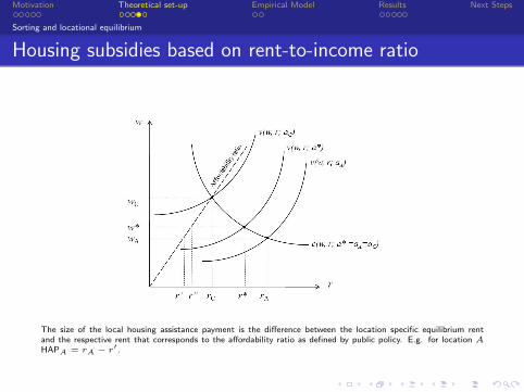
Housing subsidies based on rent-to-income ratio
The size of the local housing assistance payment is the difference between the location specific equilibrium rentand the respective rent that corresponds to the affordability ratio as defined by public policy. E.g. for location AHAPA = rA − r′.
Motivation Theoretical set-up Empirical Model Results Next Steps
Sorting and locational equilibrium
Urban rent and compensating differentials
Motivation Theoretical set-up Empirical Model Results Next Steps
Econometric approach
Two-stage estimator
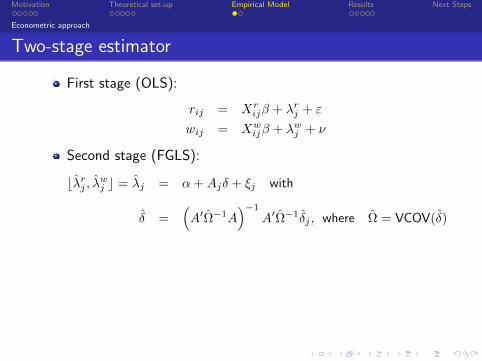
First stage (OLS):
rij = Xrijβ + λrj + ε
wij = Xwijβ + λwj + ν
Second stage (FGLS):
bλrj , λwj c = λj = α+Ajδ + ξj with
δ =(A′Ω−1A
)−1A′Ω−1δj , where Ω = VCOV(δ)
An atypical omitted variable problem with the goal to recoverthe composite index QOLIj , not marginal prices of individual
amenities δ
QOLIj =
K∑k=1
ajk
(δrk − δwk
)
Motivation Theoretical set-up Empirical Model Results Next Steps
Econometric approach
Two-stage estimator
First stage (OLS):
rij = Xrijβ + λrj + ε
wij = Xwijβ + λwj + ν
Second stage (FGLS):
bλrj , λwj c = λj = α+Ajδ + ξj with
δ =(A′Ω−1A
)−1A′Ω−1δj , where Ω = VCOV(δ)
An atypical omitted variable problem with the goal to recoverthe composite index QOLIj , not marginal prices of individual
amenities δ
QOLIj =
K∑k=1
ajk
(δrk − δwk
)
Motivation Theoretical set-up Empirical Model Results Next Steps
Data set
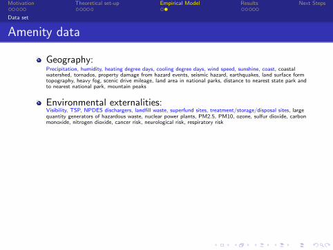
Amenity data
Geography:Precipitation, humidity, heating degree days, cooling degree days, wind speed, sunshine, coast, coastalwatershed, tornados, property damage from hazard events, seismic hazard, earthquakes, land surface formtopography, heavy fog, scenic drive mileage, land area in national parks, distance to nearest state park andto nearest national park, mountain peaks
Local public goods:Violent crime, teacher-pupil ratio, # schools, # public buildings, direct general expenditures, # hospitals,expenditures for hospitals and health, expenditures on parks and recreation, expenditures per student,private to public school enrollment, child mortality, museums and historical sites, zoos, botanical gardensand nature parks, campgrounds and camps
Cultural/urban amenities:Restaurants & bars, theatres & musicals, movie theatres, bowling alleys, amusement parks, research Iuniversities, golf courses and country clubs, military areas, distance to nearest urban center, distance tometro area, distance to metro area > 250k, distance to metro area > 500k, distance to metro area >1.5m, housing stress indicator, persistent poverty indicator, retirement destination indicator
Motivation Theoretical set-up Empirical Model Results Next Steps
Data set
Amenity data
Geography:Precipitation, humidity, heating degree days, cooling degree days, wind speed, sunshine, coast, coastalwatershed, tornados, property damage from hazard events, seismic hazard, earthquakes, land surface formtopography, heavy fog, scenic drive mileage, land area in national parks, distance to nearest state park andto nearest national park, mountain peaks
Local public goods:Violent crime, teacher-pupil ratio, # schools, # public buildings, direct general expenditures, # hospitals,expenditures for hospitals and health, expenditures on parks and recreation, expenditures per student,private to public school enrollment, child mortality, museums and historical sites, zoos, botanical gardensand nature parks, campgrounds and camps
Cultural/urban amenities:Restaurants & bars, theatres & musicals, movie theatres, bowling alleys, amusement parks, research Iuniversities, golf courses and country clubs, military areas, distance to nearest urban center, distance tometro area, distance to metro area > 250k, distance to metro area > 500k, distance to metro area >1.5m, housing stress indicator, persistent poverty indicator, retirement destination indicator
Motivation Theoretical set-up Empirical Model Results Next Steps
Distribution of HUD low-income housing subsidies
Notes: HUD subsidies are defined as the annual housing assistance payments (HAP) that bridge the gap betweenthe gross rent on a unit (FMR plus a 35% utility allowance) and the maximum total tenant payments (TTP) fora given household (capped at 30% of area median income for very-low income households). Average subsidies arecalculated using the FMRs for 1-bedroom (2-person family), 2-bedroom (4-person family), 3-bedroom (6-personfamily) and 4-bedroom (8-person family) units in combination with respective household-size specific income limitsthat are indicated in parentheses.
Motivation Theoretical set-up Empirical Model Results Next Steps
2-bedroom, 4-person family subsidy
Motivation Theoretical set-up Empirical Model Results Next Steps
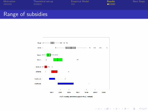
Range of subsidies
Motivation Theoretical set-up Empirical Model Results Next Steps
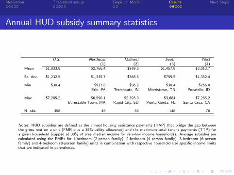
Annual HUD subsidy summary statistics
U.S. Northeast Midwest South West(1) (2) (3) (4)
Mean $1,833.8 $2,766.4 $979.8 $1,457.9 $3,013.7
St. dev. $1,232.5 $1,335.7 $368.8 $755.5 $1,352.4
Min $30.4 $937.8 $56.8 $30.4 $766.0Erie, PA Terrehaute, IN Morristown, TN Pocatello, ID
Max $7,285.2 $6,590.1 $2,393.9 $3,684 $7,285.2Barnstable Town, MA Rapid City, SD Punta Gorda, FL Santa Cruz, CA
N. obs. 358 45 89 148 76
Notes: HUD subsidies are defined as the annual housing assistance payments (HAP) that bridge the gap betweenthe gross rent on a unit (FMR plus a 35% utility allowance) and the maximum total tenant payments (TTP) fora given household (capped at 30% of area median income for very-low income households). Average subsidies arecalculated using the FMRs for 1-bedroom (2-person family), 2-bedroom (4-person family), 3-bedroom (6-personfamily) and 4-bedroom (8-person family) units in combination with respective household-size specific income limitsthat are indicated in parentheses.
Motivation Theoretical set-up Empirical Model Results Next Steps
HUD low-income housing subsidies and quality of life
Motivation Theoretical set-up Empirical Model Results Next Steps
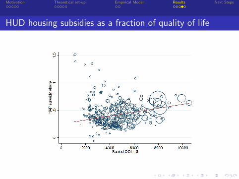
HUD housing subsidies as a fraction of quality of life
Motivation Theoretical set-up Empirical Model Results Next Steps
HUD housing subsidies as a fraction of quality of life
Motivation Theoretical set-up Empirical Model Results Next Steps
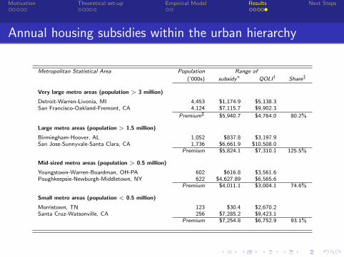
Annual housing subsidies within the urban hierarchy
Metropolitan Statistical Area Population Range of
(’000s) subsidy∗ QOLI† Share‡
Very large metro areas (population > 3 million)
Detroit-Warren-Livonia, MI 4,453 $1,174.9 $5,138.3San Francisco-Oakland-Fremont, CA 4,124 $7,115.7 $9,902.3
Premium] $5,940.7 $4,764.0 80.2%
Large metro areas (population > 1.5 million)
Birmingham-Hoover, AL 1,052 $837.8 $3,197.9San Jose-Sunnyvale-Santa Clara, CA 1,736 $6,661.9 $10,508.0
Premium $5,824.1 $7,310.1 125.5%
Mid-sized metro areas (population > 0.5 million)
Youngstown-Warren-Boardman, OH-PA 602 $616.8 $3,561.6Poughkeepsie-Newburgh-Middletown, NY 622 $4,627.89 $6,565.6
Premium $4,011.1 $3,004.1 74.6%
Small metro areas (population < 0.5 million)
Morristown, TN 123 $30.4 $2,670.2Santa Cruz-Watsonville, CA 256 $7,285.2 $9,423.1
Premium $7,254.8 $6,752.9 93.1%
Motivation Theoretical set-up Empirical Model Results Next Steps
Summary
Local variation in wages and prices imply significantinter-metropolitan differences in the ratio of income tohousing cost locational equilibrium.
Operationalizing housing affordability in terms of a nationalpolicy raises concerns from an allocational perspective.
Using unadjusted FMRs as a basis for allocating housingassistance is most problematic for larger metropolitan areaswhere amenity-driven compensating differentials play aparticularly important role.
Recognition that price-to-income ratios are affected by thelocation-specific attributes of housing markets providestransparent measure of housing affordability, directlyapplicable to a flexible menu of policy options.
Motivation Theoretical set-up Empirical Model Results Next Steps
Future work
Amenity expenditures do not measure social welfare. Bounds?