Housing and Macroeconomics∗

Monika Piazzesi

Stanford & NBER

Martin Schneider

Stanford & NBER

July 2016

Abstract

This paper surveys the literature on housing in macroeconomics. We first collect facts

on house prices and quantities in both the time series and the cross section of households

and housing markets. We then present a theoretical model of frictional housing markets

with heterogeneous agents that nests or provides background for many studies. Finally,

we describe quantitative results obtained during the last 15 years on household behavior,

business cycle dynamics and asset pricing, as well as boom bust episodes.

JEL Codes: R2, R3, E2, E3, E4, G1

∗Email addresses: piazzesi@stanford.edu, schneidr@stanford.edu. We thank Alina Arefeva, Eran Hoffmann,Amir Kermani, Moritz Lenel, Sean Myers, Alessandra Peter, John Taylor, Harald Uhlig, and conference partic-

ipants at Stanford for comments.

1

1 Introduction

The first volume of the Handbook of Macroeconomics, published in 1999, contains essentially

no references to housing. This statistic accurately summarizes the state of the field at the

time. Of course, housing was not entirely absent from macroeconomic studies, which typically

account for all production, consumption and wealth in an economy. The lack of references

instead reflected the treatment of housing as simply one component of capital, consumption or

household wealth that does not deserve special attention.

At the turn of the millennium, housing was implicitly present in three loosely connected

literatures. One is work on aggregate fluctuations that studies the sources of business cycles

and the response of the economy to fiscal and monetary policy. In the typical 20th century

model, residential structures were part of capital, or sometimes “home capital” (together with

consumer durables). Housing services were part of nondurables (or home good) consumption.

Models of financial frictions and the role of capital as collateral focused on borrowing by firms.

Volatility of house prices played no role — in fact, any volatility of asset prices was largely a

sideshow.

Second, housing was implicitly present in the large body of work on asset pricing concerned

with differences in average returns and price volatility across assets. Studies in this area used

to largely stay away from properties of house prices and returns. At the same time, a common

modeling exercise identified a claim to all consumption with equity and tried to explain the

volatility of its price with a consumption-based stochastic discount factor. Housing thus played

an implicit role as part of payoffs and risk adjustment. Finally, there is work on heterogenous

households that seeks to understand the role of frictions and policy for inequality as well as

distributional effects of shocks. Here housing was included as a large implicit component of

household wealth as well as a share of consumption.

The first half of the 2000s saw not only the largest housing boom in postwar U.S. history,

but also new research that introduced an explicit role for housing in macroeconomics. The new

research studies the interaction of house prices and collateralized household borrowing with

business cycles and monetary policy. It also explores how the role of housing as a consumption

good as well as a collateralizable asset affects savings, portfolio choice and asset pricing. By

the time the U.S. housing boom turned into a spectacular bust in 2007, housing was already

a prominent topic in macroeconomics. The Great Recession added important new data points

and further underscored the importance and unique properties of housing. As a result, housing

now routinely receives special attention in macroeconomic discussions.

While the new literature grew out of the three lines of research described above, the focus on

housing brought out several distinctive features. First, it naturally pushed researchers towards

integration of themes and tools from all three lines of research. It is difficult to describe house-

hold behavior while ignoring uncertainty about house prices, or to think about mortgage debt

without heterogeneous agents. Many papers surveyed below thus employ tools from financial

economics to study exposure to uncertainty, and many quantitative models are analyzed with

computational techniques that allow rich heterogeneity within the household sector.

The second feature is familiar from urban economics: “the housing market” is really a col-

lection of many markets that differ by geography as well as other attributes. Disaggregating

2

not only the household sector but also the housing stock provides valuable insights into the

transmission of shocks and alters policy conclusions. For example, shocks to financial interme-

diaries or policies that change the cost of mortgage credit might have stronger effects on prices

in markets where the typical buyer is also a borrower. Moreover, those shocks might have larger

aggregate effects if their impact cannot be shared across subpopulation of agents. Availability

of new large scale micro data sets has made it possible to explicitly study the interactions of

many agents in many markets, and derive the aggregate effects of those interactions.

A third, related, feature is that the literature on housing has brought to bear a lot of evidence

from the cross section of markets in a single episode to complement time series evidence that

is common in macroeconomics. To illustrate, one can learn a lot about the role of technology

shocks for residential investment from recurrent time series patterns in postwar history. In

contrast, to assess the role of recent financial innovation for house prices, such patterns are less

informative. Fortunately, though, we can learn from cross sectional patterns in financing and

prices across submarkets and types of households.

The literature shows how both time series and cross sectional patterns on housing markets

lend themselves to the same style of analysis that is common elsewhere in macroeconomics.

Reduced form statistical tools are used to document facts and sometimes to isolate certain

properties of equilibrium relationships. Insights on the quantitative importance of different

mechanisms as well as policy counterfactuals are derived from multivariate structural models.

In many ways, modeling the cross-sectional comovement in a single period of, say, mortgage bor-

rowing and wealth across households and house prices across market segments, is conceptually

similar to modeling the time series comovement of, say, residential and business investment,

GDP and house prices in postwar history. Both exercises require tracing out the effect of

exogenous variation in some features of the environment jointly on many endogenous variables.

This chapter describes work on housing in macroeconomics in three parts. Part I collects the

new facts that emerge once disaggregation makes housing explicit. We first document business

cycle properties of housing consumption, residential investment and mortgage debt. We then

look at the dynamics of house prices at the national, regional and within-city level, and compare

price volatility and trading volume for housing and securities. Finally, we document the dual

role of housing as a consumption good as well as an asset in household portfolios.

Part II describes a theoretical framework that nests or provides background for many studies

in the literature. It allows for four special features of housing that are motivated by facts from

Part I: indivisibility, nontradability of dividends, illiquidity and collateralizability. Indeed, many

homeowners own only their residence, directly consume its dividend in form of housing services

and bear its idiosyncratic risk. Moreover houses are relatively costly to trade and easy to pledge

as collateral. In contrast, securities such as equity and bonds are typically held in diversified

portfolios, have tradable payoffs, are traded often at low cost, and are harder to use as collateral.

Part III summarizes quantitative results derived from versions of the general framework over

the last two decades or so. While no study contains all the ingredients introduced in Part II,

each one quantifies one or more of the tradeoffs discussed there. We start by reviewing work on

consumption, savings and portfolio choice. We also consider mortgage choice and the role of

financial innovation for household decisions. We then move on to general equilibrium analysis of

the business cycle, monetary policy and asset prices. Finally, we consider boom-bust episodes,

3

with an emphasis on the 1970s and 2000s U.S. housing cycles.

We interpret results from different types of quantitative exercises in light of the general

framework. One approach studies structural relationships with an explicit shock structure. For

example, large bodies of work assess the ability of lifecycle models of consumption, savings and

portfolio choice to explain cross sectional patterns as well as the ability of DSGE models to

match time series patterns. An alternative approach investigates families of Euler equations

for different agents and/or markets to reconcile allocations and asset prices. A third approach

tries to isolate properties of the decision rules or the equilibrium law of motion with reduced

form approaches.

What have we learned so far? We highlight here two key takeaways from the new litera-

ture that underlie the quantitative successes reported in detail below. First, frictions matter.

Quantitative modeling of household behavior now routinely relies on collateral constraints, in-

complete markets and transaction costs as key ingredients. Incompleteness of markets means

in particular that homeowners bear property-level price risk. A large body of reduced form

evidence provides additional support for this approach. Second, heterogeneity of households

matters. Models with heterogeneous households and frictions introduce powerful new amplifi-

cation and propagation mechanisms. In particular, they provide more scope for effects of shocks

to the financial sector which have become important in accounts of postwar U.S. history, espe-

cially the recent boom-bust cycle.

We also conclude that making housing explicit improves our understanding of classic macro-

economic questions, previously studied only with models that provide an implicit role for hous-

ing. For thinking about business cycles, the comovement and relative volatility of residential

and business investment provide discipline on model structure. For thinking about asset pric-

ing, the role of housing as a consumption good as well as a collateralizable asset generate the

type of slow moving state variables for model dynamics that are needed in order to understand

observed low frequency changes in the risk return tradeoffs for many assets, including hous-

ing itself. Finally, financial frictions in the household sector change the transmission of both

aggregate and distributional shocks and policy interventions, especially to consumption.

At the same time, many open questions remain and there is ample opportunity for future

research. One issue is the tradeoff between tractability and detail faced by any macroeconomic

study. There are three areas in particular where more work is needed to converge on the

right level of abstraction — with possibly different outcomes depending on the question. One is

aggregation across housing markets: do we gain, for example, from building more models that

treat the U.S. as a collection of small countries identified with, say, states or metropolitan areas?

Another area is choosing dimensions of household heterogeneity: since observable demographic

characteristics such as age, income and wealth explain only a small share of cross sectional

variation, how should unobservable heterogeneity be accommodated? Finally, the majority of

studies reviewed below capture financial frictions by assuming short term debt and financial

shocks as changes to maximum loan-to-value ratios. Given the rich and evolving contractual

detail we see in the data, what are the essential elements that should enter macroeconomic

models?

A major outstanding puzzle is the volatility of house prices — including but not only over

the recent boom-bust episode. Rational expectations models to date cannot account for house

4

price volatility — they inevitably run into “volatility puzzles” for housing much like for other

assets. Postulating latent "housing preference shocks" helps understand how models work when

prices move a lot, but is ultimately not a satisfactory foundation for policy analysis. Moreover,

from model calculations as well as survey evidence, we now know that details of expectation

formation by households — and possibly lenders and developers — play a key role. A promising

agenda for research is to develop models of expectation formation that can be matched to data

on both market outcomes and survey expectations. A final point is that most progress we

report is in making sense of household behavior. The supply side of housing as well as credit

to fund housing has received relatively less attention, another interesting direction for future

work.

To keep the length of chapter manageable, we have narrowed focus along some dimensions

where other recent survey papers already exist. In particular, the Handbook of Urban and

Regional Economics contains chapters on search models of housing (Han and Strange, 2015) as

well as U.S. housing policy (Olsen and Zabel, 2015).1 Since we focus on work that is already

published, we have also left out much of the important emerging literature on the housing

bust and Great Recession, as well as policy at the zero lower bound for nominal interest rates.

Finally, our chapter deals almost exclusively with facts and quantitative studies about the

United States. This reflects the focus of the literature, which in turn has been driven in part

by availability of data. Another exciting task for future research is to use the tools discussed

in this chapter to study the large variation in housing market structure and housing finance

across countries, surveyed for example by Badarinza, Campbell and Ramadorai (2016).

Part I

Part I: facts

2 Quantities

Figure 1 plots the aggregate expenditure share on housing from the National Income and

Product Account (NIPA) tables. The numbers in NIPA table 2.3.5 are based on survey data.

The questionnaires in these surveys (for example, the Residential Finance Survey conducted by

the Census Bureau) ask renters about their actual monthly rent payments. These payments are

imputed to comparable owner-occupied units (Mayerhauser and Reinsdorf 2007.). The sample

consists of quarterly data from 1959:Q1 to 2013:Q4.

We compute the expenditure share in two ways. The blue line shows housing expenditures

as a fraction of expenditures on nondurables and services. This series has a mean of 21 percent

and a standard deviation of 0.061 percent. The green line shows housing services as a fraction

of total consumption (including durables). This series has a slightly lower mean of 17.8 percent

and a bit higher standard deviation of 0.064 percent. The yellow bars indicate NBER recessions.

1The same handbook contains a chapter on housing, finance and the macroeconomy (Davis and Van Nieuwer-

burgh, 2015) that also discusses some of the material covered in the present chapter.

5

1960 1970 1980 1990 2000 20100

0.05

0.1

0.15

0.2

0.25

0.3

0.35

0.4nondur & services, mean 21.0%, std dev 0.061%total consumption, mean 17.8%, std dev 0.064%

Figure 1: Aggregate expenditure share on housing, 1959:Q1-2014:Q4.

The overall impression from Figure 1 is that the aggregate expenditure share is pretty

flat over time. The expenditure share on housing is also similar across households in micro

data, as shown by Piazzesi, Schneider and Tuzel (2007). Their Table A.1 shows evidence from

the Consumer Expenditure Survey, where the definition of housing expenditures depends on

tenure choice. The CEX asks renters about their rent payments, while owner occupiers are

asked about their interest payments on mortgages and other lines of credit, property taxes,

insurance, ground rents, and expenses for maintenance or repairs. Davis and Ortalo-Magne

(2011) use micro data on the expenditure share of renter households alone. The paper shows

that individual expenditure shares based on the 1980, 1990 and 2000 Decennial Housing Surveys

do not vary much within or across the top 50 U.S. metropolitan statistical areas.

Figure 2 plots three series: residential investment, nonresidential investment and output.

The series are from NIPA table 1.1.3; they are all logged and detrended using the Hodrick-

Prescott filter. The figure illustrates that both investment series are more volatile than output.

Also, residential investment is twice as volatile as nonresidential investment. The volatility of

residential investment is 9.7 percent, while nonresidential investment has a volatility of 4.6

percent and the volatility of output is 1.6 percent. The figure also shows that the series for

residential investment tends to increase before nonresidential investment and output, and it

tends to decrease before the other two series. In other words, residential investment leads the

cycle.

Once investment has created housing capital, it stays around for a long time. As reported by

Fraumeni (1997), structures depreciate at rates of 1.5 to 3 percent per year. The depreciation

6

1960 1970 1980 1990 2000 2010

-0.3

-0.2

-0.1

0

0.1

0.2

0.3

residential inv σ=9.7%nonresidential inv σ=4.6%output σ=1.6%

Figure 2: Aggregate residential investment, nonresidential investment and output; logged and

detrended with Hodrick-Prescott filter.

rates for nonresidential capital are higher, between 10 and 30 percent. Moreover, housing

combines housing capital with land, which is a fixed factor.

Constraints on the supply of housing

The degree to which new developments can increase the supply of housing varies across

geographic areas. For example, developers in Indianapolis and Omaha find it easier to buy

land and construct new homes than developers in San Francisco and Boston. There are two

popular indices that carefully measure such housing supply constraints.

The first index is by Saiz (2010) and captures physical constraints. These geographical

constraints capture two main features of land topology that make new developments difficult

or impossible. The first feature is the presence of water. Saiz measures the area within 50

kilometers from cities that is covered by oceans, lakes, rivers, and other water bodies such as

wetlands. The second feature of land topology is steep slopes. Saiz computes the share of the

area with a slope above 15 percent within a 50 kilometer radius around an MSA.

The second measure of supply constraints captures regulatory restrictions. These are mea-

sured by the Wharton Residential Urban Land Regulation Index created by Gyourko, Saiz, and

Summers (2008). This index captures the stringency of residential growth controls in terms of

zoning restrictions or project approval practices.

7

1960 1970 1980 1990 2000 201020

30

40

50

60

70

5

10

15

20stock price/dividendshouse price/rents

Figure 3: Aggregate price/dividend ratio for stocks and price/rent ratio for housing

3 Prices

Figure 3 shows the price-dividend ratio for stocks as a green line which measured on the left axis.

The figure also shows the price-rent ratio for housing as a blue line with units indicated on the

right axis. The figure illustrates the large volatility of the two series. The price-dividend ratio

for stocks uses data from the Flow of Funds and represents the overall valuation of companies

in the United States. The dividend series includes net repurchases. The price-dividend ratio

fluctuates between 20 and 65, as measured on the left axis.

The numerator of the price-rent series for housing is the value of residential housing owned

by partnerships, sole proprietors, and nonfinancial corporations, which are landlords for many

rental units, as measured by the Flow of Funds. The denominator of the price-rent series is

rents from the NIPA table 2.3.5, which includes actual rent payments as well as imputed rents

for owner-occupiers (as discussed in the context of Figure 1). The price-rent ratio fluctuates

between 11 and 19, as measured on the right axis.

The two valuation ratios often move inversely. For example, stocks tanked during the

housing booms in the 1970s and 2000s. By contrast, stocks appreciated during the 1990s

while housing did poorly. The recent boom-bust episode in housing stands out in the postwar

experience.

Excess volatility of individual house prices

House prices, like the prices of other assets, are highly volatile. The prices of individual

8

houses are especially volatile. The volatility of various house price indices is smaller, but still

a challenge for economic models — this is the excess volatility puzzle.

Most house price indices are constructed from repeat sales — average price changes in houses

that sell more than once in the sample. CoreLogic constructs such city-wide indices for many

metropolitan areas, various tiers of these markets, as well as the U.S. national index. These

indices are published as the S&P/Case-Shiller Home Price Indices by Standard & Poor’s. The

Federal Housing Finance Agency also constructs such indices from repeat sales or refinancings

on the same properties (formerly called the OFHEO index). Zillow also publishes such indices

for cities, states or the nation.

Case and Shiller (1989) estimate the standard deviation of annual percentage changes in

individual house prices to be close to 15%. The paper concludes that individual house prices

are similar to individual stock prices that are also very volatile. City-wide indices are less

volatile than individual house prices. Flavin and Yamashita (2002) estimate a 14% volatility

for individual house prices in their Table 1A. Their Table 1B reports a 4% volatility for Atlanta,

6% for Chicago, 5% for Dallas and 7% for San Francisco. Landvoigt, Piazzesi and Schneider

(2015) estimate the volatility of individual house prices in different years. Their Table 1 shows

estimates that range between 8-11% during the 2000s boom and 14% during the bust.

Compared to stocks, which commove strongly with the aggregate stock market, a larger

share of the volatility in individual house prices is idiosyncratic, as documented in Case and

Shiller (1989). Their evidence stems from regressions of individual house price change on city-

wide price changes. The regressions have low 2s: 7% for Atlanta, 16% for Chicago, 12% for

Dallas, and 27% for San Francisco.

Table 1 summarizes information from Tables B1 and B2 from Piazzesi, Schneider and Tuzel

(2007). The table illustrates the rule of thumb that 1/2 of the volatility in individual house

prices is city-level variation, while 1/4 of the individual volatility is aggregate house price

variation. This volatility decomposition illustrates the importance to understand the variation

within narrow locations or individual houses. The high volatility of individual house prices

together with high transaction costs lead to low Sharpe ratios (defined as average excess return

on an asset, divided by its volatility) on housing. In other words, individual houses are not as

attractive as an investment.

Table 1: House price volatility

individual house city state aggregate

volatility 14% 7% 5% 2-3%

Note: This table is from Tables B1 and B2 in Piazzesi, Schneider and Tuzel (2007).

Idiosyncratic shocks to house prices are difficult to diversify. The problem with houses is

that they are indivisible — they are sold in their entirety, not in small pieces. As a consequence,

households own 100% of a specific house rather than small portions of many different houses.

Moreover, the market for housing indices is not very liquid. In any given month, only a couple

9

of futures contracts on city-wide house price indices trade on the Chicago Mercentile Exchange,

if they trade at all.2

The ease of diversification distinguishes houses from other assets such as stocks. For exam-

ple, households can save a small amount of money and invest it in a stock market index (such

as the S&P 500) that tracks the value of a large stock portfolio. Alternatively, households can

buy a few shares from several companies. The conventional wisdom in finance is that a small

number of different stocks — such as five or six companies — are sufficient to achieve a high

degree of diversification in a portfolio.

Momentum and reversal

House prices have more momentum than other assets and also exhibit long-run reversal.

The changes in log real prices of houses are more highly serially correlated compared to other

assets. Case and Shiller (1989) provide the first evidence of such high serial correlation. They

document that a change in the log real price index in a given year and a given city tends to be

followed by a change in the same direction the following year between 25% and 50% as large.

Englund and Iaonnides (1997) provide cross-country evidence where changes are followed by

changes between 23% and 74% the next year. Glaeser, Gyourko, Morales and Nathanson (2014)

find changes the next year between 60% and 80%.

Cutler, Poterba and Summers (1991) compare the serial correlation in housing markets to

that in other asset markets across many countries. For example, stocks, bonds and foreign

exchange exhibit weak momentum for horizons less than a year. The monthly autocorrelation

in excess stock returns is 10%, for U.S bonds it is 3%, 24% for foreign bonds, and 7% for foreign

exchange. The excess returns on all these assets are essentially uncorrelated from year to year.

In contrast, the excess returns on housing in their Table 4 has an autocorrelation of 21% from

year to year.

Over longer periods, house prices experience reversal. Englund and Ioannides (1997) doc-

ument that changes in log real prices are followed by changes in the opposite direction after

five years. Glaeser et al. (2014) also provide evidence of such reversal in their Table 4. They

estimate the autocorrelation of real house price changes over five years to be −080Predictable excess returns on housing

The excess returns on many assets, including housing, are predictable. Case and Shiller

(1989) show that excess returns on the city indices are predictable with excess returns in the

previous year in their Table 3. Case and Shiller (1990) provide further evidence of predictability

for excess returns. Their Table 8 runs regressions of city excess returns on rent-price ratios and

construction costs divided by price. The coefficient on the rent-price ratio is positive: a high

rent-price ratio predicts high excess returns over the next year.

Cochrane (2011) compares the predictability regressions for houses and stocks. Table 2 here

replicates his Table 3. “Houses” in Table 2 refers to the aggregate stock of housing in the

United States. “Stocks” refers to a value-weighted index of U.S. stocks. The estimated slope

coefficients indicate that high rents relative to prices signal high subsequent returns, not lower

2The data on volume in these markets is here http://www.cmegroup.com/market-data/volume-open-

interest/real-estate-volume.html

10

subsequent rents. The results for housing in the left panel look remarkably similar to those in

the right panel for stocks. The returns are predictable for both, but dividend growth and rent

growth are not predictable. The ratio of rents or dividends to prices is highly persistent, but

stationary.

Table 2: House Price and Stock Price Regressions

Houses Stocks

2 2

+1 0.12 (2.52) 0.15 0.13 (2.61) 0.10

∆+1 0.03 (2.22) 0.07 0.04 (0.92) 0.02

+1 0.90 (16.2) 0.90 0.94 (23.8) 0.91

Note: This table is Table 3 from Cochrane (2011). It reports results from regressions

of the form

+1 = + × + +1

where is either the log rent-price ratio in the left panel or the log dividend-

price ratio in the right panel. In the left panel, +1 is either log annual housing

returns +1, log rent growth ∆+1, or the log rent-price ratio +1 measured

with annual data for the aggregate stock of housing in the United States, 1960-

2010, from http://www.lincolninst.edu/subcenters/land-values/rent-price-ratio.asp

In the right panel, +1 is either log stock returns +1, dividend growth ∆+1 ,

or the log dividend-price ratio +1 measured with annual CRSP value-weighted

return data, 1947-2010.

Campbell, Davis, Gallin, and Martin (2009) decompose house price movements with the

Campbell-Shiller linearization of the one-period return

+1 ≈ const. + (+1 − +1)− ( − ) +∆+1

where +1 = log+1 is the log housing return, = log () is the log house price, = log ()

is the log rent, ∆+1 = +1− is rent growth and = 098 is a constant in the approximation.This return identity simply says that high returns either come from higher prices (future −),lower initial prices, or higher dividends.

By iterating the return identity forward, we get the present value identity

≈ const. +X

=1

−1+ −X

=1

−1∆+ + + (1)

where = − is the log rent-price ratio. The present value identity holds state-by-state

as well as in expectation. Any movement in the rent-price ratio on houses therefore has to

be associated with a movement in either the conditional expected value of future returns +,

expected future rent growth ∆+ or a bubbly anticipation of future high prices +.

11

Campbell et al. estimate a vector-autoregression that includes real interest rates, rent

growth and excess returns on housing. The housing data are from various metropolitan regions

and U.S. aggregate data. Based on the estimated VAR, the paper evaluates the expected

infinite sums of future returns and future rent growth on the right-hand side of equation (1) for

→∞ by imposing the no-bubble condition3 lim→∞ + = 0. It finds that movements in

price-rent ratios can be attributed to a large degree to time variation in risk premia and less so

to expectations of future rent growth. The time variation in real interest rates does not explain

price-rent ratio movements. Their Figure 2 also shows that the 2000s boom is hard to explain

through the lense of their estimated VAR which predicts low price-rent ratios throughout the

2000s.

Value of land versus structures

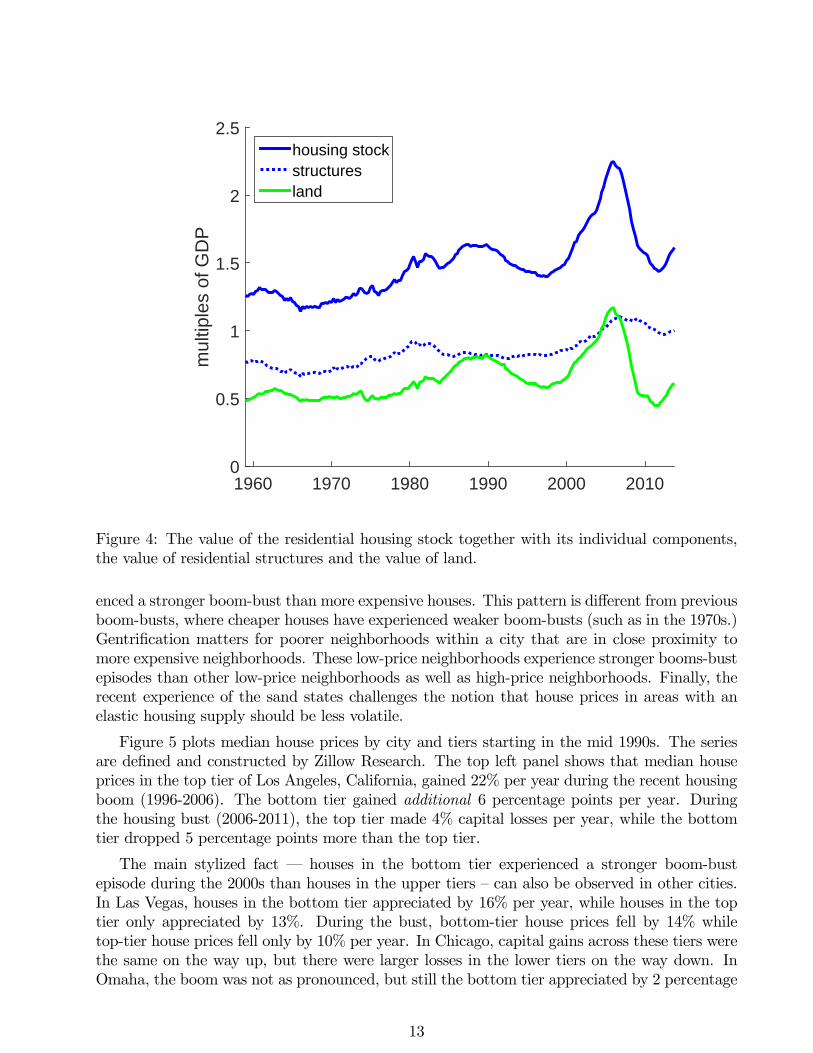
Figure 4 plots the value of the residential housing stock together with its two components,

the value of the residential structures and the value of land. All series are from the Flow of

Funds and are reported as multiples of GDP. The figure illustrates that movements in the value

of the residential housing stock are mostly due to movements in the value of land. The value

of structures fluctuates much less. The figure again highlights the importance of the recent

boom-bust episode in the postwar housing experience.

Knoll, Schularick and Steger (2014) collect data on house values in many industrialized

countries going back to 1870. The paper documents that real house values in most countries

were largely constant from the 19th to the mid 20th century. Over the postwar period, real house

prices approximately tripled. The majority of this increase in real house prices is associated

with rising land prices, while real construction costs have been roughly constant.

There is also large cross sectional variation in the share of land in the overall house value. A

key component of this variation is what realtors call “location, location, location”: each location

is unique. There may be attractive locations with unique characteristics in fixed supply such

as lake- and oceanfronts, locations with strict zoning rules, outstanding amenities such as good

schools or opera houses, low crime etc. For example, Table 4 in Davis and Heathcote (2007)

reports that houses in San Francisco have a land share of 80.4% while houses in Oklahoma City

have a land share of 12.6%. The table shows that areas with higher land shares tend to have

higher house prices, higher average house price growth and more volatile house prices.

Another source of cross sectional variation are differences in the durability and/or attractive-

ness of the existing structures. For example, the building material for structures in earthquake

prone areas like California tends to be wood, which is cheaper and deteriorates faster than brick

which is used for most constructions in Pennsylvania. Architectural styles may also matter.

For example, Victorian homes are valued at a premium, while 1950s postwar structures come

at a discount.

Cross section of house prices

There are important cross sectional patterns in house prices that help understand the vari-

ation across and within narrow areas. For example, during the 2000s, cheaper houses experi-

3Giglio, Maggiori and Stroebel (2016) provide direct evidence on the no-bubble condition in housing markets

by comparing the value of freeholds (infinite maturity ownerships of houses) with the value of leaseholds with

maturities over 700 years in the U.K. and Singapore.

12

1960 1970 1980 1990 2000 2010

mul

tiple

s of

GD

P

0

0.5

1

1.5

2

2.5housing stockstructuresland

Figure 4: The value of the residential housing stock together with its individual components,

the value of residential structures and the value of land.

enced a stronger boom-bust than more expensive houses. This pattern is different from previous

boom-busts, where cheaper houses have experienced weaker boom-busts (such as in the 1970s.)

Gentrification matters for poorer neighborhoods within a city that are in close proximity to

more expensive neighborhoods. These low-price neighborhoods experience stronger booms-bust

episodes than other low-price neighborhoods as well as high-price neighborhoods. Finally, the

recent experience of the sand states challenges the notion that house prices in areas with an

elastic housing supply should be less volatile.

Figure 5 plots median house prices by city and tiers starting in the mid 1990s. The series

are defined and constructed by Zillow Research. The top left panel shows that median house

prices in the top tier of Los Angeles, California, gained 22% per year during the recent housing

boom (1996-2006). The bottom tier gained additional 6 percentage points per year. During

the housing bust (2006-2011), the top tier made 4% capital losses per year, while the bottom

tier dropped 5 percentage points more than the top tier.

The main stylized fact – houses in the bottom tier experienced a stronger boom-bust

episode during the 2000s than houses in the upper tiers — can also be observed in other cities.

In Las Vegas, houses in the bottom tier appreciated by 16% per year, while houses in the top

tier only appreciated by 13%. During the bust, bottom-tier house prices fell by 14% while

top-tier house prices fell only by 10% per year. In Chicago, capital gains across these tiers were

the same on the way up, but there were larger losses in the lower tiers on the way down. In

Omaha, the boom was not as pronounced, but still the bottom tier appreciated by 2 percentage

13

2000 2005 2010 2015

Tho

usan

ds o

f Dol

lars

200

400

600

800

100022%

27%

28%

-4%

-7%

-9%

Los Angeles, CA

2000 2005 2010 2015

100

200

300

400

500 13%

14%

16%-10%

-12%

-14%

Las Vegas, NV

2000 2005 2010 2015

Tho

usan

ds o

f Dol

lars

100

200

300

40012%

12%

12%

-4%

-6%

-6%

Chicago, IL

2000 2005 2010 2015

100

200

300

400

500

3%

4%5%

0%

0%-1%

Omaha, NE

Figure 5: Median house prices (in thousands of Dollars) by city and tier: top tier (red line),

medium tier (magneta line) and low tier (blue line). The data are from Zillow Research. The

colored numbers indicate the tiered capital gains in percent per year during the housing boom

(1996-2006) and during the bust (2006-2011).

points more than the top tier and was the only tier to experience a capital loss during the bust.

Landvoigt, Piazzesi and Schneider (2015) estimate these patterns for the metro area of San

Diego based on individual transaction data. The paper documents a roughly 20% difference

between capital gains on the cheapest houses and most expensive houses between the years 2000

and 2005. The Zillow tiers group the cross section of houses and thereby reduce these cross-

sectional differences. Kuminoff and Pope (2013) show a similar pattern for the land component

of house values: cheap land appreciated more than expensive land during the 2000s boom.

Hartley, Hurst and Guerrieri (2013) document that gentrification matters for poorer neigh-

borhoods that are geographically close to high-price neighborhoods within a city. Their Table 3

shows that neighborhoods with an initially low price which were in close promixity to high-price

neighborhoods appreciated more than otherwise similar initially low-price neighborhoods. For

example, low-priced neighborhoods that were roughly 1 mile away from high-price neighbor-

hoods appreciated by 12.4 percentage points more than low-priced neighborhoods that were

roughly 4 miles away.

The recent experience in the “sand states”–Arizona, Florida, Nevada and inland California–

14

1960 1970 1980 1990 2000 2010

Mul

tiple

s of

GD

P

0

0.2

0.4

0.6

0.8

1mortgage debtall household debt

Figure 6: Aggregate household debt and mortgage debt as fraction of GDP

has challenged the notion that supply constraints amplify house price cycles. Figure 1 in David-

off (2013) shows that the magnitude of the house price cycle in the early 2000s in the sand states

was larger than the cycle in coastal markets. His Figure 2 documents that the increase in the

number of housing units was also larger in the sand states. Nathanson and Zwick (2015) argue

that some cities, such as Las Vegas, do not have an abundance of land. Instead, these cities

face long-run supply constraints in the form of tight virtual urban growth boundaries, formed

by encircling federal and state lands.

4 Financing

Figure 6 shows aggregate household debt from the Flow of Funds as multiple of GDP in the

United States over the postwar period. The increase in the series happened in three discrete

steps: right after World War II, the 1980s, and the 2000s. After the collapse of the housing

market in 2006, households have been deleveraging. The red line in Figure 6 is mortgage

debt/GDP, which is roughly 3/5 of overall household debt. Most of household debt is thus

collateralized. The plot shows that mortgage debt is chiefly responsible for the three discrete

steps in which debt drastically increased. Household debt, especially mortgage debt, has also

increased in other countries over the postwar period, as documented by Cardarelli, Igan and

Rebucci (2008). Jordà, Schularick and Taylor (2016a) document this increase for many indus-

trialized countries in a sample that goes back to 1870.

Jordà, Schularick and Taylor (2016b) document that asset price boom-bust episodes that are

combined with prior run-ups in leverage are associated with larger output costs during their

bust. The data sample covers many industrialized countries going back to 1870. Moreover,

boom-busts in housing have more severe output costs than those in equity markets.

15

Mortgage growth during the 2000s

Mian and Sufi (2009) investigate who borrowed more during the 2000s. Did these borrowers

expect higher future income growth? To address this question, Mian and Sufi use IRS data on

income and mortgage debt data from the “Home Mortgage Disclosure Act” (HMDA). Their

Figure 1 shows that income growth and mortgage growth are positively correlated across metro

areas between 2002 and 2005 (in their top right panel). The evidence within metro areas,

however, shows a negative correlation between income growth and mortgage growth across zip

codes (in the lower right panel.) Moreover, they show that this negative correlation at the zip

code level is unique to the 2002-2005 period. These findings suggest that the 2000s were a

unique episode in which mortgage debt increased in zip codes that experienced lower income

growth.

Adelino, Schoar and Severino (2015) decompose mortgage growth into the extensive margin

— the growth rate in the number of mortgages in a zip code — and the intensive margin — the

growth rate in the size of individual mortgages. Their Table 2 shows that the extensive margin

is responsible for the negative correlation between IRS income growth and mortgage growth

across zip codes. In fact, the intensive margin is positively correlated with IRS income at the

zip code level. Moreover, Adelino et al. show that the growth rate of individual HMDA income

– borrowers’ income as indicated on their mortgage applications – is positively correlated to

individual mortgage size across households. The paper argues that the negative correlation

between income and mortgage growth documented by Mian and Sufi (2009) may be explained

by a change in buyer composition (i.e. richer buyers in poorer zip codes).

Mian and Sufi (2015) present evidence that the growth rate of HMDA income is higher than

IRS reported income growth at the zip code level. They argue that the difference between the

two growth rates represents mortgage fraud. Of course, the comparison of HMDA income and

IRS income is tricky, because mover households who purchase a home have different character-

istics than stayer households, especially during the 2000s boom. Table 2 in Landvoigt, Piazzesi

and Schneider (2015) compares the characteristics of home buyers and homeowners in 2000

Census data and 2005 data from the American Community Survey. They find that the median

buyer in 2005 has more income and is richer than in 2000 in real terms.

Another important component of the increase in mortgage debt are existing homeowners

who borrowed against the increased value of their house. Mian and Sufi (2011) document that

especially homeowners in areas with stronger house price appreciation extracted equity from

their houses with home equity lines of credit. Chen, Michaux and Roussanov (2013) report

that a large fraction of refinancing during the 2000s were cash-outs, defined as more than 5%

increases in loan amounts.

Mortgage contracts

In the United States, the predominant mortgage contract is a fixed-rate mortgage with

long maturity, usually 30 years. The main alternative is an adjustable-rate mortgage. In a

basic adjustable-rate mortgage, the initial rate is set as a markup (or margin) on top of a

benchmark, such as the one-year Treasury rate. Adjustable rates are periodically reset to the

current benchmark. During the recent housing boom, hybrid adjustable-rate mortgages became

more popular. These hybrid contracts have a fixed rate for an initial period up to 10 years and

16

adjusted periodically thereafter.

Campbell and Cocco (2003) report that fixed-rate mortgages accounted for 70 percent of

newly issued mortgages on average during the period 1985-2001, while adjustable-rate mort-

gages accounted for the remaining 30 percent. The share of fixed-rate mortgages in new origi-

nations fluctuates over time. Figure 2 in Campbell and Cocco (2003) shows the evolution of the

share of fixed-rate mortgages, which is strongly negatively correlated with long-term interest

rates.

Cardarelli, Igan and Rebucci (2008), Andrews, Caldera Sánchez and Johansson (2011) and

Badarinza, Campbell and Ramadorai (2016) provide cross-country evidence on mortgage con-

tracts. Table 4 in Andrews et al. shows that the typical mortgage maturity varies across

countries between 10 years in Slovenia and Turkey to 30 years in Denmark and the United

States. Table 3 in Badarinza et al. shows wide differences in the use of adjustable-rate mort-

gages and prepayment penalties. For example, the majority of mortgages in Australia, Finland,

Portugal and Spain have an adjustable rate, while Belgium, Denmark, Germany and the U.S.

have mostly fixed-rate mortgages. Belgium and Germany have prepayment penalties, which

make these fixed-rate mortgages highly risky. Table 3.1 in Cardarelli et al. (2008) shows that

the countries with the largest fractions of securitized mortgages are the U.S., Australia, Ireland,

Greece, U.K. and Spain.

Recent financial innovation and lender incentives

Leading up to the recent housing boom, the banking sector underwent a profound trans-

formation. The traditional role of banks was to originate mortgages and hold them on their

books until they are repaid. More and more, modern banks “originate-to-distribute”; banks

originate mortgages, pool and tranch them, and resell them in the securitization process. In

other words, mortgages are not kept on the balance sheet of the originating bank but are sold

to investors. This transformation of the banking sector has changed the incentives of banks to

screen mortgages. The resulting decline in lending standards has lead to a large expansion in

credit.

Financial innovation also helped create new types of mortgages. Many mortgage contracts

were designed to defer amortization, for example with teaser rates or no interest rate payments

during an initial period (such as “2-28 mortgages”). The share of alternative mortgages in-

creased from below 2% until 2003 to above 30% during the peak years of the U.S. housing

boom (as documented, for example, in Figure 1 of Amromin, Huang, Sialm and Zhong 2013).

Another aspect of the deterioration of lending aspects were “no doc” loans, which did not

require any documentation of income, or NINJA (“no income, no job or assets”) loans.

Keys, Mukherjee, Seru, and Vig (2010) provide evidence that securitization was associated

with laxer screening of mortgages. The idea of the paper is to compare the performance of mort-

gages that are securitized with those that are not securitized. Since the 1990s, credit scoring

has become the key tool to screen borrowers. The guidelines established by the government-

sponsored enterprises, Fannie Mae and Freddie Mac, cautioned against lending to risky bor-

rowers with a FICO score below 620. The 620 cutoff is also important for securitization as

mortgages above the cutoff are easier to securitize. The paper studies the performance of a

million mortgages over the years 2001-2006. It finds that mortgages with a FICO score right

17

above 620 performed worse than mortgages slightly below the 620 cutoff.

5 Market structure

Housing has broad ownership. Roughly two thirds of U.S. households own a house. Over the

postwar period, the home ownership rate varied between 62% and 69%. It peaked at 69.2 at

the end of 2004, towards the peak of the recent boom. The current ownership rate is down to

63.7%.

More households own a house than stocks. The ownership rate for stocks crucially depends

on whether indirect holdings (through mutual funds and pension funds) are included or not.

But even if we include indirect holdings, the ownership rate for stocks is below 50%.

Housing markets are illiquid relative to other asset markets. Turnover (per year) in housing

markets is low relative to the stock market. The average turnover rate in the stock market is

110%, which means that every stock changes hands at least once in any given year. By contrast,

the average turnover rate in the housing market is only 7%. This illiquidity is manifested in the

fact that time on market – the number of days or months between listing and selling a house

– is a key statistic in housing markets, while time on market plays no role in stock markets.

An important aspect of housing is that it is more difficult to short than other assets such as

stocks. Because houses are unique and indivisible, an investor may not be able to take a short

position in a particular house. The low liquidity in house price indices and their derivatives

makes it either impossible or costly to take large short positions in the overall market. It is

possible to short REITs, which are indexed to the value of commercial real estate. However,

REITs are not perfectly correlated with the value of residential real estate. During recent

housing booms, investors have used creative strategies to short housing. For example, during

the recent housing boom, investors were short in mortgage-backed securities. In the ongoing

Chinese boom, investors short the stock of large developers. Many of these investment strategies

are costly and require sophistication, and are not perfect shorts for residential real estate.

Bachmann and Cooper (2014) document a secular decline in the turnover rate (the sum of

their owner-to-owner and renter-to-owner moves) from the mid 1980s to 2000 in data from the

Panel Study of Income Dynamics (PSID). Moreover, the paper documents that the turnover

rate (in particular, the rate of owner-to-owner moves) is procyclical. Kathari, Saporta-Eksten

and Yu (2013) document a secular decline in moving rates of both renters and owners since the

mid 1980s based on the Current Population Survey.

6 Household portfolios

A sizeable literature uses various household level data sets to document cross sectional patterns

in housing consumption and the role of housing and mortgages in household portfolios. We

summarize here key cross sectional patterns that have been fairly stable over time. In particular,

housing choices depend significantly on age and net worth.

18

It is well known that expenditure on nondurable consumption is hump-shaped over the

lifecycle (e.g., Deaton 1992). Fernandez-Villaverde and Krueger (2007) document a similar

hump-shaped lifecycle pattern for expenditure on durables. Their definition of durables includes

purchases of consumer durables as well as housing expenditure by renters and owners in the

CEX. Their Figure 6 shows that the hump peaks roughly at the age of 50 years, similar to the

pattern for nondurables. After the peak, durables expenditure declines substantially with age.

For example, durables expenditure at age 50 is twice as large as expenditure at 75.

Yang (2009) distinguishes expenditure on housing from that on other durables. For renters,

housing expenditure is from CEX data. For owners, housing expenditure is from the SCF,

assuming that expenditure is proportional to house value. Her Figure 4 shows that housing

expenditure for owners also increases with age similar to durable expenditures. However, it

peaks later in life — at age 65 — rather than at age 50. Moreover, housing expenditure flattens

out after age 65; unlike durable expenditure, it does not decline with age.

The homeownership rate is also hump-shaped over the lifecycle. For example, Table 6 in

Chambers, Garriga and Schlagenhauf (2009b) shows the homeownership rate first increases from

roughly 40% for young households (aged 20-34 years) to twice that share for older households

(aged 65-74 years). The homeownership rate then declines slightly for very old households.

The homeownership rate also increases with income. For example, Gyourko and Linneman

(1997) study decennial census data from 1960 until 1990 to show that homeownership rates

increase with income even after conditioning on age. There is also evidence that low income

and minority households are less able to sustain homeownership than high income and white

households. For example, Turner and Smith (2009) examine data from the PSID spanning the

years 1970-2005 and document that homeowners in these groups have consistently higher exit

rates from ownership.

The portfolio share on housing depends on both age and wealth. It declines monotonically

with age. Young households are house poor : they choose highly leveraged positions in housing.

As they age and accumulate wealth, they lower their portfolio weight on housing and pay

down their mortgages. For example, Table 2 in Flavin and Yamashita (2002) shows that young

homeowners (aged 18-30) have an average portfolio weight of 3.51 on housing and −283 onmortgages in the PSID. Middle-aged households (aged 41-40 years) have an average weight of

1.58 on housing and −088 on mortgages. Older households (aged 71+) have an average weightof 0.65 on housing and −004 on mortgages.The portfolio share on housing is hump-shaped in wealth. For example, Table 1 of Campbell

and Cocco (2003) shows that households in the bottom third of the wealth distribution are

renters — they do not own a home, so their portfolio share on housing is zero. Wealthier

households have a large fraction of their wealth, between 60 and 70%, invested in housing.

For rich households (in the top 20% of the wealth distribution), the portfolio share on housing

rapidly declines with wealth. These households shift more and more of their portfolio into

stocks.

Wealth is also hump-shaped over the lifecycle. Figure 7 in Piazzesi and Schneider (2009a)

uses the Survey of Consumer Finances to document the hump in wealth for middle-aged house-

holds (aged 53 years). The figure plots wealth of “rich households” — defined as the top 10%

19

of net worth in their cohort — separately from cohort totals. These rich households own more

than half of the cohort wealth — indicating a high concentration of wealth.

The hump in wealth over the lifecycle multiplied by portfolio shares on housing that decline

with age results in a hump-shaped pattern in housing wealth over the lifecycle (third left panel

in Figure 7 of Piazzesi and Schneider 2009a). This housing wealth is somewhat concentrated

— rich households own roughly a third of the housing wealth in their cohort. However, most

of the overall wealth concentration can be attributed to the extremely high concentration of

wealth invested in stocks: rich households own almost all of the stock wealth in their cohort.

Part II

Part 2: Theory

This section describes a theoretical framework that nests or provides background for many

studies in the literature. At its heart is the intertemporal household decision problem with

housing as both an asset and a consumption good. The papers discussed below all share a

version of this problem. They differ in what other aspects of housing are included — in particular,

the option to rent, collateral constraints or transaction costs — in whether equilibrium is imposed

and, if yes, in how the supply side is modeled.

We thus begin with a "plain vanilla" household problem. It assumes that houses of every

quality as well as other assets and consumption of the non-housing good are all traded in com-

petitive markets. The only friction is that consumption of housing services requires ownership

of a house. Housing thus differs from other assets because of indivisibility and nontradability

of dividends. Indeed, households hold either zero or one units of the housing asset and the

“dividend” — that is, the value of housing services less maintenance cost — cannot be sold in a

market to other households.

After introducing the plain vanilla problem, we discuss household optimization, derive asset

pricing equations and define an equilibrium with a fixed aggregate supply of housing services.

Here we highlight the distinction between an exogenous distribution of house qualities and a

fixed stock of housing that developers can costlessly convert into one of many distributions

with the same mean. We also discuss the role of expectation formation. In later sections, we

then add further key ingredients one by one: production and land, a rental market, collateral

constraints and transaction costs.

7 Basic setup

We work in discrete time. Studies differ in how long the economy lasts and what households’

planning horizons are. To explain the basic tradeoffs, these details are not important, so we do

not take a stand on them now. Instead we focus on the period decisions of a household who

expects to also live in period + 1. Studies also typically assume a large number of different

20

households who may differ in characteristics such as age, income or beliefs. We do not make

such heterogeneity explicit, but instead describe a generic household problem with minimal

notation.

To represent uncertainty, we fix a probability space (ΩF 0). The set Ω contains states

of the world. Events in the -field F correspond to all exogenous events that can occur. For

example, each state of the world could imply a different sequence of shocks to a household’s

income over his lifetime. The probability measure 0 says how likely it is that each event

∈ F occurs. In other words, it tells us with what probability nature draws a state of the

world ∈ . In general, the "physical" probability 0 need not coincide with the belief of a

household.4

Preferences

The evolution of the households’ information is summarized by a filtration F on Ω: ∈F means that the household knows in period whether event has occurred or not. The

household’s belief about states of the world is described by a probability . In what follows,

we keep these objects in the background and instead work directly with random variables and

conditional moments. Our convention is that random variables dated are contained in the

household’s period information set. For example, is (random) consumption of non-housing

goods and we write +1 for the household’s expected period + 1 consumption given period

information.

Households derive utility from housing services and other consumption . Utility is state

and time separable; in particular, period utility from the two goods is given by

( ( ))

where : R2 → R is an “aggregator function” that is homogeneous of degree one and : R→ Ris strictly increasing and concave. Decomposing utility in this way helps distinguish substitution

across goods within a period from substitution of consumption bundles ( ) across periods.

The aggregator describes households’ willingness to substitute housing services for other

consumption within a period. A common example is the CES functional form

( ) =³(−1) +

(−1)

´(−1) (2)

where is the intratemporal elasticity of substitution and is a constant. Agents are more

willing to substitute within the period the higher is . As →∞, the two goods become perfectsubstitutes and as → 0, they become perfect complements. The limit → 1 represents the

Cobb-Douglas case with constant expenditure shares.

The function captures agent’s willingness to substitute consumption bundles over time

(as well as states of nature). A common example is the power function () = 1−1 (1− 1)where is the intertemporal elasticity of substitution among bundles at different points in time.

For → 0 households want to maintain a stable bundle over time whereas for →∞ utility

4The physical probability is what one would use to compute or simulate the distribution of outcomes of the

economy. It thus coincides with the belief of an outside observer, for example an econometrician, who observes

a large sample of data generated from the model.

21

becomes linear in bundles. The limit → 1 corresponds to logarithmic utility. With a CES

aggregator, the special case = 1 results in utility that is separable across the two goods.

While our assumptions on utility are convenient for exposition, several straightforward ex-

tensions are also common in the literature. First, some papers replace time separable utility

by recursive utility, for example the tractable functional form introduced by Epstein and Zin

(1989). To deal with multiple goods, the usual recursive utility formulation is applied directly

to bundles aggregated by .5 Second, some papers add preference shocks; in particular, a

"housing preference shock" is often introduced via a random weight in (2). Finally, labor is

often added as a third good in utility.

Technology

Households obtain housing services by living in exactly one house. Houses come in different

qualities ∈ H ⊂ R where the set H can be either discrete or continuous. Our convention is

that H may contain zero to accommodate households who do not live in a house. A household

who lives in a house of quality from to +1 obtains a flow of housing services = that

enters period utility. In quantitative applications, the flows and are typically identified

with the household’s consumption over a time range that includes date , and the quality of his

residence is an average over that time range. Our timing convention implies that the house

quality relevant for period consumption is chosen based on the period information set.6

The one-dimensional quality index orders houses from low to high qualities. In general, it

captures many characteristics of a house — its location, the size of the land, square footage of

lot and structure, its view, amenities etc. The underlying assumption is that households agree

on the ranking of all houses within the housing market that is being studied. At the same time,

households may differ in their taste for house quality relative to other consumption and hence

be willing to pay different amounts for any given house.

A household who lives in a house of quality from to + 1 must undertake maintenance

worth () units of the other (non-housing) good. The quality of the house then evolves over

time according to

+1 = +1 () (3)

where the subscript +1 indicates that the evolution may be random. We highlight two popular

special cases. The first assumes that all depreciation is “essential maintenance” without which

the house is uninhabitable. As long as essential maintenance is performed, house quality is

constant, that is, () = and () = . A second special case is that households

do not pay for maintenance but average quality deteriorates geometrically, that is, () = 0

and () = (1− ). In both cases, is depreciation of housing. The first approach is

convenient when the set of qualities H is finite.

5Formally, let : R2 → R denote a function that captures substitution over time and let : R→ R denotea function that captures aversion to risk about utility gambles. Utility from a consumption process ( ) is

defined recursively by

=¡ ( )

−1 ( [ (+1)])¢

Our time separable case obtains if = and ( ) = () + (). Epstein and Zin propose a CES

aggregator for and a power function for .6Alternative timing conventions are possible and sometimes used in the literature. For example, we might

assume that quality chosen at date yields housing services only at date + 1.

22

Housing markets

Houses are traded in competitive markets. The only friction is that consumption of housing

services requires ownership of a house. Housing thus differs from other assets because of indivis-

ibility and nontradability of dividends. Indeed, it is held in indivisible units and its “dividend”

— that is, the value of housing services less maintenance cost — cannot be sold in a market. This

assumption is relaxed in Section 12 where we introduce a market for rental housing. In line

with our timing convention, utility from a house bought at date is enjoyed at date itself —

date house prices are thus “cum dividend”.

A house of quality trades in period at the price () denominated in units of the

non-housing good which serves as numeraire. The price function is increasing in quality. If the

set H consists of a finite number of house types, then house prices can be summarized by a

vector. With a continuum of qualities, it often makes sense to assume that the price function

is smooth — a small change in quality leads to a small change in price. For example, in some

applications the price function is linear, that is, there is a number such that () = for

all quality levels .

What is a house?

The setup emphasizes indivisibility and quality differences: housing services are provided

by a distribution of housing capital stocks of different qualities, one for each household. In

general, pricing is nonlinear: each quality level represents a different good and relative prices

depend on relative demand and supply. This approach goes back to Rosen (1974) who studied

competitive equilibrium with consumers who choose one “design” of a product that is identified

by a vector of characteristics.

Braid (1981, 1984) and Kaneko (1982) studied housing with a one-dimensional quality index

in static models with a continuum and a finite set of qualities, respectively. Caplin and Leahy

(2014) characterize comparative statics of competitive equilibria in a static setting with a finite

number of agents and goods. The dynamic setup here follows the finite quality models in

Ortalo-Magné and Rady (1999, 2006) and Rios-Rull and Sanches-Marcos (2010) as well as the

continuum approach in Landvoigt, Piazzesi and Schneider (2015).

At first sight, allowing for nonlinear pricing may appear unnecessary: why not assume that

there is a homogenous housing capital good — akin to physical capital in many macroeconomic

models — with households choosing different quantities of that good at a common per-unit price?

The latter approach is a special case of the setup that obtains when some market participants

can convert houses of different quality with a marginal rate of transformation of one. For

example, in Section 10 we derive it from the presence of a developer sector who undertakes this

activity.

Work on housing has more often gone beyond setups with homogeneous capital and linear

pricing than work on, say, business capital. One likely reason is measurement. The difficulties

with measuring house prices in national accounts have been discussed frequently. At the same

time, new micro data provide evidence on price dynamics at fine levels of disaggregation by

geography and type of house. The evidence in Section 3 suggests that linear pricing is perhaps

too restrictive, since both volatility conditional on quality is high and conditional means vary

systematically by quality. We return to this issue below.

23

While our setup nests essentially all specifications in the macro literature, it is restrictive

in at least two ways. First, it may not be possible or desirable to represent the cross section

of houses by a one-dimensional index. A more general approach could follow Rosen (1974) and

directly model preference over many characteristics. In particular, households may rank houses

differently because they disagree about the weighting of characteristics. Second, a more general

approach to household capital accumulation might start from an evolution equation

+1 = +1 ( )

where +1 is a depreciation shock. In this equation, initial quality and improvements are

imperfect substitutes, so that upkeep of the house is an explicit margin for the household. This

approach could generate a distribution of houses in different states of disrepair.

8 Household choice

We now consider the household’s decision problem when houses as well as other assets and

consumption of the non-housing good are all traded in competitive markets. The household

receives an exogenous labor income stream . Securities, such as equity or bonds, trade at

date at prices collected in a × 1 vector and provide payoffs at date + 1 summarized bya × 1 vector +1. For long-lived securities such as equity, the payoff may contain the date+ 1 price. We make no further assumption on market structure. Markets may be incomplete

in the sense that it is not possible for households to assemble a portfolio of securities in period

with payoff equal to any given consumption plan that depends on date +1 information. With

incomplete markets, households may not be able to insure against future labor income risk.

Recursive household problem

Without trading frictions, past portfolio choice — including housing choice — affects the

household at date only through its effect on wealth. We can thus formulate the problem

recursively with a single endogenous state variable cash on hand that comprises housing

wealth, other wealth plus income from labor and securities. To start off the recursion, we

define a terminal value function ( ). In a finite horizon life cycle problem, this function

captures utility at the end of life, perhaps including bequests. In an infinite horizon setup

( = ∞), existence of a value function can be derived from trading restrictions that prevent

Ponzi schemes.

For a household who expects to live for an additional period, the Bellman equation is

() = max;∈H

( ( )) + [+1 (+1)] (4)

+ () + () + > =

+1 = > +1 + +1 (+1 ()) + +1

The first condition is the current budget constraint that says how cash on hand is split into

consumption, asset purchases and maintenance. The second constraint describes the evolution

of cash on hand which depends on future security payoffs, house value and labor income.

24

The same Bellman equation works for problems with random horizon. Indeed, a common

approach assumes that households survive with a probability that can depend on age. Those

survival probabilities are then used in computing the conditional expectation in the Bellman

equation. In the terminal period of life, households learn that this is their last period, sell

all assets and either consume the proceeds or transfer wealth to children. Given our timing

convention on housing services and the need for ownership, we also assume that households do

not consume housing services in the terminal period of life.

Two stage solution approach

We consider household choice in two stages. The household first decides on house quality

and thus how much of cash on hand to spend on housing. In a second stage, he allocates

the remaining funds to numeraire consumption and securities. The split is helpful because

indivisibility and nontradability make the housing choice special. On the one hand, indivisibility

means that house quality may be discrete and the pricing of house quality may be nonlinear.

On the other hand, nontradability means that housing and securities are imperfect substitutes

even if there is no risk — a case when all other securities become perfect substitutes.

We write the second stage problem with returns and portfolio weights, rather than asset

prices and quantities. The gross return on the th security is +1 = +1. We assume

that the th security is a riskfree bond and denote the gross riskfree rate by . Moreover,

the returns on securities = 1 − 1 are risky and collected in a vector +1. The household

selects a portfolio weight for each of the risky assets . These weights are collected in a

− 1 vector , so that 1− > is invested in riskfree bonds, where is a − 1 vector of ones.There are no restrictions on the sign of the portfolio position: the households can short a risky

asset by choosing 0 or borrow at the riskless rate by choosing > 1. The return on

the portfolio is +1 () = > +1 + (1− > )

The second stage problem is

( ) = max

( ( )) + [+1 (+1)]

+1 = ( − ) +1 () + +1 (+1 ()) + +1 (5)

The household starts with cash = − () − () left over after housing expenditure.

He then chooses numeraire consumption and invests the remaining funds − in securities.Cash next period consists of savings in securities multiplied by their average return plus the

payoffs from housing and human capital, both of which are nontradable assets in the second

stage problem.

Optimal choice depends on risk in house values, labor income and securities returns. To

illustrate, we perform a second-order Taylor expansion of the future value function in (5) around

expected future wealth to obtain

( ) ≈ ( ( )) + +1 (+1) +1

2

00+1 (+1) (+1)

Without risk, the last term vanishes and the problem has a solution only if all returns are

the same. Securities are then perfect substitutes and portfolio choice is indeterminate. More

25

generally, for a risk-averse household with 00+1 0, welfare declines with the volatility of future

wealth. As a result, securities are imperfect substitutes. Moreover, utility declines with the

volatility of future house values as well with the covariance of house values and labor income.

Housing choice

The first stage problem takes as given the maximized objective from the second stage. We

assume that is increasing in both its arguments and smooth as a function of ; properties

usually inherited from and . The first stage problem is then to choose optimal house

quality to solve

() = max∈H

( − ()− () ) (6)

The household thus trades off expenditure on a house against its indirect utility value. From

(5), the latter comes from two sources: housing not only earns capital gains, but also enters

utility as a consumption good — it delivers a nontradable dividend. Nontradability thus implies

that housing and other assets can be imperfect substitutes even when there is no risk.

In the typical application, optimal house quality is increasing in wealth, other things equal.

Indeed, the objective on the right-hand side of (6) is typically supermodular in ( ), that is,

the benefit from additional cash is increasing in house quality and vice versa. Intuitively, one

key force is diminishing marginal utility of numeraire consumption and future wealth: if more

is spent on housing then extra cash becomes more valuable. However, we also need that the

utility value of house quality does not overturn this effect. This might happen, for example,

if housing services are not a normal good in the aggregator or if the distribution of capital

gains becomes much more attractive at higher qualities.

With a discrete set of house qualities, an increasing policy function is a step function in

wealth: there are cutoff wealth levels at which households are indifferent between two adjacent

quality levels. Households with wealth in between two cutoffs all choose the same quality level

which they strictly prefer. Moreover, our setup allows for zero holdings of housing — in general,

marginal utility need not increase without bound as consumption of housing services tends to

zero. As a result, there can be a wealth cutoff at which households are indifferent between the

lowest available house quality and not buying any house.

With continuous house quality, we work with a smooth price function and also assume

further that the objective is smooth in . At the optimal quality, a household is then

indifferent between his optimal quality and a slightly better or worse house. Optimal choice is

characterized by the first order condition

0 () + 0 () =2 ( − ()− () )

1 ( − ()− () ) (7)

where are the partial derivatives of .

The marginal rate of substitution of housing for other expenditure is equated to the slope of

the house price function at quality . The slope appears because of indivisibility: the quantity

of housing is one for all households, and indifference is across nearby quality levels. In contrast

to a competitive model with divisible goods, the marginal rates of substitution of different

households are not necessarily equated in equilibrium. The only exception is the case of a

26

linear function for prices as well as linear improvements (for example, either one of the two

special cases for technology highlighted above () = and () = 0.). Indeed, if the

slopes on the left-hand side are the same everywhere, then can equivalently be interpreted

as the quantity of a divisible housing capital.

Consumption and savings

Consider now the second-stage problem for given house quality. The first-order conditions

with respect to non-housing consumption as well as portfolio weights on the − 1 riskysecurities can be arranged as

0 ( ( )) 1 ( ) =

£ 0+1 (+1)

¤

0 =

h 0+1 (+1)

³+1 −

´i (8)

The first equation says that households are indifferent at the margin between consumption

and borrowing or lending at the riskfree rate. The second equation shows the portfolio choice

margin: households are indifferent between riskfree investment and investment in any of the

risky securities.

The first equation helps understand which households hold leveraged positions in housing.

Indeed, suppose there are no risky securities. The first equation then determines optimal con-

sumption, the only variable affecting future cash on hand +1 in (5) that is not predetermined

given , and +1. In particular, if the household has more labor income next period, he

consumes more so that his bond position − declines and may become negative. We would

thus expect homeowners with an upward sloping labor income profile and little initial financial

wealth to leverage up. This intuition is quite general and continues to hold when labor income

or security returns are risky. It allows life cycle models to successfully replicate the age profile

of household portfolios in the data.

We emphasize that borrowing (that is, negative − ) does not imply negative savings,

because savings also include the positive housing position. This feature is important for match-

ing the data where savings are rarely negative. In the model, savings can be positive because

the purpose of borrowing is not necessarily to move income from the future to the present — in

fact, a borrower household with positive savings moves income from the present to the future.

Instead, the purpose of borrowing for such a household is to buy a large enough house to enjoy

his desired flow of housing services.

Securities portfolios

To get intuition on the role of housing in portfolio choice, suppose that the continuation

value function +1 is known as of date .7 From the first order conditions for risky securities

and using the definition of cash on hand, we can then approximate the optimal portfolio weights

7This is literally true only under restrictive conditions, for example when asset returns are iid and income

is deterministic. More generally, +1 is random conditional on date because continuation values depend on

state variables that forecast future asset returns and income. The optimal portfolio weights then contain an

additional term that reflects "intertemporal hedging demand" — agents prefer assets that insure them against

bad realizations of the state variables. We simplify here to focus on the new effects introduced by housing.

27

on risky securities by

≈+1

− (+1)

−1µ−1+1

³+1 −

´−

µ+1

+1 + +1 (+1())

+1

¶¶ (9)

where +1 = −+100+1 (+1)

0+1 (+1) reflects curvature in the value function and

can be interpreted as a measure of relative risk aversion.

The optimal portfolio equation resembles textbook formulas, but makes important correc-

tions for the presence of nontradable assets, here human capital and housing. To interpret it,

consider first the scale factor +1 ( − ). If there are no nontradable assets, then this

factor equals the expected return on the entire securities portfolio and typically has only a small

effect on the optimal weights. More generally, it says that the weights should be scaled up if

there a lot of nontradable assets. This is because total wealth is not only − but includes

the present value of those nontradable assets.

Consider now the big bracket in (9). The first term reflects the desire to exploit premia

on securities — expected returns that differ from the riskfree rate. To illustrate, suppose there

is a security with payoffs that are orthogonal to any other shock including house prices and

labor income. Up to the scale factor, the optimal weight on that security is simply its expected

excess return divided by its variance as well as risk aversion. The household thus exploits a

nonnegative premium on the security, and more so if there is less risk and he is less risk averse.

The sign of the premium determines the direction of trade: the household holds the security if

the premium is positive and shorts it otherwise.

The second term reflects hedging of labor income and housing risk. Consider first the

role of labor income. If markets are complete, then there exists a portfolio of securities,

say, that exactly replicates labor income, that is, +1 = >+1 . Optimal portfolio choice

for any risk averse investor then involves a term that shorts the portfolio . Intuitively, the

household wants to avoid risks that he is already exposed to via his nontradable human capital

position. With incomplete markets, it may not be possible to short labor income. Instead, the

household trades against labor income “as much as he can” with the existing set of assets. The

precise meaning of “as much as he can” is given by the projection of labor income on returns

(+1)−1

(+1 +1)

Housing enters the optimal portfolio formula (9) in much the same way as labor income:

it affects the demand for securities through the second “hedging demand” term. The presence

of housing thus generally changes the optimal mix of securities. For example, households who

work at local companies with payoffs that are correlated with their house price would optimally

short the stocks of those companies. This type of interaction effect is present whether or not

housing is traded in every period.

An interesting special case arises when labor income is uncorrelated with all risky securities.

In this case, labor income enters (9) only because its mean increases the scale factor. The

portfolio weights on all risky assets are thus scaled up along with mean labor income, regard-

less of labor income risk. At the same time the riskless asset position 1 − > is decreased.Households again trade away labor income, except that the portfolio best suited to do so now

consists entirely of the riskfree security.

28

9 Asset pricing

The previous section characterized households’ optimal decision rules given prices. In particular,

we have used household first-order conditions to interpret model implications for savings and

portfolio choice that can be evaluated with data on household asset positions. As usual, the

same first-order conditions imply restrictions on asset prices given consumption and payoffs. In

fact, a large literature in asset pricing uses household Euler equations to test assumptions on

preferences and market structure. Since Euler equations describe an equilibrium relationship

between observables, they can be tested without taking a stand on other features of the economy

such as asset supply.

This section considers household Euler equations for housing and contrasts them with those

for securities. We thus move from the decisions of a generic household to restrictions on asset

prices due to optimization by an entire population of possibly heterogeneous households. In

order not to clutter notation, we mostly continue our practice of not explicitly labelling in-

dividual characteristics and choices such as income and consumption. At the same time, the

discussion emphasizes that there is a large number of households whose first-order conditions

hold simultaneously and whose choices and characteristics are observable.

9.1 Families of Euler equations

So far, we have taken as given a household’s subjective probability and written subjective

conditional expectations as . When discussing asset prices, it is useful to distinguish between

investor beliefs that relate prices and choices, and the “physical” probability that governs

the data-generating process and is therefore relevant for describing measures of conditional

moments constructed from the data. For example, an econometrician may measure expected

excess returns 0+1 −

by regressing excess returns on public information. From now on

we assume that household beliefs and the physical probability agree on probability zero events

next period and use the random variable +1 to indicate a change of measure: for any random

variable , [ ] = 0 [+1 ] Under rational expectations, we have +1 = 1

Pricing securities

We denote a generic household’s intertemporal marginal rate of substitution (MRS) adjusted

by the change of measure by

+1 = 0 ( (+1 +1)) 1 (+1 +1)

0 ( ( )) 1 ( )+1 (10)

From (8), any householdMRS serves as a stochastic discount factor: returns satisfy0+1+1 =

1 and securities prices can be written as = 0+1+1 If markets are complete, all MRSs

are equated in equilibrium and there is a unique +1 that represents the prices of contingent

claims normalized by one-step-ahead conditional probabilities under 0.

The standard pricing equation is often used (together with the definition of covariance) to

decompose asset prices into expected discounted payoffs plus risk premia:

= 0 +1

+ 0 (+1 +1) (11)

29

The risk premium required by investors is larger (and the price therefore lower) if a security pays

off little when the MRS is high. A positive risk premium is equivalent to a positive expected

excess return 0+1 −

. Measures of conditional moments

0 +1 or

0+1 constructed

from the data — for example by regression on public information — imply that expected payoffs

are much more stable than prices, and that expected excess returns are predictable. Similar

results obtain for housing, as reviewed in Section 3. If investors have rational expectations and

have no or mild risk aversion, this finding cannot be reconciled with (11) — the excess volatility

puzzle.8

We say that an agent is a marginal investor for an asset if any small change in its price

or return distribution changes his optimal position in that asset. This concept is key for

understanding asset pricing in heterogeneous agent models: it tells us whose behavior changes

along with asset prices. For example, shocks that mostly affect inframarginal agents (that is,

agents who are not marginal) are unlikely to move prices. Conversely, if a shock moves the price,

it must also affect the positions of marginal agents. In our setup, the first-order conditions (8)

imply that all households are marginal for all assets. Asset prices thus change if and only if all

households adjust their positions. This is true whether or not markets are complete.

House prices with a finite number of qualities

Indivisibility means that only few households may be marginal for houses of any given

quality. Indeed, with a finite set of qualities H = 1 , a household who strictly prefershis optimal quality in the first stage problem (6) will not respond to a change in price. At

the same time, for every quality except the highest, there are marginal investors who are

indifferent at date between and the next highest quality. The indifference conditions

¡ −

¡¢−

¡¢ ¢=

¡ −

¡+1

¢− ¡+1

¢ +1

¢(12)

relate price steps between quality levels to the characteristics of the marginal investors. The

marginal investors are thus particularly important for pricing houses.

Restrictions on house values ¡¢are obtained by adding up price steps implied by (12).

In applications, there is typically an additional household optimality condition that serves as a

boundary condition. In particular, we assume in what follows that there is always a household

who is indifferent between the worst quality house or no house at all. For such a household, the

indifference condition (12) holds at 1 = 0 and (1) = 0. Alternatively, the price of the worst

quality house may be given by its value in some alternative use that leaves the house vacant.

Example 1. There are two periods, two states of nature and three house qualities 0 1 and

2. The only security is riskfree with a zero interest rate. There is no maintenance and future

house values are in state 1 and zero in state 2. There is a continuum of households with

linear utility in both goods as well as future wealth. Households share the same discount rate of

zero and the same wealth, but differ in their subjective probability of the high price state, say

. The household characteristic is distributed uniformly on [0 1]. We consider an allocation

8Equation (11) indicates two reasons why asset prices could exhibit premia that are on average high but

also volatile. First, if investors have rational expectations then the covariance of the MRS with payoffs must be

negative and variable. Alternatively, investors may be more pessimistic than the econometrician (that is, is

high when is low) and their relative pessimism moves over time.

30

with 1− 2 houses of quality 2 and 2 − 1 houses of quality

1.9

The following prices and individual choices are consistent with individual optimization.

There are cutoff households with subjective probabilities 1 and 2 who are indifferent between

zero and 1, as well as 1 and 2, respectively. Households with beliefs 1 determine the value

of a house of quality 1 as “dividend” (housing services) plus expected resale value, (1) =

1 + 11 Households with 2 value house quality 2 as (2) = (1) + (1 + 2) (

2 − 1).

Both expressions satisfy (12). Households with ∈ [2 1] choose quality 2, households with

∈ [1 2] choose 1 and households with 1 choose zero. In this example, the second

stage is trivial: agents are indifferent between current and future consumption. In the first stage

problem, higher-probability households buy high quality houses. Lower probability households

perceive those houses as too expensive.

House prices with continuous quality

With continuous house quality, every household is marginal for houses of his own optimal

quality, but not necessarily for any other quality. To see this, start from the first-order condition

(7) and substitute for the derivatives of using (8) and the envelope theorem to obtain

0 () =2 ( )

1 ( )− 0 () +0

£+1

0+1 (+1 ())

0+1 ()

¤ (13)

A household who chooses is indifferent between and a slightly better or worse house:

the slope of the equilibrium price function must equal the change in the “dividend” 21 − 0

plus the change in the risk adjusted future value of the house. If now some range of houses

becomes more expensive while prices around quality remain unchanged, this does not affect

the optimal choice of . No household needs to be marginal for any quality other than his own.

The Euler equation (13) restricts the slope of the price function, much like (12) restricts

price steps along a discrete quality ladder. Restrictions on house values are again derived

using a boundary condition. To illustrate, we select for each quality one household who buys

that quality, and denote his numeraire consumption and MRS by¡∗ ()

∗+1 ()

¢. We then

integrate (13) starting from (0) = 0 to write the house price at quality as

() =

Z

0

2(∗ () )

1(∗ () )

− () +0

∙Z

0

∗+1()

0+1(+1())

0+1()

¸ (14)

With indivisibility, the “dividend” of a house of quality reflects an average of intratemporal

MRSs of households who purchase qualities less of equal to Similarly, risk adjustment reflects

an average of intertemporal MRSs of those households.

A popular special case restricts price functions to be linear. Linear pricing can be derived

from the assumption that developers can freely convert houses of different quality into each

other, as discussed further in Section 10 below. With the same slope 0 () = at every

quality level, the Euler equation (13) applies to the price per-unit of quality . The value of a

house of quality is

=2 (

∗ () )

1 (∗ () )

− 0 ()+0

£∗

+1()+10+1()

¤ (15)

9One way to think of this setup is as an equilibrium model with fixed supply. More generally, it simply

describes a family of households who buy a set of houses, for example all movers in a given period.

31

With linear pricing, markets for different quality housing are tied more tightly together. As a

result, every household is marginal for every house, as is the case for securities. The dividend

and risk adjusted payoff at quality can then be related to the MRSs of households who buy

quality .

Example 2. To illustrate nonlinear pricing with a continuum of qualities, we adapt the simple

example from above. The set of households is unchanged, but the set of qualities is now

H = [0 1− 1]. We consider an allocation with 1 houses of quality zero and 1− 1 houses of

positive quality uniformly distributed along the interval. Without maintenance, the first order

condition (13) simplifies to 0 () = 1 + We again construct prices and choices that satisfy

all optimality conditions. There is a cutoff household who has subjective probability 1 and

is indifferent between no house and an infinitesimal house. Households with 1 buy no

house, while households with 1 buy a house of quality = − 1. House values are

() = (1 + 1) +122.

Again higher probability households buy better houses, which lower probability households

perceive to be overpriced. Let 0 denote the true probability of state 1. The stochastic discount

factors for securities ∗+1 () are equal to (+ 1)0 in state 1 and (1− (+ 1)) (1− 0) in

state 2. Since the discount rate is zero and utility is linear, they differ only by the change of

measure from the subjective probability of households who buy quality to the true probability

010 Every stochastic discount factor correctly prices the riskless bond, the only available

security.

So far the example emphasizes heterogeneity in risk assessment through beliefs. The essential

feature however is only that agents disagree about the future value of houses. We can thus

alternatively assume that there is no risk (0 = 1) but represents households’ discount factors.

For the above choices to remain optimal, we also assume that there is no riskfree security so

houses are the only traded assets. Prices are then the same as above: the interpretation is that

more patient households buy larger houses since they want to save more. The absence of a

riskfree security is important to ensure a solution to households’ problems without borrowing

constraints.

9.2 Limits to arbitrage

In general, there need not exist a stochastic discount factor that prices all houses. This is a

key difference between houses and divisible securities with tradable payoffs. The existence of

a stochastic discount factor says that all investors who choose to buy assets discount riskfree

payoffs at the same rate and pay the same risk premia per unit of payoff. In a frictionless

market, these properties are guaranteed by the absence of arbitrage opportunities, which in

turn is necessary for the existence to a solution to the investor’s optimization problem.11

A stochastic discount factor need not exist because indivisibility and nontradability intro-

10The example relies on differences in beliefs for tractability. For the issues discussed below, it does not matter

whether differences in risk attitude stem from beliefs or other household characteristics such as risk aversion or

nontradable income risk.11If an investor perceives two assets with same exposure but different risk premia, he expects unlimited profits

from shorting the expensive portfolio and buying the cheaper one.

32

duce limits to arbitrage. In fact, each friction separately is sufficient to preclude discount rates

or risk premia to be equated across houses. If either the quantity of assets is restricted to

zero or one, or if all dividends have to be consumed, then fewer arbitrage trades are feasible

or desirable and the absence of arbitrage places weaker restrictions on prices. We consider the

mechanisms in turn and then draw conclusions for matching observed prices.

Indivisibility and the valuation of quality steps

Example 2 above illustrates the role of indivisibility. Suppose there was a stochastic discount

factor +1 pricing all houses. With two states of nature, +1 consists of two numbers. Since

houses pay off zero in state 2, the risk-adjusted future payoff from a house of quality would

have to equal multiplied by the value of +1 in state 1. However, in example 2 the risk

adjusted payoff is 1 +122, a contradiction. The result does not depend on a continuum of

house qualities — a similar contradiction can be shown in Example 1. Moreover, it does not

depend on nontradability; in fact, in the examples the housing dividend per unit of quality

21− 0 is independent of , as it would be if dividends could be sold at a per-unit price in arental market.

Why do optimizing households not arbitrage away differences in the valuation of house

payoffs? Consider the pricing equation (13): it resembles a standard pricing equation =

0+1+1, except that it is applied only to the quality step from to + .12 The pricing

of that quality step reflects the valuation of buyers of . Buyers of lower quality houses may

not share the same valuation — in fact, in the examples they perceive a lower probability of a

positive payoff and would like to short the quality step at . However, quality steps are not by

themselves traded in markets: households can only trade houses, that is, portfolios of quality

steps. Moreover, households cannot sell houses short. As a result, they cannot in general

generate a synthetic claim that replicates the change in payoff at a quality step.13

If other forces equate risk-adjustment factors, a stochastic discount factor exists even with

indivisibility and short sale constraints. For example, suppose that housing risk is spanned by

the securities, that is, for every house there exists a portfolio of securities with the same payoff

profile. Every ∗+1 () is then a valid stochastic discount factor for all houses.

14 If optimizing

investors can replicate houses by trading securities, they equate their assessment of housing

risk. For example, in the special case when markets are complete, all ∗+1 () are equal.

Nontradability and individual specific returns

We refer to 21 − 0 as the dividend from housing because it records the flow benefit to

homeowners, as does the dividend on a security such as equity. However, nontradability implies

12Another difference is that by our timing convention house prices are always “cum dividend” — they include

the current flow payoff from housing — whereas securities prices are ex dividend. This convention is not central

to the discussion that follows.13The effect of indivisibility is different from that of short sale constraints with divisible securities. Indeed,

in models with only short sale constraints and no other constraints a stochastic discount factor does exist: for

any given risk, it reflects the MRS of the investors who are most optimistic about that risk and end up as the

only investors exposed to that risk in equilibrium. As a result, investors do not differ in the risk premia they

pay for risks they are actually exposed to.14If housing risk is spanned, the marginal rates of substitution ∗+1 () are equated on all events over which

house payoffs are constant and can be pulled out of the integral in (14). Integrating over , we obtain a standard

risk-adjusted payoff.

33

that the housing dividend may differ across households who consume because those households

have different consumption bundles and preferences. As a result, the returns earned on the

same housing position may differ across households, in contrast to the return on securities.15

Returns on owner-occupied housing are thus more difficult to observe than those on other

assets, including rental housing where the dividend to the landlord can be observed in the

rental market.

Nontradability implies that a stochastic discount factor need not exist even when the pricing

of houses is linear. Indeed, (15) says that with linear pricing the MRS of buyers of quality

determines the price of assets and houses of quality . However, it is not necessarily true that

the sameMRS determines house prices for any other quality 0 6= . Arbitrage is limited because

households who disagree about the required riskfree return on assets or on the risk premium

on houses may also obtain different marginal benefits from housing services, or “marginal

dividends”. More patient or more optimistic households thus buy larger houses, while more

impatient or more pessimistic households buy smaller houses.

9.3 Pricing houses vs pricing equity

What are the testable restrictions on the prices of houses and other assets that are implied by

optimizing behavior in our framework? The large literature on the pricing of equity employs

two working hypotheses. The first is that equity, or firm capital, is a divisible asset that is

priced linearly, so that it suffices to focus on the properties of a single per-unit price. Second,

there exists a stochastic discount factor that can be inferred from optimality conditions of some

investor, for example certain households or institutional investors. Success of a model is then

measured by whether the family of stochastic discount factors implied by the model can explain

how the price of equity moves relative to dividends. Moreover, one can learn about desirable

features of a model up front from a reduced form approach that postulates a specific functional

form for the stochastic discount factor and infers its properties from securities prices.

The previous discussion shows that models of owner occupied housing satisfy these two

working hypotheses only under restrictive assumptions. On the one hand, indivisibility implies

that pricing may be nonlinear for any given observable concept of quality — houses of different

qualities are different assets. The challenge for a model is then not to reconcile movements in one

price with many household MRSs, but rather to generate the right cross sectional links between

different prices and MRSs. On the other hand, when markets are sufficiently incomplete, limits

to arbitrage preclude the existence of a stochastic discount factor altogether. In this case,

reduced form frictionless pricing exercises do not help infer how pricing works — a more explicit

analysis of frictions is called for.

Whether or not pricing is linear or a stochastic discount factor exists, models of optimizing

households imply strong testable restrictions on the joint distribution of house prices, house

quality choices and household characteristics. Suppose for example that according to the model,

wealth is the only dimension of heterogeneity among households. Optimal choice of housing

implies an assignment of house qualities to wealth levels. Given that assignment, (14) predicts a

15In fact, when we select households with (∗ () ∗ ()) such that (13) holds, it is not necessarily the case

that all households who buy share those characteristics.

34

cross section of prices by quality. Success of a study then depends on how well it can match the

cross sectional comovement of wealth, quality and prices when compared to micro data. The

restrictions are derived from household optimization alone, much like standard Euler equation

tests.

Nonlinear pricing and the cross section of house prices

With indivisibility and nontradability, the cross section of house prices is especially informa-

tive about the merits of different models. In particular, nonlinear pricing can account for richer

patterns in the cross section of capital gains than linear pricing. We have seen in Section 3 how

capital gains systematically differ across the quality spectrum over the recent U.S. boom-bust

cycle. With linear pricing, capital gains are

+1(+1())

()=

+1

+1 ()

The conditional distribution of capital gains depends on current quality only via actual

changes in quality between and + 1. In contrast, the effects of valuation are the same for

all qualities. This feature implies that models with linear pricing have trouble generating the

large differences in average capital gains across quality tiers. If pricing is instead nonlinear,

then changes in the characteristics of marginal investors along the quality spectrum can also

affect capital gains.

Nonlinear pricing of houses can reflect various dimensions of heterogeneity. Example 2

highlights how differences in risk assessment or discount factors affect intertemporal MRSs.

However, even if all intertemporal MRSs agree, so that a stochastic discount factor exist,

the intratemporal MRSs (7) are not necessarily equated because of nontradability. Nonlinear

payoffs and hence prices can thus obtain even in a static setting or if all intertemporal MRSs

agree so that a stochastic discount factor exists.

With nonlinear pricing, individual characteristics of marginal investors at a given quality

matter for the relative price of that quality. The same property arises in markets that are seg-

mented by quality. The difference between nonlinear pricing and segmentation is that nonlinear

pricing creates spillovers in pricing across qualities. For example, changes in the preferences of

households who buy low quality houses affect also the values of higher quality houses.

Volatility of house values in heterogeneous agent models

Indivisibility — and to some extent also nontradability — provide extra scope for hetero-

geneity of agents to affect the volatility of house prices. This is promising because standard

heterogeneous agent models face a challenge when it comes to generating volatility. The chal-

lenge arises because optimizing households respond to shocks by reallocating assets until all

Euler equations hold jointly. If a stochastic discount factor exists, discount rates 0+1 and

risk premia 0 (+1 +1) are equated across agents. Any shocks to the distribution of agent

characteristics or shocks that affect a subset of agents have only a muted impact on prices

because portfolio adjustments keep MRSs similar. As the simplest example, if markets are

complete, pure changes in the distribution of individual income risks are offset by portfolio

adjustment and prices remain unchanged.

With indivisible housing and markets sufficiently incomplete so that housing risk is not

spanned, intertemporal MRSs ∗+1 () are not equated. Suppose there is a shock that affects

35

the income or beliefs of low quality home buyers. The shock can change the MRS of low quality

buyers and hence the slope of the price function at low qualities, but have no effect on the MRS

of high quality buyers. Reallocation of housing risk is limited since no household buys more

than one house. As a result, the shock will likely have a stronger impact on house prices in the

low quality segment than the high segment, and the aggregate market will move together with

the price of low quality houses.

To illustrate the implication of cross sectional shocks on risk premia in the standard pricing

equation (14), we let () denote the housing dividend and rewrite the pricing equation as

() = () +0 [+1(+1())]

+

0 (∗

+1()) 0+1(+1())

0+1())

where we have exchanged expectation and integration, and used the fact that all∗+1 () agree

on the riskfree rate. The second term on the right-hand side is the expected present value of the

house discounted at the riskfree rate. The notation 0 indicates that the random variables

vary not only across states of nature, but also across qualities, where quality is uniformly

distributed on [0 ] by construction — this is because we have selected one household for quality

level.

For securities, MRSs are all equal and risk premia depend on variation common to all MRSs

and payoffs across states of nature. Any excess volatility of prices is due to changes in this

common variation. With indivisible housing, excess volatility can also be due to changes of the

cross sectional distribution of agent characteristics. In particular, changes in the environment

that affect only a subset of agents that buy low quality houses can shift the distribution and

affect many prices and hence the aggregate market.

When pricing is linear, nontradability implies that MRSs are still not equated across in-

vestors. However, the same per-unit price appears in all Euler equations (15). Hence, the

per-unit price will only change if the Euler equations of buyers at all quality levels are affected.

A shock that affects only a subset of households can thus only matter for prices if it also changes

the Euler equation of high quality buyers. This requires changes in either the intertemporal

or the intratemporal MRS of high quality buyers. Models with linear pricing thus imply that

the distribution of house choices respond more strongly, which dampens the effect on prices.

Overall, the scope for price volatility is reduced.

10 Equilibrium

In this section we take a first look at equilibrium. We close the frictionless model presented

so far by introducing an exogenous supply of securities as well as an exogenous endowment

of numeraire consumption. We also assume a fixed aggregate supply of housing services. To

emphasize the role of indivisibility, we compare two stark special cases for technology that are

common in applications: a fixed distribution of house qualities, and free conversion of house

qualities into each other.

We take a general approach to expectation formation that can accommodate various con-

cepts in the literature. We first define a temporary equilibrium for date as a collection of prices

and allocations such that markets clear given beliefs and agents’ preferences and endowments.

36

Following Grandmont (1977), temporary equilibrium imposes market clearing and individual

optimization, but does not require that each agent’s belief coincide with the physical probability

0. We then discuss further restrictions on expectations and their role in quantitative work.

In particular, we compare rational expectations equilibrium and self-confirming equilibrium —

a common shortcut that simplifies computations in heterogeneous agent models — as well as

temporary equilibria with directly measured expectations.

Housing market clearing

We denote the mass of households that makes decisions at date by I. For each individual ∈ I, the solution of the individual household problem delivers decision rules for consumption,savings and portfolio choice that depend on calendar time, the endogenous state variable cash on

hand and current prices. Moreover, household decisions depend on preferences and in particular

beliefs about future income, prices and asset payoffs. Let be the belief of household at

date and ( ;

) be his housing demand at date

16

We assume that there are always at least as many households as houses of positive quality.17

We thus fix the mass of houses at I and let denote the date cumulative density function

of available house qualities, defined on [0∞). If the households’ choice set H is finite, then

is a step function. If (0) 0, then not every household will be able to buy a house of

positive quality in equilibrium. The housing market clears if at every quality 0 the number

of households who choose a house of quality or better is the same as the number of houses

with these qualities:

Pr¡¡ ;

¢ ≥ ¢= 1− () (16)

Fixed supply versus linear conversion

If the distribution of house qualities is exogenous, prices adjust so that the household

sector absorbs the given distribution. The endogenous objects in this case include equilibrium

house prices — one for every quality level — as well as the assignment of individual houses

to individual households. In general, house prices are nonlinear in quality and reflect the

distributions of qualities and household characteristics. The simple examples of Section 9.2

show how this can happen: if we take the set of houses used there to describe an exogenous

supply, then the prices and individual choices characterize an equilibrium given that supply.

The polar opposite of a fixed quality distribution is linear conversion. Suppose that the

total housing stock (measured as the aggregate supply of housing services) is fixed at some

number , but that it can be divided up every period into individual houses without cost.

Since the marginal transformation across quality types is now fixed at one, pricing must be

linear. There is only one price that reflects the value of a unit of housing in terms of numeraire.

The distribution of qualities becomes an endogenous object that is determined in equilibrium

16Here represents a probability on infinite sequences. Beliefs at different information sets therefore do

not have to be derived as conditionals from a single probability. This generality is useful to accommodate for

example beliefs that are derived from a forecasting model estimated with data up to date .17This assumption covers most applications we discuss below. Alternatively, we would have to develop further

the use of a vacant house.

37

subject to a constraint on the mean Z 1

0

() = (17)

A fixed distribution is interesting in applications that consider the short-term response to

shocks. It is also useful for longer-term analysis if the market can be viewed as a collection of

segments fixed by geography or regulation such as zoning. In contrast, linear conversion is an

interesting assumption in applications that consider long-run outcomes or when studying new

developments where developers design the distribution of houses from scratch. Beyond these

polar opposites, it could be interesting to explore intermediate cases of costly conversion by

developers. The macroeconomics literature has yet to consider this explicitly.

To decentralize an economy with linear conversion, we assume that there is a competitive

developer sector that buys existing houses and sells new houses. The endogenous distribution

of houses will then satisfy our earlier assumption that the number of houses is always less or

equal than the number of households. Since households have no use for more than one house,

developers never create more than I houses at date . Moreover, competition among developersand linear conversion force linear pricing: the relative price of any two qualities must equal the

unitary marginal rate of transformation.

With either technology, the housing component of equilibrium includes a price function ()

as well as an allocation of house qualities such that the market clearing condition (16) holds. In

an equilibrium with fixed quality distribution, (16) holds for the exogenous cdf . In contrast,

an equilibrium with linear conversion includes an equilibrium distribution of house qualities

that satisfies (17) and moreover features a linear price function () = .

Temporary equilibrium

We assume that household ∈ I enters period endowed with a house of quality ,

securities as well as units of numeraire. We allow for households in their last period

of life who mechanically sell any housing and securities and consume all the proceeds. To

accommodate long-lived securities, we write payoffs as price plus dividend, that is, = ()+

. For example, the th security is a riskfree one-period bond, so = 1. If the th security

is equity then = + where is the dividend.18

In addition to a price function, a house allocation and — with linear conversion — a distrib-

ution of house qualities, a date temporary equilibrium consists of securities and consumption

allocations as well as security prices such that housing, numeraire and securities markets clear

at the optimal demand, with initial wealth evaluated at the equilibrium prices. The conditions

18The function helps accommodate debt with longer but finite maturity. For example, if the th security

is a riskfree two-period zero-coupon bond, then = = since the two period bond turns into a one

period bond after one period.

38

for wealth, numeraire and securities are

= + > () +

¡¢; ∈ IZ

I¡ ;

¢+

¡¡ ;

¢¢ =

ZI( + > )Z

I¡ ;

¢ =

ZI (18)

A sequence of temporary equilibria is a collection of date temporary equilibria that are

connected via the updating of endowments. In particular, for any household ∈ I who wasalready alive at date − 1, we impose = −1

¡−1 −1;

−1 −1¢and similar for the

securities holdings. Agents who enter the economy at date are endowed only with labor

income . While a sequence of temporary equilibria tracks the distribution of asset holdings

over time, it still does not restrict expectations.

Rational expectations equilibrium vs self-confirming equilibrium

A rational expectations equilibrium is a sequence of temporary equilibria such that = 0

for every period and agent . Beliefs thus coincide with the physical probability for all events:

all agents agree with the econometrician on the distribution of all exogenous and endogenous

variables. Rational expectations equilibrium is common in macroeconomic studies, especially

when the model has few agents and assets or when there is no aggregate risk. In such cases, it

is straightforward to move from the recursive formulation of decision problems to the definition

of a recursive equilibrium that expresses prices as a function of a small set of state variables.

For the simplest example, suppose there is a representative agent. Since we have assumed a

fixed supply of assets, there are no endogenous state variables. Prices only depend on current

variables such as consumption as well as current variables required to forecast future exogenous

variables such as income and asset payoffs. With rich heterogeneity, rational expectations

equilibria become more difficult to characterize. With incomplete markets as well as other

frictions described below, defining a recursive equilibrium may require a large dimensional

state space that contains the distribution of not only wealth but also individual asset holdings

— for example housing and long term mortgages — as well as their dependence on age.

To avoid explicitly dealing with a large state space and the resulting complicated distribution

of endogenous variables, studies with heterogenous agents and aggregate risk often look for a

self-confirming equilibrium in which agent beliefs coincide with the physical probability 0 only

on a subset of events.19 A common approach follows Krusell and Smith (1998) and parametrizes

agent beliefs about future prices with “forecast functions” that map future prices to a simple

set of current predictor variables (such as the current cross-sectional mean of asset holdings)

and shocks. A self-confirming equilibrium requires that the forecast functions match prices also

under the physical probability.

Self-confirming equilibrium imposes different restrictions on allocations and prices than ra-

tional expectations equilibrium since the forecast functions only involve a limited set of moments

19The labeling here follows Sargent (1999) who in turns builds on the game theoretic concept in Fudenberg

and Levine (1998). Krusell and Smith (1998) refer to “approximate equilibria”.

39

of the state variables. In general, there can be other self-confirming equilibria with other fore-

cast functions, and there is no guarantee that any particular self-confirming equilibrium is a

rational expectations equilibrium.20 Applying self-confirming equilibrium with a given forecast

function thus calls for justifications of assumptions on beliefs, perhaps by appealing to bounded

rationality.

Temporary equilibrium with measured expectations

An alternative approach implements temporary equilibria by directly measuring expecta-

tions about future variables that are relevant for agent decisions. The temporary equilibrium

then provides a map from technology and the distribution of household characteristics as well

as expectations into prices and allocations. To specify beliefs, one relevant source is survey data

which can be informative in particular about the cross sectional relationship between expec-

tations and other characteristics (for example, Piazzesi and Schneider 2009a). Alternatively,

expectations about prices can be specified using a forecasting model (Landvoigt, Piazzesi and

Schneider 2015).

Temporary equilibrium with measured expectations also simplifies computation. It is helpful

to think of the computation of equilibrium in two steps — first individual optimization given

prices and then finding market clearing prices. To find temporary equilibrium prices for a

given trading period means finding a solution to the nonlinear equation system (18) in as many

unknowns as there are prices. This is in contrast to rational expectations equilibrium where

one looks for an entire price function. Since the price finding step for temporary equilibrium is

easier, the optimization step can be made more difficult: the concept lends itself well to models

with a rich asset structure, for example with many house types or many risky assets.

A conceptual difference between temporary equilibrium with measured expectations and

rational expectations equilibrium is that the modeler does not a priori impose a connection

between expectations at any given date and model outcomes at future dates. Of course, if

the model is well specified, then this does not matter for the fit of the model: any rational

expectations equilibrium gives rise to a sequence of temporary equilibria given the set of beliefs

that agents hold in the rational expectation equilibrium. With a well specified model, that

same set of beliefs should be apparent in expectation surveys or in a good forecasting model.

The conceptual difference is thus in how we assess the fit of a misspecified model and how

we achieve identification of parameters. Rational expectations equilibrium and self-confirming

equilibrium view both prices and the cross section of endowments as a function of state vari-

ables. To identify parameters that affect the coefficients in prices and decision rules requires

controlled variation of the state variables. The concepts are thus most easily and most com-

monly applied when variables display recurrent patterns: the empirical moments of prices and

other variables can then be compared to the stationary equilibrium implied by the model. In

contrast, temporary equilibrium can be implemented even with data on only a single trading

period. Prices are then a single set of numbers and endowments are measured directly. Iden-

20At the same time, if there exists a recursive rational expectations equilibrium, then it is also a self-confirming

equilibrium for some forecast function (not necessarily simple). In sufficiently tractable models, one can try out

different forecast functions systematically so as to establish that a self-confirming equilibrium is indeed close to

a rational expectations equilibrium. This route is taken by Krusell and Smith (1998), but not in the typical

application on housing reviewed below.

40

tification of parameters that affect prices comes from cross sectional variation in prices and

allocations.

There is also a difference in how we deal with misspecification and counterfactuals. Rational

expectations insist that expectations are “consistent with the model”, so beliefs are as misspec-

ified as the model itself. Moreover, counterfactuals — such as changes in a policy parameter

— vary expectations in a way that is consistent with the model. Temporary equilibrium with

measured expectations instead emphasizes that expectations are “consistent with the data” at

the initial equilibrium. As a result, there is no prediction on how expectations change with

parameters; any counterfactual requires a reassessment of the assumptions on expectations.21

There are two reasons why the use of temporary equilibrium with measured expectations

is particularly attractive in models of housing. First, as we have discussed, there are payoffs

from including a rich set of assets, in particular houses of many different qualities. Second,

the postwar data on housing is shaped by the two boom periods — the 1970s and the 2000s —

that saw several unusual shocks, as discussed in Section 19 below. Given this data situation,

identification of a stationary equilibrium price function from regular patterns is less powerful.

In contrast, there is much to learn from the cross section and from data on expectations for

both boom episodes.

11 Production and land

In this section we describe models of housing supply that are common in the applications

below. We start from a general setup that allows for land and structures as separate factors

of production. We then explain when housing can nevertheless be represented by the single

state variable “quality”, as we have done throughout this chapter. Finally, we review additional

restrictions on house prices derived from firm optimization.

Consider a general production function at the property level. When a new structure of size

0 is paired with a lot of size , initial house quality is = 0 (0 ). Once a house has been

built, its lot size remains the same, whereas the structure may depreciate or improve. With a

stream of investments , the quality of a house of age is given by

+ = +(0 +1 + ) (19)

where + is a productivity shock. The production function may depend on the vintage

Both new structures and improvements to existing houses are produced by a construction

sector from capital and labor

. As before, the mass of houses is I and we index indi-

vidual houses by ∈ [0 I] We further assume that it is costless to scrap an existing house.Construction output — or residential investment — is thenZ I

0

¡0 () + ()

¢ = =

(

) (20)

21Predictions on expectations can be obtained by imposing more structure on expectation formation for

example via learning rules. For a survey on learning in macroeconomics, see Evans and Honkapohja (2009).

41

where and are the production function and the productivity shock for the construction

sector, respectively.

We distinguish the construction sector labeled from the rest of the business sector —

labeled — that makes numeraire from capital and labor. Capital in both sectors is made from

numeraire one for one without adjustment costs and depreciates at constant rates and .

The resource constraints for numeraire and the capital accumulation equations are

+ + =

(

)

+1 = (1− )

+ = (21)

It remains to describe how costly it is to change the distribution of existing individual housing

units. We distinguish different scenarios below.

In each case, the definition of equilibrium is amended by adding () construction output as

a separate intermediate good that trades in a competitive market at the relative price , ()

both types of capital as securities in the households’ problems that trade at a price of one and

yield a net return equal to the marginal product of capital less depreciation, () as market

clearing conditions for construction output and numeraire (20) and the first equation in (21),

respectively, () labor income as labor times the competitive wage in the household budget

constraint.

From land and structures to house quality

In principle, the above technology could give rise to rich dynamics for the distribution of

house types. For example, if different vintages of houses have different capital-land ratios, they

may yield the same housing services, but depreciate at different rates. The macroeconomics

literature has by and large sidestepped this issue with assumptions that allow housing to be

summarized by one number, quality. We now discuss several special assumptions that accom-

plish the same outcome even when land is present. The simplest approach is to leave out land

altogether, as in the literature on home production. Housing is then identified with structures

only.

The tree model

Another simple approach is a “tree model” of housing that can motivate setups with a fixed

or slow-moving quality distribution. Suppose that structures depreciate at rate , but that a

house remains inhabitable (that is, yields positive housing services) only as long as structures

and land are always paired in exact proportions.22 All owners who hold a house from one period

to the next then make the improvement = 0 every period. In other words, a house works

like a tree that yields fruit equal to housing services less improvements.

The tree model implies that the state of a house can be summarized by a single variable,

quality. From the perspective of households, quality is constant as long as maintenance is per-

formed, the case of “essential maintenance” discussed in Section II above. When the distribution

of lots is fixed, one can apply the definition of equilibrium with a fixed quality distribution from

Section 10. Alternatively, we could add a technology by which lots are converted. For example,

22In terms of the above notation, assume first that 0( ) = if = and 0 ( ) = 0 otherwise, so every

inhabitable house built must have a structure-land ratio of . Assume further that future quality is equal

to if = 0 for all = + and zero otherwise.

42

if it was possible for developers to freely redivide lots, then we would obtain an equilibrium

with linear conversion.

A frictionless model

Suppose that the production of housing from land and structures has constant returns and

that structures depreciate at a constant rate. Suppose further that houses are produced by a

competitive developer sector who can linearly convert both land and structures. We thus have

a frictionless model with two factors of production.23 All houses built at the same point in time

will share the same ratio of structures to land. From the perspective of households, the change

in house quality depends on the land share together with the depreciation rate of structures.

The household problem thus looks like one with geometric depreciation of quality, determined

endogenously from the equilibrium land share.

The frictionless model imposes a supply-side restriction on house prices that must hold

together with Euler equations from the household side discussed earlier. Indeed, from the

first-order condition of a developer, we have

01 ( ) =

where is aggregate structures, is aggregate land, assumed constant, and is the relative

price of construction output. If there are many structures, then the scarcity of the fixed factor

land drives up the per-unit price of housing. Since aggregate structures move slowly over

time, this type of model typically has trouble generating a lot of volatility in house prices

relative to the price of construction output. The problem is similar to that encountered by

models of the firm without adjustment costs to capital.

Land as a flow constraint

An alternative frictionless model uses land as a constraint on the flow of new housing, as

opposed to as a factor of production for all housing as above. Since the model assumes linear

conversion, we write technology directly in terms of aggregate quality:

= (1− )−1 + ¡

(

)

¢ (22)

Here is a constant returns production function that transforms construction output (that

is, housing investment) and a constant flow of new land into new housing. The technology is

decentralized via competitive firms.

The flow constraint approach also reduces the state variables to only house quality. It does

so by applying the depreciation rate directly to the bundle of land and structures. Even though

different vintages of new houses will generally have different land shares, they are nevertheless

assumed to depreciate at the same rate. The flow constraint also differs from the frictionless

model above in the restriction on prices. Firm first-order conditions deliver

1

¡

(

)

¢=

23In terms of the above notation, let

(0 +1 + ) = 0 (+ )

where + = (1− ) +−1 is recursively defined.

43

The ratio of house prices to the price of construction output now relates to residential invest-

ment, which is much more volatile than the level of capital.

12 Rental housing

So far we have focused on owner-occupied housing, that is, we have forced households to own a

house if they want to consume housing services. We now modify the model to allow for rental

housing. We discuss implications for portfolio choice and discuss how additional restrictions

on house prices can be derived from household as well as from landlord decisions to invest in

tenant-occupied housing.

We continue to assume that households have exactly one residence that is now either owned

or rented. We denote the quality of a rented residence by and the rental rate at that quality

by (). We then modify the second-stage problem to

( ) = max

( ( + =0)) + [+1 (+1)]

+1 = ( − − ())+1 () + +1 (+1 ()) + +1 (23)

In the budget constraint, expenditure now includes rent. The indicator function in the objective

ensures that only households who have not chosen to own (that is, = 0) obtain utility from

a rented residence.

To handle the landlord side of renting, we assume that tenant-occupied houses of a given

quality are held in real estate investment trusts (REITs) and households can purchase shares in

those trusts subject to short-sale constraints. REIT shares then enter the second stage problem

much like standard securities. The dividend earned by the REIT from a house of quality is

given by the rent net of maintenance cost () − (). We allow maintenance cost to be

higher when the house is tenant occupied than when it is owner occupied.

The formulation here thus introduces one advantage of ownership — lower maintenance cost

— that is traded off against the disadvantage of bearing housing price risk. This approach

to studying rental markets and tenure choice in an otherwise frictionless equilibrium model

goes back to Henderson and Ioannides (1983). Their paper also provides microfoundations

for the difference in maintenance cost using a moral hazard problem between landlord and

tenant. A closely related approach assumes that homeowners receive more housing services

from owned houses. In addition to the tradeoff studied here, differences in tax treatment as

well as the interaction of tenure choice with collateral constraints and transaction costs are also

important; they are discussed further below.

Optimality conditions and tenure choice

Renters’ first-order condition is one of intratemporal choice between the two goods, housing

services and numeraire. We focus on the case of a continuum of qualities. With a smooth rent

function, a household who rents a house of quality must be indifferent between renting that

house or renting a slightly better or worse house:

0 () =2 ( )

1 ( ) (24)

44

Much like for owner occupiers, a renter of quality is marginal for houses of quality , but

not necessarily for house of any other quality. As a result, the rent function can in general be

nonlinear — a linear rent function obtains under special assumptions such as when rental houses

of different qualities can be converted one for one.

The first-order conditions for REIT shares at different quality levels work like those for stocks

of different companies. The intertemporal MRS of a landlord household serves as a stochastic

discount factor for tenant-occupied houses. Without frictions, the typical landlord household

will build a diversified portfolio that contains houses of all qualities. For tenant-occupied houses,

discount rates and risk-adjustment factors are thus also equated across quality levels. This does

not mean, however, that prices become linear in quality: rent and hence the dividend to the

landlord is generally nonlinear due to indivisibility in the rental market.

The presence of a rental market separates the roles of housing as a consumption good and

asset. While owners must commit more savings towards the housing asset and bear housing risk,

renters simply pay the flow expenditure of housing services. At the same time, the difference

in maintenance cost implies that the rent for a house of given quality may be higher than the

dividend that a household would earn if he instead were to own the house. In the current setup

with indivisibility as the only friction, we would thus expect households who perceive a higher

risk-adjusted payoff from housing to become owners.

The user cost of housing

Consider a household who is indifferent between owning and renting a house of quality

. Suppose further that housing risk is spanned so that the stochastic discount factor is the

intertemporal MRS of an indifferent household.24 The indifference condition now equates the

rent () to the “user cost of housing”, that is, price less discounted payoff. Equivalently, we

can write the current price as

() = ()− () + [+1+1 (+1 ())] (25)

Here the payoff from ownership includes the maintenance cost () of an owner occupied

house. We thus obtain a conventional asset pricing equation for houses at quality .

An alternative derivation starts from the first-order condition of landlords and assumes

that there is free conversion between tenant and owner occupied houses. We can then use the

landlord’s MRS as a stochastic discount factor:

() = ()− () + [+1+1 (+1 ())] (26)

For both equations to hold at the same time, we must either have no difference in maintenance

cost, or the intertemporal MRSs of landlords and owners must be different. This might be, for

example, because landlords are more optimistic than owners and are thus willing to incur more

housing risk.

24This is true in particular if the household is a landlord and there is free conversion between tenant and

owner occupancy — the household can then assemble REITs portfolios with the same payoffs as any individual

house. Of course, the indifferent household may not be a landlord — in the presence of short-sale constraints

not all households need to participate in the market for tenant-occupied housing.

45

If we solve the user cost (25) forward, and impose a transversality condition on the expected

weighted house price in the distant future, the price of a house of quality can be written as

the present value of future rents

() =

" ∞X=0

Y=1

+(+ (+)− ())

# (27)

Since we have assumed that housing risk is spanned, we can further aggregate across quality

levels and obtain pricing equations for the entire housing market.

Applied studies often take (27) as a starting point and construct a reduced-form pricing

kernel. The test is analogous to testing whether a particular candidate stochastic discount

factor prices equity given observable prices and dividends. As we have seen, user-cost equations

hold only under special assumptions. We also emphasize that even when those assumptions are

met, they represent additional restrictions on prices that hold on top of the equations already

discussed above that characterize optimal quality choice conditional on owning or renting.

13 Collateral constraints

Much of the literature captures the role of housing as collateral by a linear constraint on the

amount of short term riskfree debt, our th security:

− ≤ () (28)

Households who take out a mortgage must make a large enough downpayment so that the

loan-to-value ratio remains below . The maximum loan to value ratio can be random —

exogenous variation in is a popular example of a “financial shock” that either loosens or

tightens household borrowing capacity. We also shut down borrowing opportunities through

risky securities by imposing short sale constraints ≥ 0 for = 1 − 1.The downpayment constraint (28) goes back to theoretical work on optimal savings by Artle

and Varaiya (1978). Slemrod (1982) used it in an early quantitative life cycle model. In 1990s

several papers explored equilibrium effects. In static setups, Shleifer and Vishny (1992) stressed

the potential for asset fire sales, while Stein (1995) considered its role in generating comovement

of house prices and housing volume. Kiyotaki and Moore (1997) emphasized the amplification

effects from collateral constraints in a dynamic model. Detemple and Serrat (2003) and Chien

and Lustig (2009) study economies with contingent claims subject to collateral constraints.

Geanakoplos (2011) endogenizes the downpayment constraint in a model that allows for default.

While the simple constraint (28) provides a tractable way to capture the benefit of housing

as collateral, it leaves out several features of observed mortgages. First, while it is in principle

possible for the price to drop below the face value of the mortgage over the next period, the

chance of this happening is negligible in most quantitative studies. In contrast, in the data

many households with long-term mortgages are “under water". Moreover, a key decision for

households is whether to prepay and/or refinance mortgages in response to changes in house

prices or interest rates. The simple constraint effectively assumes that refinancing is costless, so

46

that an increase in house prices translates directly into higher borrowing capacity. While it may

capture the basic tradeoffs well when the period length is relatively long, or when adjustment

of mortgage terms is cheap, several applications discussed below show that details of mortgage

contracts can matter significantly for quantitative results.

Household optimization

The collateral constraint restricts the choice of the riskfree security in the second stage

problem (5): we thus modify that problem by adding the constraints − ( − ) (1− 0) ≤ () and ≥ 0. Denoting the multipliers on these constraint by and , respectively, thefirst order conditions (8) become

0 ( ( )) 1 ( ) = [0 (+1)]

+

=

h 0 (+1)

³+1 −

´i+ (29)

As long as the constraints do not bind, the conditions are unchanged. If a household runs up

against his borrowing constraint, however, the marginal cost of borrowing includes not only

the expected repayment, but also the shadow cost of the constraint. This affects indifference

conditions at both the borrowing/lending and portfolio choice margins. In particular, if the

borrowing constraint is tight (high ) and the expected excess return on a risky security is low,

then it may be optimal to not hold that security at all ( 0).

If housing serves as collateral, its marginal benefit in (6) reflects its marginal collateral

benefit, in addition to the utility benefit from housing services and the expected capital gain.

To compare the three components, we focus on the case of continuous housing quality. The

counterpart of (13) is

0 ()³1−

³1

−0

+1

´´=

2 ( )

1 ( )− 0 () +0

£+1

0+1 ( ())

0+1 ()

¤

(30)

On the left hand side, the collateral benefit is expressed as a percentage discount to the pricing

step 0. From (29), the discount is zero if the household is unconstrained (that is, = 0 and

+1 = 1). It is higher if the lower is the intertemporal MRS: collateral is more useful if

the household has a greater need for borrowing.

Savings and portfolio choice

The constraints imply that household net worth ()+0 is nonnegative. This feature isuseful for matching household portfolios in the data since negative net worth is not common. It

also implies that borrowing does not move future income to the present, in contrast to a simple

permanent income model. Instead borrowing is a portfolio choice decision, undertaken in order

to build a large enough housing position. The forces discussed in Section 8 remain at work:

households with a lot of future income should choose leveraged housing positions, especially if

their labor income is uncorrelated with housing payoffs.

In the cross section, optimal savings depend on the relative abundance of current wealth

relative to future income as well as the remaining life span. When wealth is low relative to

income, households do not save at all. Young households with low wealth-income ratios save

to be able to make a downpayment. As soon as they have saved enough, they build leveraged

47

portfolios in housing and also some attractive other assets, such as stocks. Older households

have higher wealth-income ratios and are thus long in all assets.

As wealth rises relative to income, households start saving until their savings rate approaches

an unconstrained optimal savings rate that depends on the distribution of returns — it is constant

when returns are iid. Younger households have a longer planning horizon and therefore spread

their savings over more years. This effect tends to increase the savings by the young. However,

middle aged households have more income, so that they can save more. The higher savings

rates of young households dominate when labor income is not important, which means at high

wealth-income ratios. For empirically relevant ranges of the wealth-income ratio, the higher

savings of the middle aged dominate and create a hump-shaped wealth pattern, which we also

see in the data.

Another implication is that constrained households are more reluctant to buy risky se-

curities. Indeed, consider the first-order conditions (29) for households who hold securities:

constrained households are indifferent between risky securities and riskfree investment only if

the marginal utility weighted expected excess return is strictly positive. In contrast to housing,

securities do not come with collateral benefits, and thus require higher premia in order to be

held. This feature helps in applications to explain why young households with low cash relative

to income do not hold equity even though the equity premium is high.

The pricing of securities

The first order conditions (29) suggest that the presence of a collateral constraint might

help generate more volatile expected excess returns on risky securities, and hence help resolve

the volatility puzzle. Indeed, changes in the tightness of the constraint do affect conditional

risk premia. However, a problem with this effect is that it also tends to generate volatility in

the riskfree interest rate. Combining the first-order conditions, we obtain

0 ( ( )) 1 ( ) = [0 (+1)+1]

The marginal condition for the level returns of risky securities is thus the same as without a

collateral constraint. In applications that generate volatility in expected excess returns, that

volatility is typically due to volatility in the riskfree rate moves, as opposed to volatility in

conditional risky returns as in the data.

House prices

The presence of a collateral constraint also alters the pricing of houses. The most immediate

effect is that if constrained households buy houses, then the collateral benefit increases house

prices, holding fixed payoffs and the households’ intertemporal MRS. This is a liquidity effect

that occurs even with linear pricing and when dividends are tradable. Dividing (29) by the big

bracket on the left hand side, we have that housing payoffs are discounted at a lower rate to

price in the collateral benefit.

Whether the liquidity effect is important for price movements in a heterogeneous agent

model depends on market structure and the presence of other constraints. Collateral con-

straints provide an important example why households can be affected differently by shocks —

for example, the financial shock affects (30) if and only if the household is constrained. At

the same time, as discussed in Section 9, shocks alter a family of Euler equations via both price

48

and quantity adjustment. The effect on prices will be higher if market structure requires price

adjustment because quantities do not move.

To illustrate, suppose increases to relax the downpayment constraint. In the typical

population, some households are constrained while others are unconstrained. Suppose now the

model assumes linear pricing because houses of different quality can be converted freely. In

order for a housing boom to occur, the price per unit of housing will move only if the shock is

strong enough to alter the valuation of payoff by unconstrained households; otherwise quantity

adjustment will provide more housing for constrained households accompanied by a smaller

price reaction. In contrast, with nonlinear pricing and indivisibility, the shock can strongly

affect the prices of houses bought by constrained households, without a big impact on the

Euler equation of the unconstrained. With limited quantity adjustment, the overall effect on

prices can thus be bigger.

14 Transaction costs

We now introduce a proportional transaction cost whenever a household sells a house. This

tractable and popular specification is often motivated by the rule of thumb that about 6% of

the house price are typically paid to the seller’s agent in a transaction. It was first studied

by Flemming (1969) in a deterministic context and by Grossman and Laroque (1990) in a

stochastic model. Beyond these direct costs, it is plausible that most households face other

moving costs, either pecuniary — such as changing local services — or possibly nonpecuniary, for

example disutility from leaving a familiar environment. Such costs sometimes motivate a fixed

component to moving costs. In what follows we work only with proportional costs since those

are sufficient to understand the key effects.

Once transaction costs are taken into account, the existing house becomes illiquid and its

quality at the beginning of the period = (−1) becomes a separate state variable in thehousehold problem. We thus write the value function as ( ) where is total wealth at

the beginning of period as before. We introduce separate notation for since it depends not

only on quality chosen in the previous period, but may also depend on random events such

as depreciation. The presence of transaction costs does not affect choices in the second stage

problem from Section 8. To keep track of the new state variable, we only need to modify the

expected continuation utility in the objective to [+1 (+1 +1 ())]

Let ∈ 0 1 denote the moving choice. The first stage problem is now

( ) = max+1∈H

³ − ()− ()

´+ (1−) ( − () ) (31)

The first term is the utility of a mover who sells the old house, incurs the transaction cost and

buys a new house. The second term is the utility of a stayer: house quality remains unchanged,

and the disposable funds for consumption and securities in the second stage problem consist of

liquid wealth, that is, wealth net of the illiquid house.

To illustrate the benefits of illiquid housing, consider the model with continuous quality.

The marginal benefit of house quality at the beginning of the period consists of the effect of

49

housing on wealth as well as the direct benefit. From the envelope theorem, the total marginal

benefit is

10() + 2 =

move1 (1− ) 0() + (1−)

stay2 (32)

where the subscripts in move and

stay indicate whether is evaluated at the first or second

arguments in (31). A mover household, enjoys the marginal benefit of liquid funds conveyed by

an extra unit of house quality. In contrast, a stayer household experiences no increase in liquid

fund and only enjoys the continuation utility benefit of house quality.

The household problem illustrates three key new features of pricing introduced by trans-

action costs. First, only movers can be marginal investors in housing in any given period.

Since housing has low turnover, the characteristics of only a few people matter directly for

determining prices. Second, the value of housing depends less on future prices if moving is

less likely. Indeed, (32) shows that the price matters more the higher is . In the extreme

case where households know they will never move in the future, their benefit from housing is

independent of future prices. Finally, transaction costs lower marginal benefit, and this effect is

capitalized into house prices. Other things equal, we thus expect lower prices in markets with

higher turnover.

Transaction costs also alter portfolio choice tradeoffs described above. First, they make

ownership more expensive than renting, and more so for households who expect to move again

quickly. In a market with heterogenous agents, the price will compensate the average investor

for future transaction costs. It is more likely then that frequent movers prefer renting. Second,

households with rising income profiles may leverage even more so they can lock in a large

housing position early and do not have to move later. Finally, collateral constraints are more

likely to bind even for rich households: whether constraints bind depends on the amount of

liquid resources in the second stage problem. With transaction costs, household may let

decline even though total wealth is large.25

Part III

Part 3: Theory vs data

We are now ready to discuss work that quantifies the framework in Section II and studies its

implications in various applications.

25The issue is compounded in a model with long term mortgages that are costly to adjust so that the mortgage

position also becomes illiquid. The household then faces a liquidity constraint unless he either sells the house

or adjusts the mortgage. As long as he does neither, a change in house prices does not alter funds available for

spending.

50

15 Magnitudes

At the core of any quantitative work based on the framework in Section II is the individual

household problem. For a problem in which households may choose to buy an individual house,

it is important to correctly specify the risk-return trade-offs involved. As discussed in Section 3,

the prices of individual houses are highly volatile. Moreover, a large component of this volatility

is idiosyncratic. House prices may also covary with income and other asset prices. These return

moments can be taken from empirical studies that estimate their means and covariances with

micro data, such as individual property level data and the PSID. Below we discuss whether and

how the magnitudes matter in applications.

Preference parameters

Since housing expenditure shares in the data are similar over time as well as across house-

holds (as discussed in Section 2), a common specification of the aggregator (2) over housing

consumption and nonhousing consumption is Cobb-Douglas. The preference parameter is set

equal to the expenditure share on housing, which is roughly 20%.

The choice of the risk aversion parameter depends on whether the portfolio choice problem

involves other assets such as stocks. As discussed in Section 3, high transaction costs and high

volatility lower the Sharpe ratio of individual houses and thereby reduce their attractiveness.

In the absence of more attractive assets, a household problem with low risk aversion around 5

will have reasonable implications for optimal portfolios. When the problem allows households

to invest in more attractive assets such as stocks, low risk aversion will typically lead to extreme

optimal portfolios that exploit the equity premium. To explain observed household portfolios,

higher risk aversion or higher perceived risk about stock returns are needed, or high participation

costs in the stock market.

Shocks

Exogenous moving shocks capture reasons for moving that are exogenous to the model.

The probability of such shocks can be estimated from the American Housing Survey which

asks households about their reasons for moving. Roughly a third of movers provide reasons

that are unrelated to the economic reasons for moving captured in the models. Examples are

disasters such as fires or floods, marriage, divorce, death of spouse, etc. This 1/3 probability

is multiplied by the overall probability of moving which is roughly 1/10 per year, resulting in

a 1/30 probability for an exogenous move per year.

Households face exogenous survival probability that depend on age. These survival proba-

bilities can be taken from life tables published by the National Center of Health Statistics.26

The volatility of individual house prices has a large idiosyncratic component. As discussed

in Section 3, the volatility of exogenous idiosyncratic shocks is around 9-15 percent per year.

A small component of individual house prices also correlates with aggregate income and other

asset prices (such as stock prices). This component can be estimated by assuming that house

prices grow at the aggregate growth rate of the economy.

26Their website is http://www.cdc.gov/nchs/products/life_tables.htm

51

A common specification for individual income is

log = ( ) + + (33)

where ( ) is a deterministic function of age and a vector of other individual characteristics

is an idiosyncratic temporary shock distributed (0 2) and permanent income is

given by

= −1 +

where is distributed as (0 2) and is uncorrelated with

Individual log income is the sum of the age profile, the permanent component and a

transitory shock . The deterministic age profile is a third-order polynomial in age, which is

estimated to match the observed hump-shaped life-cycle profile of income. Carroll (1997) and

Gourinchas and Parker (2002) assume that the process for the persistent component is a

random walk as in the last equation. Hubbard, Skinner and Zeldes (1995) estimate an AR(1)

for and find that the autocorrelation coefficient is indeed close to one. Cocco, Gomes and

Maenhout (2005) report estimates for the standard deviation of persistent shocks around

10-13% per year in Table 3, depending on education. Their estimate for the standard deviation

of of transitory shocks is around 22-31%. It is common to somewhat reduce these numbers

to account for measurement error in the PSID. For example, Campbell and Cocco (2003) use

2% for and 14% for

The transitory shock is uncorrelated across households. The persistent shock can be

decomposed into an aggregate component and an idiosyncratic component

= +

The aggregate component helps to introduce correlation between individual labor income

and aggregate variables, such as aggregate income or asset prices.

The process (33) is specified for income received in periods before retirement . After

retirement, income may be a fraction of permanent labor income in the last working year

log = log + ( ) + for

This approach is taken in Cocco, Gomes and Maenhout (1995), who estimate as the ratio

between the average income for retirees in a given education group to the average labor income

in the year before retirement. The estimate is between 68% and 94% in their Table 2.

With this specification of the income process, households do not face any further risks after

they retire. This assumption abstracts from a number of risks that older households face,

especially uncertain life spans and out-of-pocket medical expenses. Recent work has made

progress to quantify such risks. For example, De Nardi, French and Jones (2010) estimate

large and volatile medical expenses for retired singles. Moreover, they find that the volatility

of shocks to medical expenses increases with age and permanent income. In a lifecycle model,

the risk of living long and requiring expensive medical care is an important reason to save

for many older high-income households. More empirical work is needed that quantifies these

risks for non-single households as well as distinguishes the savings motives in the presence of

52

these health risks from bequest motives. In the meantime, it seems reasonable to assume the

individual income process (33) for and thereby to allow for shocks during retirement.

Other housing parameters

Houses depreciate at a rate between 1.5 and 3 percent, as discussed in Section 2. With the

assumption of “essential maintenance”, the depreciation rate is also the fraction of the house

value that is spent on maintenance. Transaction costs vary across cities and states as well

as the price spectrum within cities. They are between 6% in real estate fees (for example, in

California) and 10% when moving costs are included.

16 Consumption, savings and portfolio choice

The literature on consumption-savings problems is concerned with the facts in Section 6. Em-

pirical work documents cross sectional patterns of consumption and portfolios, and measures

properties of returns and income that are relevant for optimal portfolio choice. In order to con-

front theory and data, a common approach is to quantify a household problem with frictions

as discussed in Section II. Some studies impose equilibrium but nevertheless emphasize cross

sectional patterns. Much of the work discussed in this section precedes the financial crisis and

focuses on cross sectional patterns that are a key feature of any quantitative study.

We divide the literature into five groups. The first considers quantitative models with

housing and one other asset. The focus then is on consumption and savings in housing versus

other goods or assets, respectively The second group tackles explicitly the choice of equity

portfolios with return properties as in the data. This is a more challenging problem since it

requires not only matching facts on housing but household behavior towards equity, a well

known puzzle in its own right. Third, we consider a set of papers that looks for reduced

form evidence on specific mechanisms at work in portfolio choice models, especially the role of

housing as a hedge. We then discuss the effects of more complex mortgage products, as well as

the effects of house prices on consumption.

Quantitative models can successfully explain wealth and portfolio patterns over the lifecycle.

The models predict that wealth is positive and hump-shaped, as discussed in Section 9. More-

over, the models imply that young households hold highly leveraged portfolios in housing, while

older and richer households have positive positions in many assets, including bonds and stocks.

According to the models, the hump shape in the wealth position will translate into hump-

shaped positions in other assets such as houses and stocks. These age patterns are roughly

consistent with the data, especially for housing. However, the models struggle to explain the

high concentration in wealth we observe in the data, especially the extreme concentration in

stock wealth. The extensive margins are also hard to match for these models. It remains a

puzzle why so many middle-class households choose not to participate in the stock market. It

is also difficult to quantitatively match the homeownership rate along various dimensions of

heterogeneity such as income and wealth.

53

16.1 Housing and savings over the life cycle

Early work on housing choice over the life cycle considered savings via multiple capital goods

without price risk. Households face a two asset special case of the problem with collateral

constraints in Section 13. Fernandez-Villaverde and Krueger (2010) consider a household with

a finite horizon who accumulates capital used in production as well as a stock of durables that

enters the utility function. The income process has idiosyncratic shocks and a deterministic age

profile. The collateral constraint is important to explain the accumulation of durables early in

life, as described in Section 13.

Yang (2009) narrows the definition of durables to housing consumption and focuses on the

accumulation of housing. The key new feature in her setup are transaction costs for adjusting

the housing stock, as in Section 14. Those costs are shown to be important for matching the

slow downsizing of the housing stock late in life that is observed in the data. Both papers

conclude that a standard life cycle model is broadly successful at explaining the hump-shaped

patterns in nondurable consumption, durables, and wealth by cohort.

Focus on cohort averages omits variation along the extensive margins, that is who owns and

who rents. A number of papers explore the various determinants of tenure choice discussed in

Section 12. A new feature in these paper is uninsurable house price risk that may correlate

with income risk. Li and Yao (2007) study tenure decisions in an environment where renting

is expensive; rents are a higher fraction of the house value than the sum of maintenance and

mortgage rates. The paper confirms the earlier findings regarding hump-shaped patterns in

nonhousing consumption. A new feature in the model is a hump-shaped homeownership rate,

which is the overall pattern shown in their Figure 8(a). The homeownership rate in the model

shown in Figure 7(a) is a more extreme function of age than the data: all households aged 30

years and below rent, while all households aged 40-80 years own. This discrepancy illustrate the

difficulty associated with quantitatively accounting for the extensive margin. The paper studies

a number of counterfactuals in which older households benefit from house price increases, while

younger households loose.

While Li and Yao (2007) abstract from taxes and directly assume that renting is costly,

Díaz and Luego-Prado (2008) embed the U.S. tax system into their model. The paper carefully

compares housing costs for renters and homeowners. It finds that rental equivalence approach

(as used in the NIPA tables) overestimates the costs of owner-occupied housing services by

roughly 11 percent. Reasons include the differential tax treatment of renter-occupied versus

owner-occupied housing services, the tax deductability of mortgage interest rates and transac-

tion costs in housing markets.

Chambers, Garriga and Schlagenhauf (2009a, 2009b) study an equilibrium model with

tenure choice. with long-term mortgage contracts. The model parameters are estimated with

1994 data. Table 2 in Chambers et al. (2009b) shows that the 1994 model predictions match

the homeownership rate as a function of age quite well. Its predicts, however that all households

with income in the upper 40% of the income distribution should own — again, illustrating how

difficult it is to match the extensive margin along observed dimensions of heterogeneity.

Attanasio, Bottazzi, Low, Nesheim and Wakefield (2012) match the homeownership rate

by age and education in a setup with two discrete house sizes: flats and houses. The paper

54

documents that transaction costs are crucial for both homeownership and the property ladder.

Lower transaction costs increase the homeownership rate because they increase the number of

young households who find it optimal to buy a flat before upgrading to a house.

Home equity as a buffer stock for consumption smoothing

Hurst and Stafford (2004) study a lifecycle problem in which homeowners may want to use

the equity from their house as a buffer stock to smooth their consumption. When homeowners

with low savings in liquid assets (such as checking accounts or stocks) experience an adverse

income shock, they may have to drastically lower their consumption. To avoid a painful cut in

consumption, these homeowners may want to refinance into a mortgage with a larger principal.

While refinancing might not necessarily lower the costs of their mortgage, it helps their desire

to smooth their consumption.

Hurst and Stafford provide empirical support for this mechanism with micro data from the

PSID. Households who were unemployed between 1991 and 1996, and who had zero liquid assets

going into 1991, were 25% more likely to refinance than otherwise similar households. They

also were more likely to extract equity during the refinancing process.

The lifecycle problem in Hurst and Stafford is not designed to be quantitative. For example,

it has constant house prices and a fixed house that cannot be sold, the income process is iid, and

mortgages are interest-only. Chen, Michaux and Roussanov (2013) introduce a choice between

renting and owning, house price risk, aggregate and idiosyncratic persistent income risk, long-

term mortgages, and various frictions (such as loan-to-value and loan-to-income constraints.)

When the observed historical paths for house prices, aggregate income and interest rates are

taken as given, the model predicts a dramatic increase in mortgage debt during the 2000s house

price boom. A significant portion of the debt increase is associated with home equity extraction

in the model as well as in the data.

Mian and Sufi (2011) provide new empirical evidence on the importance of this mechanism

with micro data from the recent housing boom. The paper documents that existing homeowners

— households who already owned their home in 1997 — started to borrow significantly more

during the early 2000s. The tendency to extract equity was strongest among young homeowners

with low credit scores and high credit card utilization rates, while homeowners with good credit

scores did not extract more equity from their house.

16.2 Household portfolio choice

Accounting for risk in household portfolios requires combining the illiquidity and collateraliz-

ability of housing with a richer menu of securities. Portfolio choice then depends on risk in

multiple tradable assets, as described in Section 8. Houses now enable households to borrow

and invest their liquid funds in assets with more attractive return properties, such as stocks.

When transaction costs are high, illiquid houses act as undiversifiable background risk (similar

to nontradable labor income) in portfolio choice.

Myopic investors

Early work focused on the risk return tradeoffs in models with myopic investors. Berkovec

55

and Fullerton (1992) study a two period general equilibriummodel in which households consume

housing and choose a portfolio of owner-occupied housing, housing as an investment, stocks, and

bonds. Ownership is attractive because of tax subsidies, but exposes owners to undiversifiable

risk. Indeed, the paper estimates the variance of house prices as the sum of national, regional

and intraregional effects on house prices, resulting in a volatility of 8.2 percent per year.

Starting from the current U.S. tax system, the paper runs counterfactuals to eliminate

subsidies, namely that owner-occupied housing services are not taxable, nominal mortgage

interest is deductable, and that there is an extra deduction for property taxes. Starting from

the current U.S. tax system, the effects are a priori ambiguous: while abolishing subsidies

lowers the average return on housing, it also reduces the variance of returns — the government

becomes a silent partner who shares both gains and losses on the house. The overall effect on

homeownership then depends on risk attitudes and tax brackets.

Flavin and Yamashita (2002) study portfolio choice by myopic investors with an emphasis

on the illiquidity of housing. The setup resembles the second stage problem from Section 8:

the position in housing is predetermined. Households have mean variance preferences and the

focus is on the asset portfolio: there is no explicit consumption margin and no labor income.

The portfolio share on housing thus acts as a constraint on the problem of choosing a portfolio

of financial assets, namely short and long bonds, stocks and a mortgage. Bonds and stocks

cannot be sold short and there is a collateral constraint: the mortgage cannot exceed the value

of the house.

Flavin and Yamashita construct the returns on an individual house from PSID data. The

housing return has a high volatility as in Table 1, and a zero correlation with financial returns.

The solution to the portfolio choice problem that includes housing is an efficient frontier that

achieves the minimum-variance portfolio for a given expected return subject to the housing

constraint. The constraint is matched to average portfolio shares on housing for various cohorts

in the PSID. As discussed in Section I, these observed portfolio shares decline in age.

For households with a high portfolio share on housing, the optimal portfolio involves the

maximum possible amount of mortgage borrowing. Since leverage is risky, any remaining

funds are invested in a safer financial portfolio consisting of mostly bonds, while the shorting

constraint binds for the short bond. For households with a lower portfolio share on housing,

the position in housing is less leveraged. These households choose more risk in their remaining

portfolio by increasing their portfolio weight on stocks. Higher risk aversion lowers the risk in

the optimal portfolio by reducing leverage and shifting the remaining portfolio towards bonds.

A high portfolio share on housing is typical of young households, while middle-aged house-

holds have a lower portfolio share. By connecting the magnitude of the initial housing constraint

with data on age profiles, the mean-variance benchmark provides intuition for why younger

households hold a lower portfolio share in stocks than older households.

Housing and other assets over the life cycle

Cocco (2005) studies the consumption-portfolio choice problem of an owner-occupier house-

hold with finite horizon. The household receives a nontradable income process (33) with both

transitory and persistent shocks. The household can choose stocks, bonds, housing and a mort-

gage. The returns on stocks are iid and uncorrelated with aggregate income risk, while the

56

price of the house is perfectly correlated with aggregate income risk. The real interest rate on

bonds and the (higher) mortgage rate are constant.

The consumption-portfolio problem has several important constraints. The first two of these

constraints are similar to those in Flavin and Yamashita (2002). First, bonds and stocks cannot

be shorted. Second, there is a downpayment constraint; the mortgage cannot exceed a fraction

of the house value. A new feature in Cocco’s setup is that households choose the size of their

house (while the house is fixed and acts as a constraint in Flavin and Yamashita). A third

constraint is that houses have a minimum size. Together with the downpayment constraint, the

minimum size creates a strong motive to save for young households, especially in the absence

of a rental market. There are additional frictions in the form of transaction costs for housing

and a one-time fixed cost to participate in the stock market.

The model generates low rates of stock market participation among poorer households —

consistent with the data — who are not willing to pay the fixed costs to participate. Households

with enough wealth get a large mortgage and invest most of their portfolio in housing; they

still choose not to participate in the stock market. Richer households participate in the stock

market and increase their portfolio share on stocks with wealth. Over the lifecycle, the model

with housing is successful at predicting that young households are house poor: they take a large

mortgage and buy a house, while they do not participate in the stock market. As they grow

older, they pay down their mortgage and invest more in the stock market, as in the data.

Yao and Zhang (2005) study a lifecycle problem in which households can choose between

owning and renting a house. The possibility to rent is important for younger and poorer

households who do not have enough savings to afford the downpayment. Older, wealthier

households choose to own a house. The downpayment is equity in the house, which acts as

a buffer against income shocks. Once they own a house, households have riskier portfolios

because of the leveraged position in housing. But homeowners still invest a larger fraction of

their (non-housing) portfolio in stocks for diversification reasons, because of the low correlation

between stock and housing returns.

16.3 Housing as a hedge

Section 8 emphasizes that once risk is explicitly taken into account, the attractiveness of housing

depends on the covariance of housing returns with other random state variables in the future.

Those state variables include, among others, () labor income, a component of future wealth

() the price of rental housing which affects continuation utility in a problem with a rental

market and () house prices in other markets if the household is subject to moving shocks or

has the option to move across different markets. We now consider evidence on these effects.

Housing as a hedge against income risk

Housing is riskier for households whose incomes covary positively with house prices. For

these households, housing is not as good a hedge against income risk. These households will

thus tilt their portfolios away from housing towards other assets. Cocco (2005) shows that

this effect is quantitatively small in his life-cycle model. For example, raising the correlation

coefficient between income and house prices from 0 to 0.33 lowers the portfolio share on housing

57

by one percentage point. The effect is small because housing is not only an investment but also

a consumption good.

Davidoff (2006) provides empirical evidence on the effect. The paper first uses time series

data to estimate the covariance between income and house prices in various regions and indus-

tries. The paper then predicts the value of owner-occupied housing as well as tenure choices

in the 1990 census with the estimated covariances. The results show that a one-standard de-

viation increase in income-price covariance is associated with a $7500 reduction in the value of

the housing investment for owners. They also show that a higher income-price covariance has

a negligible effect on the probability of renting.

Housing as a hedge against rent risk

A common and reasonable assumption is that every household needs to consume some

housing services. In a setup with a rental market as in Section 12, those services can be

obtained either in a rental market or by buying a housing asset that promises a stream of

housing services. The rental market is a spot market, where housing services are sold at the

current rental rate which fluctuates over time. By buying a house, households can lock in a

known price for a stream of future housing services. They still face house price risk in case they

need to sell the house later because, for example, they want to move to a new city.

Sinai and Souleles (2005) compare the two sources of risk in a simple spatial model with two

locations. Households choose whether to rent or own a single housing unit to maximize their

expected wealth net of the housing costs. There is a fixed number of housing units equal to the

number of households. The stochastic processes for rents in the two locations are exogenous.

Rents are AR(1) processes with correlated shocks. After a known number years, households

move from one to the other location. The price of owner-occupied housing units is determined

endogenously and clears the housing market. In the model, both the demand for homeownership

and equilibrium price-rent ratios tend to increase with expected tenure, the volatility of rents

and the correlation between rents across locations.

Table 1 of Sinai and Souleles documents a 2.9% volatility of real rents at the MSA level

during the years 1990-1998, almost half the volatility of MSA real house prices. Much of this

volatility is variation across MSAs. For example, rent volatility ranges from 1.7 percent in Fort

Lauderdale to 7.2 percent in Austin. Tables 2 and 3 documents that both the probability of

owning estimated from a probit model and price-rent ratios are higher in areas with higher

mean tenure rates and rent volatility.

Housing as a hedge against future house prices

Han (2008) solves a lifecycle problem with many locations. The problem assumes that

households know that they will want to move in the future, sell their house in the current

location and buy a house in the new location. Whether or not the current house can act as

a hedge for the future house purchase depends on the correlation between house prices across

locations. The conventional wisdom is that correlation in house prices across housing markets is

low. Since house prices within MSA are more correlated than across MSAs, the hedging motive

will be more important for moves within metropolitan areas. The paper documents some

evidence on the importance of such within-MSA moves. It reports that among households in

the PSID from 1968-1997, 62% of them traded up later by buying a more expensive house

58

(in real terms.) Among households who traded up, 71.3% of them moved within the same

metropolitan area.

Sinai and Souleles (2013) document that the correlation of house prices across MSAs is

indeed low. They estimate this correlation with annual observations on the OFHEO constant-

quality MSA-level house price index over the years 1980-2005. The simple unweighted median

correlation in real house price growth across MSAs is 0.35. Sinai and Souleles argue that house-

holds do not move randomly across MSAs. Instead, households move between housing markets

that are highly correlated. The paper computes the household’s own expected correlation in

house prices across MSAs by weighing each correlation with the probability that the household

will move to that MSAs. The data for moving from one MSA to another MSA is from the U.S.

Department of the Treasury’s County-to-County Migration Patterns. The resulting expected

correlation is 0.60 for the median household.

16.4 Mortgage choice and refinancing

Mortgages are often modeled as short-term debt contracts, as we did in Section (13). In this

case, the collateral constraints (28) can capture home equity lines of credit. Most mortgages

are long-term debt contracts, however. Recent work has therefore started to incorporate longer

maturities as well as other features, such as fixed versus floating mortgage rates, deferred

amortization, prepayment penalties etc. Much more work is needed in this area to understand

the recent foreclosure crisis, the welfare losses associated with certain contracts more broadly,

and their implications for financial regulation.

Fixed versus adjustable rates

Campbell and Cocco (2003) study the choice between a fixed-rate mortgage and an adjustable-

rate mortgage in a lifecycle model. The household receives the nontradable real labor income

process (33). The growth rate in house prices experiences iid shocks. The only other asset is a

short-term real bond with an interest rate that is also hit by iid shocks. Expected inflation is

an AR(1), so that inflation is an ARMA(1,1). The nominal short-term interest rate is the sum

of expected inflation and the real rate. Longer-term nominal interest rates are determined with

the expectations hypothesis. Adjustable mortgage rates include a constant default premium,

while fixed rates include a default premium as well as a compensation for prepayment risk, both

are constant as well.

The household buys a house with a minimum downpayment and finances the remaining

balance with either an adjustable or fixed rate mortgage. A nominal fixed-rate mortgage with-

out prepayment option is a highly risky contract, because the real present value of its future

payments is sensitive to inflation. The prepayment option insures households against a surpris-

ing fall in nominal interest rates, because they can refinance at the lower rate. The option is

not free, however — it is priced into a higher fixed rate. During times of low inflation and low

real rates, the fixed rate mortgage is thus an expensive form of borrowing. An adjustable-rate

mortgage mortgage is safe because the real present value of its future payments is unaffected

by inflation. However, it comes with real payments that vary over time with expected inflation

and real rates. These high payments may coincide with adverse income shocks and low house

prices, so that homeowners may not be able to borrow more to meet these payments.

59

The optimal choice between the two mortgage contracts compares the expected costs for

the homeowner over the life of the mortgage with the risks associated with higher or lower

realizations of these costs. The expected costs for the homeowner are either the expected

adjusted rate over the life of the mortgage or the known fixed rate. The risks associated with

higher cost realizations matter more for homeowners who are either risk averse or close to their

borrowing constraints. These homeowners tend to have low savings, large houses relative to

their income and volatile incomes. The horizon matters for computing the expected adjustable

rate over the life of the mortgage. For homeowners who are likely to move in the near future, the

current adjustable rate matters more. These homeowners will compare the current adjustable

rate with the fixed rate and opt for the rate that is currently cheaper. Since fixed rates include

the cost of the prepayment option and are longer maturities interest rates, the cheaper rate will

on average be the adjustable one-year rate.

More generally, the difference between the fixed rate and the expected adjustable rate over

the life of the contract is determined by risk premia (as well as the cost of the prepayment

option). These risk premia vary over time. Koijen, Hemert and Van Nieuwerburgh (2009)

compute a time series of these risk premia and show that they highly correlate with the actual

share of adjustable-rate mortgages among newly originated mortgages. The expected adjustable

rate can be computed, for example, with survey data on interest rate forecasts, VARs or some

other estimated time series process, or under the assumption that beliefs are extrapolative.

Bandariza, Campbell, and Ramadorai (2016) investigate the share of adjustable-rate mortgages

in cross-country data. They find that low expected adjustable rates over short horizons, such

as a year or a few years, relative to fixed rates are associated with a high share of adjustable

rate mortgages.

Deferred amortization contracts

Piskorski and Tchistyi (2010) is a theoretical study of optimal mortgage design in a setup

in which income by an impatient household is stochastic and unobservable by the lender. The

household needs to borrow from the lender to be able to buy a house. The paper shows that

the optimal contract is a combination of an interest-only mortgage and an equity line of credit

— an alternative mortgage product that offers deferred amortization. The intuition behind the

result is that deferred amortization helps borrowing-constrained households to smooth their

consumption.

Chambers, Garriga and Schlagenhauf (2009a,b) study mortgage choice in a quantitative

general equilibrium model with tenure choice and long-term mortgage contracts. The model

parameters are estimated with 1994 data. The model is recomputed with 2005 data by offering

households a range of mortgage contracts with lower downpayment constraints, other forms

of deferred amortization, and lower closing costs. The paper finds that these new mortgage

contracts have enabled many borrowing-constrained renters to buy a house. It concludes that

these mortgage innovations can explain around 70% of the large increase in the homeownership

rate from 1994 to 2005.

Cocco (2013) provides empirical evidence that supports this consumption-smoothing mech-

anism with data from the British Household Panel Survey. The survey collects detailed housing

information from a group of households over time (for example, about the type of mortgage, the

year the mortgage began, the amount borrowed, monthly payments etc.) The paper documents

60

that, at least since 2001, households who choose alternative mortgages are better educated

and have higher subsequent income growth These mortgages are used to buy expensive houses

with high loan-to-value ratios. Amromin, Huang, Sialm and Zhong (2013) document similar

evidence for alternative mortgages in the United States.

Suboptimal borrower behavior in mortgage markets

Mortgages are complex products. Mortgage lenders do not have the incentives to make

these contracts comparable, unless forced by regulation. Households make their mortgage

choice infrequently and cannot learn much from their past mistakes. In this situation, it is not

surprising that mortgage choices are not made optimally.

Woodward and Hall (2012) show that new home buyers vastly overpay for their mortgages.

They use data on a sample of 30-year fixed-rate mortgages insured by the Federal Housing

Administration to show that borrowers do not push brokers towards competitive pricing. Most

borrowers would benefit from comparing quotes from a larger number of brokers. Borrowers

would also benefit from comparing quotes of mortgages that do not involve any up-front cash

payments, such as points. These findings hold especially for less educated borrowers.27

A large literature on mortgage-backed securities documents that households’ refinancing

behavior is suboptimal. For example, Schwartz and Torous (1989) and Stanton (1995) show

that many households do not refinance their fixed-rate mortgage when market rates fall below

their locked-in contact rate. Other households refinance even though market rates are above

their locked-in contract rate. Agarwal, Driscoll and Laibson (2013) develop a formula for the

(S,s) inaction range for refinancing in the presence of fixed costs. Andersen, Campbell, Nielsen,

and Ramadorai (2015) document suboptimal refinancing behavior in Denmark, especially for

older, less educated and lower income households.

16.5 Consumption response to higher house prices

House price booms are often associated with higher aggregate household consumption. What

are the mechanisms that explain the consumption increase? There are two related issues. The

first is to measure the marginal propensity to consume (MPC) out of housing wealth for different

groups of consumers. The second is to identify what exogenous shocks might have given rise to

the joint movement in house prices and consumption. For example, was the boom generated

by changes in financial conditions, or rather by an increase in household income.

The household problem from Part II suggests potential determinants of the MPC out of

housing wealth. Consider first the frictionless problem from Section 8. Here an increase in the

house price has three possible effects: it changes the relative price of housing services, it may

change expectations of returns on housing or other assets in the future (that is, it may change

the continuation utility +1), and it changes current wealth (or cash on hand). Only the first

effect is unique to housing which has a nontradable dividend — the latter two effects are shared

by any other security.

27Woodward and Hall (2012) also show that minority households overpay more for their mortgages. Important

early work on discrimination in mortgage markets is the paper by Munnell, Tootell, Browne, and McEnearney

(1996). These authors show that minorities are more than twice as likely to be denied a mortgage as whites.

61

Berger, Guerrieri, Lorenzoni and Vavra (2015) provide conditions on the problem such

that only the last effect prevails. In particular, they consider permanent price changes that

do not alter return expectations, and they assume Cobb-Douglas felicity so that income and

substitution effects of the relative price of housing services cancel. They also point out that the

result does not depend on the presence of incomplete markets, a rental market or a collateral

constraint of the type (28) — indeed, the result is due to the fact that cash in hand is the only

state variable that house prices affect which is true in all of these cases. The result does not

hold once transaction costs for either housing or mortgages are added.

Consumption and house prices in life cycle models

Many studies have analyzed aggregate data on consumption during housing booms. For

example, Muellbauer and Muphy (1990) argue that in the U.K. house prices in the 1980s

generated a wealth effect on aggregate consumption that was enabled by financial liberalization.

The liberalization allowed households to extract more wealth from the value increase in their

illiquid housing investment. King (1990) and Pagano (1990) question the importance of wealth

effects in accounting for the high correlation between house prices and consumption in the U.K.

They argue that higher income growth expectations account for the increase in consumption

and also for higher house prices.

Micro evidence on household consumption helps distinguish between competing mechanism.

For example, Attanasio andWeber (1994) argue that in basic lifecycle models (with a single good

and a single asset), wealth effects versus higher income expectations have different predictions

for the consumption of younger versus older households. Older households have more wealth

and have shorter horizons over which to spread an increase in their wealth. Therefore older

households will increase their consumption more than younger households in response to a

1 percent increase in wealth. Younger households respond more to income shocks, because

they have more human wealth. The paper uses micro data from the UK family expenditure

survey (FES) to document that the 1980s consumption boom was driven in large part by strong

consumption by young households.

In a lifecycle model with housing as a collateral asset, the predictions of these mechanisms

are less obvious. In this setup, higher house prices not only increase the wealth of homeowners

as in the basic model, but also relax collateral constraints and thereby enable the young to

consume more. Attanasio, Leicester and Wakefield (2011) solve such a lifecycle problem with

exogenous house price and income processes in which the collateral constraint (28) is only

imposed in the period when a house is bought or the mortgage amount changes. They use the

observed aggregate time series for house prices and income to extract two shock series. The

paper then feeds the two shocks separately into the model and analyzes how various age cohorts

adjust their consumption to a particular shock. The quantitative results show that the intuition

from the basic lifecycle model carries over to this model with housing: higher house prices lead

to stronger consumption responses by older households, while higher income causes stronger

consumption responses by young households. The paper again concludes that the evidence

suggests that higher income expectations or common shocks that affect both income and house

prices are more important than pure wealth effects.

Homeowners who want to consume more in response to higher house values need to adjust

their portfolio position either by selling their house or by borrowing more against their house.

62

When transaction costs are high in housing and mortgage markets, the costs of adjusting the

portfolio may not make it optimal to cash out. Indeed, Berger et al. (2015) show that their

theoretical result does not apply in the presence of transaction costs. They find that a model

with transaction costs around 5% has approximately the same consumption elasticities than

a model without transaction costs. With higher transaction costs, around 10%, the MPC ×house value formula overstates consumption elasticities, especially for younger households.

Models with short-term mortgages make it easy for households to extract cash from their

house and may overstate consumption elasticities. Gorea and Midrigan (2015) consider a model

in which long-term mortgages are costly to refinance. When these costs are selected to match

the share of mortgages that are refinanced, consumption elasticities are substantially lower.

Reduced form estimates and housing supply elasticities as instruments

Are consumption elasticities for individual households large enough for house price increases

to generate quantitatively big effects on consumption? Reduced form estimates of the consump-

tion elasticity vary widely across studies. Case, Quigley and Shiller (2005) provide reduced-form

evidence on the consumption elasticity to house price changes with aggregate data from many

countries. Their estimate ranges from 0.02 to 0.17. Carroll, Otsuka, and Slacalek (2011) also

use aggregate data and estimate an immediate (next quarter) consumption elasticity of 0.02,

with an eventual elasticity of 0.09. Attanasio, Blow, Hamilton and Leicester (2009) use micro

data from the UK family expenditure survey to estimate consumption elasticities across house-

holds. They regress the level of consumption on changes in house price and other demographic

variables. The paper obtains an average elasticity of 0.15 and higher elasticities for young

households. Campbell and Cocco (2007) also use the FES and obtain a much larger average

elasticity of around 1.2 and higher elasticities for older homeowners than for younger renters.28

Reduced form regressions should ideally have exogenous variations in house prices on their

right hand side. The identification of such variation is tricky. Even if we had a good identi-

fication strategy to isolate such exogenous variation in the data, it is not possible to directly

compare the observed consumption responses in the regressions with those implied by a life-

cycle model. The response of consumption to an exogenous increase in house prices includes

any general equilibrium effects of higher house prices on consumption. For example, higher

house prices may encourage more residential investment and employment, and thereby increase

consumption. These GE effects are typically not included in the model.

To address the identification problem, Mian, Rao, and Sufi (2013) use IV regressions with

the local housing supply elasticity index constructed by Saiz (2010) discussed in Section 2

as instrument. The instrument provides a source of exogenous variation in the exposure of

different geographical areas to a common aggregate house price shock. Intuitively, areas with

an inelastic housing supply (such as San Francisco and Boston) should experience larger house

price changes than areas with a highly elastic housing supply (such as Omaha and Kansas

City). The paper estimates high consumption elasticities between 0.34-0.38 with Mastercard

data that measures credit-card spending on nondurables and house prices from Core Logic.

Kaplan, Mitman and Violante (2016) confirm these estimates with store-level sales from the

28Lustig and Van Nieuwerburgh (2010) collect data from various U.S. metro areas to document that risk

sharing between regions is reduced when the value of housing is low. More specifically, regional consumption is

more sensitive to regional income when housing collateral is scarce.

63

Kilts-Nielsen Retail Scanner Dataset and Zillow house prices.

To interpret the causality of these elasticities, the housing supply elasticity instrument

has to be valid. The instrument satisfies the first-stage requirement: areas with steep slopes,

bodies of water and zoning restrictions tend to experience higher house price growth during

booms, so that the instrument is correlated with house prices (for example, Table 2 in Saiz

2010, Table A2 in Stroebel and Vavra 2015). A more difficult requirement to satisfy is the

second stage exclusion restriction. In a standard IV approach, the supply constraints must

be uncorrelated with omitted demand factors. Saiz (2010), however, documents that supply

constraints are associated with high demand. For example, land-constrained areas have higher

incomes, are more creative (in the sense of more patents per capita) and attract more tourists

(measured by tourist visits per person.) As skilled workers sort into more attractive areas,

their productivity/income growth will increase the demand for amenities and house prices. A

detailed exposition of this argument is in Davidoff (2016).29

17 Housing over the business cycle

The literature on housing over the business cycle is concerned with the facts presented in

Figure 2. As for quantities, residential investment and consumption of housing services are

procyclical, with residential investment being more volatile than other investment and leading

the cycle. Moreover, the price of housing is procyclical and comoves positively with housing

investment. At the same time, the literature aims to account at least as well, or possibly

better, for standard business cycle facts such as the volatility, cyclicality, autocorrelation of

GDP, nonresidential investment, consumption, hours worked, as well as wages and interest

rates and possibly mortgage debt.

We divide the literature into two parts. Early work focused on frictionless representative

agent models; the key difference to the standard real business cycle model (RBC) is the presence

of two final goods, one of which is either housing services or a “home good” with a large housing

component. Papers in this line of research differ mostly in the production technology, and the

bulk of the empirical work provides new evidence on technology by sector. More recent work

has emphasized simple heterogeneity of agents, usually a borrower and a lender type, as well as

nominal rigidities. These papers differ mostly in the asset structure and empirical work often

provides new evidence on financial variables.

Models in this section are quantified using a mix of parameters from earlier literature and

new estimates. Some papers work with observable shock processes — for example, sectoral

TFP — which allows them to estimate the shock process in a first step before computing an

equilibrium of the model. Other papers jointly estimate parameters of preferences, technology

and the shock processes using GMM or maximum likelihood approaches. In all cases, model

29Various papers try to provide more direct evidence on the exclusion restriction. For example, Table 5 in

Mian and Sufi (2011) shows that IRS per capita wage growth is negatively correlated with supply elasticities,

indicating that more constrained areas such as San Francisco experience higher wage growth. Other measures

of income growth, however, appear uncorrelated with supply elasticities. Stroebel and Vavra (2015) provide

additional evidence that measures of income growth are not correlated with supply constaints.

64

performance is assessed by comparing the empirical distribution of a set of observables to the

joint distribution of those variables implied by a stationary rational expectations equilibrium

of the model economy.

While much progress has been made in understanding the role of different shocks and model

ingredients, the basic facts of housing over the business cycle remain puzzling. In particular, we

do not yet have a joint account of the volatility and lead-lag behavior of residential investment

together with the volatility of house prices. This is in part by design: most models in this

section are solved by linearization around a balanced growth path and do not allow for changes

in uncertainty. As a result, asset prices move only with changes in expected cash flow or interest

rates which limits the scope for volatility. A promising area for future work is to place more

emphasize on mechanisms for price volatility and draw tighter connections to the micro evidence

on portfolios discussed in Section 16.

Home production

Home productions models are two sector stochastic growth models. The “market” sector

produces a market good using business capital and “market labor” — identified with hours

as conventionally measured. The "home" sector produces a home good using home capital —

identified with housing and consumer durables — together with home labor. Market output

is used to make either type of capital — we can define technology as in (21) and assume that

construction capital equals home capital that directly provides utility. In line with the features

of housing stressed above, home capital is an asset with a nontradable dividend, the return of

which is difficult to measure directly. Of course, nontradability and indivisibility of housing

have no bite for model properties when there is only one agent.

In a frictionless two-good model, a positive TFP shock to sector A induces reallocation of

labor away from sector B and hence lower output in that sector. Hours worked and output

in sector B are thus more volatile than what one would expect if there were only TFP shocks

to sector B itself. The home production literature exploits this mechanism to generate more

volatile market hours and output than a standard RBC model. Suppose sector B is the business

or market sector, then hours worked and GDP — the series usually targeted by business cycle

models — correspond to hours and output in sector B. Sector A is the household sector which

produces home goods using housing capital and work at home. Home good TFP shocks can

then help increase the volatility of hours and output, especially if they are imperfectly correlated

with business TFP.30

At the same time, sectoral reallocation gives rise to a “comovement puzzle”. Indeed if

sectoral TFP shocks were uncorrelated, output, labor and investment would all be negatively

correlated across sectors: it makes sense to move both labor and capital towards the most

productive sector. The home production literature shows that this force helps make hours

and GDP more volatile. However, it also makes home and business investment negatively

correlated, whereas residential and nonresidential investment are both procyclical in the data.

There is therefore a tension between the promise of the mechanism for labor reallocation and

its implications for capital reallocation.

30See Benhabib, Rogerson and Wright (1991) and Greenwood, Rogerson and Wright (1994) for an exposition

of the main mechanism.

65

A second puzzle follows from the input-output structure of the models. A typical assumption

is that capital for both home and business use is produced by the business sector only. Consider

now the response to a perfectly correlated shock to both sectors: it makes sense to shift factors

to the business sector in order to build capital before increasing investment and production in

the home sector. This force make home investment lag the business cycle, again contrary to the

data. If the effect is strong enough, such as when the elasticity of substitution between home

capital and labor is high, we can further have negative correlation of investment across sectors

even with strong positive correlation of TFP.

Progress in the literature has been to compare specifications of technology that might over-

come these two puzzles. Roughly, comovement obtains more easily if shocks affect sectors

similarly and there are reasons not to move capital. Greenwood and Hercowitz (1991) consider

highly correlated shocks together with a low elasticity of substitution between capital and labor

in the home sector. In Hornstein and Praschnik (1997), all capital is produced by a durables

good sector that uses nondurables as an intermediate input. Gomme, Kydland and Rupert

(2001) assume time to build in the business sector. Chang (2000) studies capital adjustment

costs. The upshot of this literature is that comovement can be obtained with technologies

justified by standard input-output matrices.

The lead-lag pattern of residential investment has been a tougher nut to crack. Fisher (2007)

proposes a model in which home capital serves as an input into business production. The idea

is that workers who live in better houses are more rested and deliver higher quality work. This

type of technology cannot be justified by standard NIPA input-output accounting; it is instead

motivated by a regional level estimation of a production function that takes the new effect of

home capital on business output into account. With that effect and appropriate elasticities, it

can make sense to build home capital first in response to productivity shocks.31

Land and house prices

Davis and Heathcote (2005) incorporate land into a two-sector stochastic growth model.

Their setup is more directly geared towards housing than the typical home production model

— the “home good” is explicitly identified with housing services. A simplified version of their

technology is given by (21)-(22): housing services are provided by a housing asset produced

by a construction sector, and while there are no adjustment costs to capital, a limited flow of

new land induces an adjustment cost to housing. These assumptions on technology have been

adopted by a number of later papers. The paper itself has a richer structure with input-output

links between construction and other sectors via intermediate goods derived from NIPA sectoral

accounts.

The model is driven by sectoral TFP shocks and produces comovement of residential and

business investment, where the former is substantially more volatile, but does not lead the

cycle. At the heart of the model is the construction sector, which is labor intensive and subject

to particularly volatile TFP shocks. A positive construction TFP shock is amplified by hiring

and generates a lot of construction output. The response of residential investment is larger

31Recently Kydland, Rupert and Sustek (2012) have shown that both the lead-lag behavior of residential

investment and the prevalence of long term fixed rate mortgages are special features of US data. They provide

a model in which residential investment leads the cycle because the cost of housing depends on forward looking

long term yields in the US, but less so in other countries.

66

than for business investment since housing is more construction-intensive and depreciates more

slowly. At the same time, the input-output structure ensures that comovement still obtains,

but it does not allow for residential investment to lead the cycle.

The model-implied house price is procyclical but negatively correlated with residential in-

vestment. Its volatility is less than one third of that in the data. The key effect here is that

a positive construction TFP shock not only increases residential investment, but also makes

housing cheaper. At the same time, TFP shocks to other sectors can make the prices of all long

lived assets, including the housing asset, procyclical. Put together, these results again illustrate

the promise and limitations of sectoral productivity shocks as a driving force of housing. It

is tricky to come up with input-output structures that generate the right quantity dynamics.

Once prices are explicitly considered, further challenges arise.

Household debt and nominal rigidities

A number of papers in the early 2000s extended New Keynesian models to allow for housing

and collateral constraints along the lines of Section 13. Early work was concerned with the

response to monetary policy, described further below.32 To illustrate the business cycle prop-

erties of such frameworks, we focus below on the results of Iacoviello and Neri (2010, IN). On

the firm side, that paper combines nominal rigidities, the technology of Davis and Heathcote,

capital adjustment costs and free linear conversion of houses. There are two types of households

who differ in discount factors and no rental markets so that housing dividends are nontradable.

The model features many shocks and is estimated using consumption, house prices, inflation,

the nominal interest rate as well as housing and nonhousing investment, hours and wages.

Heterogeneity in discount factors gives rise to a borrower-saver household sector. Impatient

borrower households borrow and run into collateral constraints, whereas patient saver house-

holds are unconstrained in equilibrium. Borrowers are always constrained near the steady state,

which allows for linear solutions.33 The assumption of linear conversion implies that there is

a per-unit price of housing. Nontradability of dividends nevertheless allows for a steady state

in which both types of households own housing. This makes the model different from linear

two-agent models of equity pricing, in which the agent with the highest valuation of a tradable

asset is typically the only owner.

Three key features distinguish New Keynesian borrower-saver models from the models dis-

cussed so far. First, a “housing preference shock” increases the felicity from housing. Together

with the shock to construction productivity, it is the most important driver of house prices and

residential investment. Since it increases housing demand rather than supply, it also makes

those two variables move together. At the same time, it lowers comovement of business and

residential investment. This tension implies that the model has trouble matching jointly the

volatility and cyclicality of house prices and investment, as well as the lead-lag behavior of

32A related early borrower-saver business cycle model is Campbell and Hercowitz (2005) who study borrow-

ing collateralized by durables with a constant price. They show that lower downpayment requirements allow

borrower households to better smooth labor supply and hence lower the volatility of aggregate hours. They use

this effect to relate financial innovation in the early 1980s to the Great Moderation of the US economy.33Linear solution imply symmetric business cycles. Allowing for occasionally binding constraints could alter

dynamics by introducing nonlinear dynamics; for example the response to shocks could be stronger in downturn

when constraints bind, giving rises to asymmetric cycles as in the data. Guerrieri and Iacoviello (2015) develop

a model to study such effects.

67

investment, even though it does generate volatile house prices (IN Table 4).

Second, the models feature nominal rigidities which amplify “demand” shocks such as those

to housing preference. In particular, with sticky wages, housing preference shocks have much

larger effects on residential investment (IN Figure 2). Stickiness of prices is less relevant since

house prices are flexible. At the same time, however, sticky wages worsen the comovement

problem: a construction productivity shock no longer increases business investment (IN Figure

4). Nominal rigidities also matter in that they allow other shocks — e.g. to monetary policy

and markups — to feed through to the housing sector.

The heterogeneity of households is not particularly important for the behavior of investment

and house prices (IN Figures 2-4). Linear conversion of housing matters here: housing (as

well as other capital) satisfies the Euler equation of the patient unconstrained investor, so

investment and price dynamics look much like in a representative agent model. At the same

time, the presence of collateral constrained households matters for the response of consumption

to shocks. In particular, changes in housing wealth will affect aggregate consumption more. In

a model with nominal rigidities, this also translates into effects on output.

Financial frictions in the business sector

With financial frictions in the household sector, house prices can matter for output through

their effects on demand. If businesses face collateral constraints, then real estate values can

also affect firms’ cost. For example, in Iacoviello (2005), entrepreneurs borrow using housing

as collateral. Liu, Wang and Zha (2013) estimate a model in which firms borrow against land

as collateral. Housing or land preference shocks can then serve as a driver of the business cycle

together with the price of land and the level of business debt.

In the wake of the financial crisis, it has become common to introduce shocks that directly

change borrowing or intermediation costs. Some papers have studied such shocks in models

with housing. For example, Dorofeenko, Lee and Salyer (2014) add financing constraints as

well as risk shocks to the construction sector. Risk shocks then increase the volatility of house

prices although this comes at the cost of overstating the volatility of residential investment.

Gerali, Neri, Sessa and Signoretti (2010) estimate a model of the Euro Area. Their estimation

backs out an important role for shocks to a frictional banking sector that lends to households

and firms against collateral.

Effects of monetary policy

A growing literature studies the effect of monetary policy shocks in New Keynesian models

with heterogenous households, following Aoki, Proudman and Vlieghe (2004) and Iacoviello

(2005). The goal is to match the impulse response to a change in the short term nominal

interest rate obtained from structural VARs. A stylized fact is that an expansionary monetary

policy shock — a decline in the short rate — increases house prices and residential investment

along with output (see for example, Calza, Monacelli and Stracca (2013) for evidence for a cross

section of countries). The goal of the literature is to account for this fact as well as to show

whether the presence of heterogenous agents and housing is an important force behind impulse

responses for other variables.

As a benchmark, consider the response to a monetary policy shock in a NewKeynesian model

with a representative agent. With sticky prices, a decline in the nominal short rate generates a

68

decline in the real short rate. From the Euler equation, the representative agent would like to

substitute away from expensive future consumption and increase current consumption. Since

firms are on their labor demand curve, hiring and output increase to provide extra consumption

— monetary policy stimulates the economy. The Euler equation also says that the return on

housing should decline — this can happen either through a drop in the dividend (an increase in

the relative consumption of housing) or a drop in house prices. Finally, the return on investment

declines and so does residential investment.

Suppose now instead that the short rate declines in model with heterogeneous agents and

collateral constraints. Assume also that housing is priced linearly. A change in the real rate

directly affects the Euler equation of unconstrained agents. Again the return on housing has

to decline as well and this happens in part via an increase in housing consumption by the

unconstrained — which decreases dividends — and in part through a drop in the house price.

The quantity adjustment is not very large, so that the price response typically looks similar

to a representative agent model. A key difference to the representative agent model is that

the price change now tightens the collateral constraint and lowers consumption of constrained

agents. As a result, the consumption and output responses are typically much larger than in

a representative agent model, and they are driven to a much smaller extent by intertemporal

substitution.

Iacoviello (2005) studies the above mechanism in a two-agent model with borrower and saver

households. Aoki, Proudman and Vlieghe (2004) consider savers and an entrepreneurial housing

sector. Monacelli (2009) compares the implications of models with and without collateral

constraints with evidence on the consumption response for durables and nondurables. Rubio

(2011) introduces long term debt in a model without capital and shows that effects of monetary

policy are stronger with variable rate mortgages, since real interest rate movements have larger

effects. Calza, Monacelli and Stracca (2013) present SVARs evidence that monetary policy has

larger effects in countries with more variable mortgages; as well as a model with capital that

generates qualitatively similar effects. Garriga, Kydland and Šustek (2013) consider a flexible

price model and emphasize that variable-rate mortgages generate important nominal rigidities

in their own right.

Rich household sector

Much of the literature on business cycles and monetary policy has built on traditional macro

models with limited heterogeneity. In light of results on portfolio choice discussed above, there

is considerable promise in models that allow for richer heterogeneity in both households and

houses as well as for aggregate risk. Early work in this direction abstracted from house price

risk. Silos (2007) studies a model with two capital stocks that also accounts for the cross section

and time series properties of housing and wealth positions. Iacoviello and Pavan (2013) allow

for a rental market and emphasize the procyclicality of debt. Another interesting direction is

to explicitely incorporate geography (for example, Van Nieuwerburgh and Weill 2010).

The literature on monetary policy shocks has also been moving towards models with a richer

household sector. For example, Kaplan, Moll and Violante (2016) consider a perpetual youth

model with borrowing constraints and a subset of illiquid assets (including housing). Wong

(2016) considers an overlapping generations model with long term mortgages and highlights

the role of heterogeneity by age for the transmission mechanism. All of these papers show that

69

the details of how the household sector is modeled matter for the strength of impulse responses.

18 Asset pricing with housing

This section summarizes work that studies regular patterns in asset prices implied by models

with housing. Similarly to the business cycle analysis in the previous section, model exercises

compare empirical distributions in the data to stationary equilibria implied by the model. The

key difference is that explicit nonlinear solutions allow for time variation in risk implied by the

role of housing as a consumption good or collateral asset. Changes in the risk return tradeoff

then affect the pricing of all assets including housing.

The upshot from this literature is that the presence of housing introduces slow movement

in the stochastic discount factor that lines up with observed movements in risk premia. At

the same time, rational expectations versions of the models here do not generate sufficient

volatility to price risky assets, unless risk aversion is large. It is an open question how much the

channels described here can contribute once they are combined with less restrictive assumptions

on expectations.

Housing as a consumption good

The standard consumption-based asset pricing model focuses on consumption risk: the value

of an asset depends on the comovement of its return with a single factor, aggregate consumption

growth. In a model with housing, households worry not only about future consumption growth,

but also about the future composition of the consumption bundle ( ). With frictionless rental

markets, composition risk can be measured by the expenditure share of housing in the overall

consumption bundle. Assets are then valued also for whether they provide a hedge against this

second risk factor.

More formally, Piazzesi, Schneider and Tuzel (2007) assume a power utility function () =

1−1 (1− 1) over the CES aggregator = ( ), and assume a frictionless rental market.

The pricing kernel (10) can then be written as

+1 =

µ+1

¶−1 µ1− +1

1−

¶ −(−1)

(34)

where is the expenditure share on housing consumption. If 1 then households worry

both generally about recessions — low consumption growth — and in particular about "severe

recessions" in which the expenditure share on housing consumption is low.

The pricing kernel (34) is observable since the housing expenditure share is available in

the NIPA tables. Use of expenditure shares avoids reliance on problematic measures of housing

quantities Figure 1 above shows movements in over the postwar period. The key feature

is that the expenditure share contains a slow moving component that lines up with the low

frequency component in the price dividend ratio on equity: both series are high in the 1960s,

low in the 1970s and recover in the 1980s. These movements are predictable and occur at

frequencies that are much lower than business cycle frequencies.

Low frequency movements in the housing share induce movements in stock prices that are

70

in line with the data. For example, agents’ concern with severe recessions increases risk premia

on assets that pay off little when the expenditure share on housing drops, and more so when the

housing share is already currently low. Comovement of with the price dividend ratio implies

that equity is such an asset. Since the expenditure share is stationary, the price-dividend ratio

on stocks is persistent but mean reverting. This mean reversion explains why the price-dividend

ratio forecasts excess returns on stocks. The model also implies that the housing expenditure

share should predict excess stock returns, which it does in the data.

Since movements in the housing share are small, large risk premia obtain only if the exponent

in (34) is sufficiently large. This can happen for two reasons. On the one hand, suppose that

the intratemporal elasticity of consumption is close to one. Since household desire constant

expenditure shares, the prospect of a drop in the housing share causes them large discomfort

and requires high risk premia on equity even when risk aversion is low. At the same time,

however, the intratemporal Euler equation (24) implies very large volatility in rents. On the

other hand, high risk premia obtain without high rent volatility when risk aversion is large. In

this case the role of housing is still important in generating time variation in risk premia.

Adjustment costs and production

The same asset-pricing implications continue to hold when housing is costly to adjust (see,

for example, Stokey 2009). Adjustment costs typically alter the optimal consumption allocation

— for example consumption is constant or depreciates at a constant rate as long as there is no

adjustment. At the same time, the Euler equation (8) for other securities still holds. The

pricing kernel (34) continues to be observable with quantity data on housing and nonhousing

consumption, or with data on nonhousing consumption and the expenditure share . The

argument further extends to setups with preferences over consumption and housing that deviate

from expected utility. In this case, the pricing kernel has to be evaluated with continuation

utility (10).

Flavin and Nakagawa (2008) measure the pricing kernel with quantity data on housing

consumption. More specifically, they use square footage to measure housing consumption.

An important disadvantage of this quantity-based measure is that it does not capture quality

differences that would be reflected in dollar expenditures and therefore the expenditure share

as in (34). For example, a 2000 square foot house with a view will provide more utility than

the same square footage without view. This quality difference will be reflected in a higher rent

for the house with a view and an associated higher expenditure share on housing.

Jaccard (2011) studies a two-sector model with production of housing. There is habit

formation over the consumption bundle ( ) and leisure. The presence of adjustment costs

in housing production together with habit formation helps to generate volatile house prices.

Habit formation also helps to generate a sizable equity premium as well as comovement between

hours worked and output.

Housing as a collateral asset

Lustig and Van Nieuwerburgh (2005) consider the asset pricing implications of a heteroge-

nous agents model with uninsurable idiosyncratic income risk and collateral constraints. The

collateral constraint is similar to (28), except that the set of securities is a complete set of one-

period-ahead contingent claims and any state contingent promise must be backed by the value

71

of housing in the relevant state of nature next period. The presence of contingent claims allows

an aggregation result that expresses the pricing kernel+1 as an aggregate consumption term

as in (34) multiplied by a term that depends on the “housing collateral ratio”, that is, the ratio

of housing wealth relative to human wealth.

The housing collateral ratio now serves as a second state variable that describes variation in

investors’ required compensation for an additional risk factor. Indeed, investors perceive reces-

sions as particularly severe when the housing collateral ratio is low and collateral constraints

are more likely to bind. Moreover, if the current collateral ratio is already low, opportunities for

smoothing uninsurable income shocks through collateralized borrowing are poor and required

risk premia are high. Empirically, measures of the housing collateral ratio predict stock returns

and also help explain the cross section of stock returns.

The paper further shows that large movements in risk premia are associated with large

movements in the riskless interest rate. Indeed, if opportunities to borrow are currently low,

then the supply of all contingent claims falls, which drives up the prices of all claims as well

as their sum, the price of a riskless bond. This logic is not limited to models with collateral

constraints on contingent claims but also applies with the constraint (28) or when default is

punished by autarky. Quantitatively, it prevents rational expectations models with borrowing

constraints from generating high and volatile equity premia without excessively volatile interest

rates, unless risk aversion is high.

19 Housing boom-bust cycles

A growing body of work tries to understand the mechanisms behind large house price swings and

their quantitative importance. Two boom-bust episodes stand out — they were associated with

high nationwide house prices both in the U.S. as well as many other industrialized countries. The

first occurred during the Great Inflation of the 1970s, as documented in Figure 2 of Piazzesi and

Schneider (2008). During the boom, houses in high quality segments of the U.S. housing market

appreciated by 11% more than low quality segments, as shown in Table 2 of Poterba (1991).

The second boom happened during the 2000s, when many countries experienced large increases

in mortgage debt together with large house prices increases, as documented by Tsatsaronis

and Zhu (2014). During this boom, houses in high quality segments of U.S. housing markets

appreciated less than low quality segments, as discussed in Section 3.

The typical account of a boom episode consists of one or more “shocks”, that is, changes

in the economic environment, together with a mechanism for how the economy responds to the

shocks. Broadly, candidate shocks are changes to macroeconomic conditions that affect income

and assets other than housing, changes in financial conditions that affect the ability to borrow

given house prices, as well as changes in government policy and expectations about future house

values. How exactly the shocks and the mechanism are modeled depends on how much of the

response of the economy is endogenous in a given model exercise.

Overview of the results

Studies of the 1970s housing boom show that the Great Inflation depressed user costs,

especially for richer households. The lower user costs can quantitatively account for both higher

72

overall house values as well as higher house values in high quality segments. Higher mortgage

interest-rate tax deductions increased the attractiveness of homeownership. They can explain

a large share of the overall increase in real house prices. The higher deductions especially

benefitted households in higher tax brackets, which accounts for the higher appreciation of high

quality segments. In surveys, young households reported to have higher inflation expectations

and thereby lower perceived real rates than older households. This disagreement about inflation

expectations and real rates across generations is consistent with the increase in credit during

this episode. As a consequence, young households borrowed more at rates that they perceived

as low and bought houses, pushing up prices.

User costs were again low during the 2000s boom. Credit was easy to get — with low

interest rates and relaxed downpayment constraints, enabled partly by an inflow of foreign

savings as well as an increase in securitization. The lower interest rates raised the present

value of future housing services and thus house values across the board. The relaxation of

downpayment constraints mattered mostly for poor households who were able to borrow more

and buy houses, driving up house prices especially in the low quality segments of the housing

market. Richer households increasingly bought low quality houses and neighborhoods gentrified,

further pushing up prices in these low quality segments. All studies, however, find it difficult to

quantitatively account for the entire increase in house prices. This suggests that expectations

played a role during the 2000s boom. As long as households were expecting house prices to

growth at trend together with income (instead of mean reverting to lower levels), it is possible

to quantitatively explain the boom.

There has been much progress in our understanding of boom-bust episodes. Micro data —

including on household behavior and survey expectations — have helped sort out the importance

of competing mechanisms. At the same time, the nature of the shock that started the housing

boom is yet not well understood. Changes in housing preferences, expectations, foreign capital

inflows or downpayment constraints are essentially stand-ins for changes in various market

participants’ attitudes towards housing and housing credit. To understand what generates these

changes requires theories of expectation formation, financial innovation as well as international

capital market integration.

Another open question is the precise role of the U.S. government during the recent boom.

It is clear that many policies (for example, associated with the 1994 National Homeownership

Strategy developed by the U.S. Department of Housing and Urban Development) encouraged

poor households to take out large mortgages and buy houses, especially in low quality seg-

ments. How much did these policies contribute to the boom? A related question is whether

the government should promote homeownership in the first place, given that it involves a large

undiversified investment and potential welfare costs in default.

19.1 The 1970s boom

Poterba (1984) investigates the user cost equation with Census data from the 1970s housing

boom. His findings show that high expected inflation substantially lowered the user costs of

housing. High expected inflation pushes up mortgage rates and thereby increases the mortgage

tax subsidy. This mechanism is able to explain a 30% increase in real house prices during the

73

1970s.

Poterba (1991) calculates that user costs dropped especially for households in high tax

brackets. The reason is that high mortgage rates translate into a larger mortgage tax subsidy

for households who earn high incomes that are taxed at higher rates. Lower user costs for richer

households increase the demand for more expensive houses. Tables 3 and 4 in the paper indeed

find higher capital gains for more expensive houses during the 1970s boom, while cheaper houses

appreciated less percentage-wise.

Piazzesi and Schneider (2009a) study an equilibrium model with three assets — houses,

stocks and nominal bonds. Households solve lifecycle consumption-portfolio choice problems

with an exogenous nontradable income process (33). The paper computes temporary equilibria

as described in Section 10 in this model. The benchmark household beliefs about future returns

and income dynamics are estimated with historical data. Moreover, these dynamics feature a

large idiosyncratic component in house price volatility. When the model is evaluated during

the 1970s, the temporary equilibrium concept is useful for exploring the implications of higher

expected inflation as well as higher inflation volatility.

When evaluated with 1990s data on income and asset endowments, the temporary equilib-

rium of this model is successful at matching observed asset prices as well as life cycle patterns

in wealth and portfolio weights on houses, stocks and nominal bonds. In particular, the model

predicts that young households borrow to buy a house and do not participate in the stock

market. As they get older, households pay down their mortgage and start saving in nominal

bonds and stocks.

The model is evaluated with endowment data from the Survey of Consumer Finances in the

1960s, 1970s and 1990s. The model predicts a 25% dip in aggregate wealth during the 1970s —

which is exactly the pattern we observe in the data. There are three separate mechanisms that

contribute to the drop in household wealth during the Great Inflation in the model. First, the

1970s experienced a demographic shift towards more young households — the Baby Boomers —

who have lower savings rates. Second, capital losses from realized inflation lowered wealth and

hence savings, especially for older households. Third, lower savings were not counteracted by

a large increase in interest rates, because the outside supply of bonds to the household sector

also fell.

While aggregate household wealth dropped, the portfolio composition looks similar across

all three periods at benchmark beliefs which do not take into account higher expected inflation

rates during the 1970s. When all households believe in the high expected inflation rate from

the 1970 consensus forecasts in the Michigan survey, they increase their portfolio away from

stocks towards housing. This shift happens because high expected inflation generates tax effects

that favor housing investments: the returns on housing are essentially untaxed, while mortgage

interest rate payments are tax deductable. Disagreement about inflation expectations shifts the

portfolio further towards housing. The reason is that young households expect high inflation

and perceive a low real interest rate. They therefore borrow more and buy housing. The two

inflation mechanisms — higher mean inflation and disagreement across cohorts — explain roughly

half of the portfolio shift towards housing observed in the data.34 The remaining shift can be

34Relatedly, Piazzesi and Schneider (2008) study a model in which some households suffer from inflation

74

attributed to lower stock return expectations in times with high expected inflation, which lead

to a large decline in price-dividend ratios for stocks while the housing market was booming.

The resulting negative comovement of house and stock prices is an important step towards our

understanding of the 1970s.

19.2 The 2000s boom

We divide studies of the 2000s boom into three groups by the type of exercise they undertake.

One set of papers evaluates versions of the user cost equation (27): it asks whether reasonable

scenarios for interest rates and housing payoff expectations — as well as other parameters of the

user cost equation such as taxes — are consistent with high house prices. Second, studies that

employ small open economy models take securities prices — in particular interest rates — from

the data and endogenously determine only house prices and allocations. Finally, papers that

work with closed economy models jointly determine house prices and the prices of other assets.

As usual these three approaches are complementary. Indeed, user cost studies (as well as

more generally studies of Euler equations) or small open economy models do not explain why

interest rates move. At the same time, they evaluate a given model mechanism without taking

a stand on the explicit shock structure as well as the details of who participates in securities

markets. They thus generate conclusions that are robust to those details. While a closed

economy exercise is in principle more ambitious as it makes those details explicit and takes a

stand on the nature of the shocks, it is also more prone to misspecification.

User cost calculations

Himmelberg, Mayer, and Sinai (2005) study user costs leading up to the recent housing

boom. Their approach assumes that future payoffs can be discounted at the current long-term

interest rate. They conclude that the large decline in long rates during the early 2000s can

explain the house price boom during that time. Glaeser, Gottlieb, and Gyourko (2013) show

that discounting all future payoffs at the low 2000s long rate is crucial for this quantitative

result. In an environment in which low current rates are allowed to mean revert in the future,

the magnitude of the boom is significantly reduced. They conclude that optimistic expectations

played an important role in the housing boom.

House prices in small open economies

Kiyotaki, Michaelides and Nikolov (2011) study a small open economy in which households

solve lifecyle problems, choose between renting and owning, and face collateral constraints

as in Section 13. In the model, housing is a capital stock that is produced with land and

capital. The paper compares steady states with looser collateral constraints: downpayment

constraints that range from 10% to 100%. The findings in their Table 3 show that varying

the downpayment constraint has large quantitative effects on the homeownership rate: while

only 46% of households own a home when it is not possible to borrow against housing, 90% of

illusion. These households confuse changes in the nominal interest rates with changes in real interest rates,

while smart households understand the Fisher equation. The model predicts a nonmonotonic relationship

between the price-rent ratio and nominal interest rates: house prices are high when nominal rates are either

particularly high (as in the 1970s) or low (as in the 2000s).

75

households own a house when the downpayment constraint is 10%.

Despite their large effects on extensive margins, Kiyotaki et al. show that lower down-

payment constraints have negligible effects on house prices. The price-rent ratio is essentially

constant across all steady states in Table 3. This outcome is intuitive, because all homeowners

in the model are marginal investors and determine the per unit price of housing. With looser

collateral constraints, there is an inflow of new home buyers. However, these new buyers do not

affect the per unit price of housing because the Euler equations also hold for rich households.

Their Table 4 studies how these results quantitatively depend on the scarcity of land for the

production of housing. Kermani (2012) studies these mechanisms in a continuous-time model

with a representative agent.

Sommer, Sullivan and Verbrugge (2013) solve a similar model but without production.

Instead, the overall housing supply is fixed and there is free conversion of housing units. The

paper also finds small quantitative effects of looser collateral constraints and lower interest

rates, and considers higher income expectations. Chu (2014) assumes that the supply of rental

housing and the supply of owner-occupied housing are fixed separately and cannot be converted

into each other. As a result, looser collateral constraints have larger effects on house prices.

In particular, the value of owner-occupied housing appreciates more than rental housing. The

bond market in the model clears; income shocks are assumed to be more volatile in 2005 which

keeps the equilibrium interest rate constant over time (instead of matching the lower interest

rates observed in the data.)

Landvoigt, Piazzesi and Schneider (2015) study an assignment model with indivisible and

illiquid houses in a metro area. The housing demand of movers is derived from a lifecycle

consumption and portfolio choice problem with transaction costs and collateral constraints. As

in Section 10, house prices are determined in a temporary equilibrium to induce households

with lower demand for housing services to move into lower quality houses. The distribution

of equilibrium prices thus depends on the distribution of mover characteristics as well as the

distribution of house qualities. While the market for all house qualities clears, the metro area

is a small open economy.

Landvoigt et al. (2015) measure continuous distributions for movers and house qualities

with micro data from San Diego County for two years: 2000 and 2005, the peak of the boom.

The distribution of mover characteristics — age, income and wealth — is measured with data

from the American Community Survey. The 2005 distribution shows that movers were richer

than in 2000. Moreover, the 2005 house-quality distribution has fatter tails than in 2000 —

relatively more houses traded at the low and the high end of the quality spectrum than in

intermediate ranges.

To measure the distribution of house qualities, Landvoigt et al. (2015) assume that house

quality is a one-dimensional index. Therefore, house quality can be measured by price in the

base year 2000. The paper documents that 2005 house prices are strictly increasing in 2000

prices. This monotonicity implies that for every 2005 quality level, there is a unique initial 2000

quality level so that the average house of that initial quality resembled the given house in 2005.

The 2000 distribution of house qualities is simply the distribution of transaction prices in that

year. The 2005 distribution of house qualities can be constructed from the 2005 distribution of

76

transaction prices using the monotonicity of the map from 2000 qualities to 2005 prices.35

The paper compares the predictions for equilibrium prices in both years and derives the

cross section of capital gains by quality. These predictions are compared to capital gains by

quality in the data. Two key mechanisms allow the model to quantitatively match the observed

cross section of capital gains by quality from 2000 to 2005. The first mechanism is cheaper

credit: looser collateral constraints and lower mortgage rates in 2005 allowed poorer households

to borrow more and increase their demand for housing, especially at the low end of the quality

spectrum. Richer households were not affected much by lower downpayment constraints. But

these richer households are not marginal investors for low quality houses (as discussed in Section

9.1). Therefore, the higher housing demand by poor households translates into higher prices of

low quality houses.

The second mechanism is that more low quality houses transacted in 2005. When the

distribution of movers is assigned to the distribution of houses in 2005, the marginal buyer of a

low quality house is richer compared to 2000 and pushes up low-end prices. Both mechanisms

generate capital gains that monotonically decline in house quality.

Whether or not the model quantitatively matches capital gains by quality depends on expec-

tations. An advantage of temporary equilibria is that we can find out how much expectations

matter. Under the assumption that households in 2005 were expecting house prices to continue

to grow at the same rate as labor income and easy credit conditions to remain, the model

implies the same capital gains from 2000 to 2005 as in the data. Under the assumption that

households in 2005 foresee that future house prices and credit conditions will return to their

2000 values, capital gains as a function of house quality are shifted down until expensive houses

do not appreciate in value. Our conclusion is that easy credit and fatter tails in the house qual-

ity distribution predict a monotonically declining pattern in capital gains. To quantitatively

explain capital gains, expectations are important. In particular, expectations in 2005 cannot

be pessimistic about the future.

Closed economy and the determination of interest rates

The closed economy models considered in the literature all assume costless conversion and

thus linear pricing, which by design reduces the quantitative importance of looser collateral

constraints on house prices. The per-unit price of housing enters the Euler equations of all

investors, which includes rich investors for whom collateral constraints do not matter. Therefore,

any change in collateral constraints will have small effects on per-unit house prices. A key

contribution of these models is to make the point that looser collateral constraints tend to push

up equilibrium interest rates, so that a major force is needed to keep rates low during the boom.

Garriga, Manuelli and Peralta-Alva (2012) study a closed economy with production in two

sectors without aggregate shocks and a representative household. The production of housing

involves land and irreversible investment in structures. Foreign lenders determine mortgage

rates. The collateral constraint is selected to match aggregate mortgage debt to housing wealth.

Under the assumption of perfect foresight about looser collateral constraints and low mortgage

35Epple, Quintero and Sieg (2015) also assume house quality is a one-dimensional index. They estimate house

prices as well as rental values as nonlinear functions of quality with data for various metro areas using a new

structural estimation approach.

77

rates in the future, the model is able to explain roughly half of the observed increase in national

house price indices. Since housing and nonhousing consumption are strong complements, higher

house prices do not lead to a large consumption increase (which would be counterfactual). The

paper attributes the other half of the increase to expectations.

Favilukis, Ludvigson and Van Nieuwerburgh (2016) study a closed economy with households

who solve lifecycle problems with uninsurable labor income shocks as well as aggregate shocks.

There is no rental market, so households have to buy in order to consume housing services. The

paper solves the model under the assumption that foreigners bought more bonds during the

2000s and thereby increase the mortgage supply. The paper carefully measures the size of these

bond purchases and quantifies their effect on equilibrium mortgage rates. Looser collateral

constraints lower risk premia and thereby increase house prices by roughly half of the observed

increase in national house prices.

The asset “house” in Favilukis et al. is a claim to the national housing stock. As discussed

in Section 3, households in the data hold individual houses instead of such diversified claims.

In fact, a diversified claim has much more attractive return properties than individual houses

because national house price indices are not volatile. In Panel B of Table 5 of Favilukis et al.,

the equilibrium Sharpe ratio of the national housing stock is an impressive 0.82 compared a less

attractive 0.37 Sharpe ratio for stocks. To better capture the Sharpe ratios of individual houses

that households face in the data, the paper considers small idiosyncratic shocks to housing

depreciation. These idiosyncratic shocks increase precautionary savings and thereby depress

the equilibrium riskfree rate, but they do not match the high idiosyncratic component in the

variance decomposition of individual housing returns.

Justiniano, Primiceri and Tambalotti (2015a) consider a closed economy in which patient

households lend to impatient households until their lending reaches an exogenous supply limit.

There are collateral constraints, so impatient households borrow to buy houses. The paper

shows that looser collateral constraints increase the demand for houses and mortgages by the

impatient households. As a consequence, both house prices and mortgage rates increase in

equilibrium — contrary to what we saw in the data, where mortgage rates fell. The paper then

argues that an exogenous increase in the credit supply limit increases borrowing while keeping

mortgage rates low in equilibrium. It is important for this argument to assume that patient

household have a fixed housing demand or buy houses in a different segment from impatient

households, otherwise their Euler equation would determine house prices and thereby keep house

prices low. Justiniano, Primiceri and Tambalotti (2015b) add poorer (subprime) borrowers to

the model. They show that subprime borrowers increase their mortgage borrowing more than

richer borrowers in response to an increase in the credit supply.

Landvoigt (2015) endogenizes the supply of mortgages in a closed-economymodel with banks

and aggregate risk. Households differ in their patience as well as their risk aversion. Banks issue

deposits and equity to make mortgages. Looser collateral constraints increase the demand for

housing and mortgage borrowing, but increase mortgage rates — contrary to what we observed

in the data. Landvoigt introduces securitization, which allows banks to sell mortgages directly

to risk-tolerant savers. The boom is initiated when banks underestimate the riskiness of new

borrowers during the early 2000s and collateral constraints are relaxed. As banks securitize

their mortgages and sell them as MBS to savers, risk premia decline, the supply of lending

78

increases, and the model generates a boom-bust in house prices.

Expectations

The broad conclusion from existing studies of the 2000 boom is that expectations played

a quantitatively important role. This conclusion is consistent with survey expectations about

future house prices. For example, Table 9 in Case and Shiller (2003) reports that homebuyers

in 2003 were expecting house prices to appreciate between 9 and 15 percent each year over the

next decade. Piazzesi and Schneider (2009b) document that at the peak of the recent boom,

the fraction of households who believed that house prices would continue to increase doubled.

Recent research has started to capture such house price expectations. Piazzesi and Schnei-

der (2009b) show that since only a small fraction of houses trade every year, a few exuberant

households are enough to push up equilibrium house prices in these transactions. Barlevy

and Fisher (2011) assume that a stream of new households enters every period with a cer-

tain probability and the stream may stop. Burnside, Eichenbaum and Rebelo (2011) assume

infectious-disease dynamics for expectations. Adam, Kuang and Marcet (2012) study learning

dynamics that temporarily decouple house prices from fundamentals. Landvoigt (2016) uses

micro data to estimate beliefs that rationalize the consumption-portfolio decisions of households

in the SCF. The estimation finds that an important feature of beliefs is higher uncertainty about

future house prices which increases the option value of default and thereby leverage during the

housing boom.

79

References

Adam, Klaus, Pei Kuang & Albert Marcet, 2012. “House Price Booms and the Current

Account.” NBER Macroeconomics Annual, University of Chicago Press, vol. 26(1), pages

77 - 122.

Adelino, Manuel, Antoinette Schoar and Felipe Severino 2015. “Loan Originations and De-

faults in the Mortgage Crisis: The Role of the Middle Class.” NBER Working Paper No.

20848.

Agarwal, Sumit, John Driscoll, and David Laibson, 2013. “Optimal Mortgage Refinancing: A

Closed Form Solution.” Journal of Money, Credit, and Banking 45, pp. 591-622.

Amromin, Gene, Jennifer Huang, Clemens Sialm, and Edward Zhong 2013. “Complex Mort-

gages". Working Paper, University of Texas at Austin.

Anderson, Steffen, John Y. Campbell, Kasper Meisner Nielsen and Tarun Ramadorai 2015.

“Inattention and Inertia in Household Finance: Evidence from the Danish Mortgage Mar-

ket.” Working Paper, Harvard.

Andrews, Dan, Aida Caldera Sánchez and Åsa Johansson 2011. “Housing Markets and Struc-

tural Policies in OECD Countries.” OECD Economics Department Working Papers, No.

836.

Aoki, Kosuke, James Proudman, and Gertjan Vlieghe 2004. House prices, consumption, and

monetary policy: a financial accelerator approach.” Journal of Financial Intermediation

13, pp. 414-435.

Artle, R. and P. Varaiya. 1978. "Life cycle consumption and homeownership." Journal of

Economic Theory 18, pp. 38-58.

Attanasio, Orazio P., Laura Blow, Robert Hamilton and Andrew Leicester 2009. “Booms and

Busts: Consumption, House Prices and Expectations.” Economica 76, pp. 20-50.

Attanasio, Orazio P., Renata Bottazzi, Hamish W. Low, Lars Nesheim and Matthew Wake-

field 2012. “Modelling the demand for housing over the life cycle.” Review of Economic

Dynamics 15, pp. 1-18.

Attanasio, Orazio P., Andrew Leicester and MatthewWakefield 2011. “Do House Prices Drive

Consumption Growth? The Coincident Cycles of House Prices and Consumption in the

U.K.” Journal of the European Economic Association 9(3), pp. 399-435.

Attanasio, Orazio P. and Gugliemo Weber 1994. “The UK Consumption Boom of the Late

1980s: Aggregate Implications of Microeconomic Evidence.” Economic Journal 104(427)

pp. 1269-1302.

Bachmann, Ruediger and Daniel Cooper 2014. “The Ins and Outs in the U.S. Housing Mar-

ket.” Working Paper, Notre Dame.

80

Badarinza, Cristian, John Y. Campbell and Tarun Ramadorai 2016. “International Compar-

ative Household Finance.” Forthcoming Annual Review of Economics.

Barlevy, Gadi and Jonas D.M. Fisher 2011. “Mortgage Choices and Housing Speculation.”

Working Paper, Federal Reserve Bank of Chicago.

Benhabib, Jess, Richard Rogerson and Randy Wright 1991. “Homework in macroeconomics:

household production and aggregate fluctuations.” Journal of Political Economy 99, 1166—

1187.

Berger, David, Veronica Guerrieri, Guido Lorenzoni and Joseph Vavra 2015. “House Prices

and Consumer Spending.” NBER Working Paper 21667.

Berkovec, James and Don Fullerton 1992. “A General Equilibrium Model of Housing, Taxes,

and Portfolio Choice.” Journal of Political Economy 100(2), pp. 390-429.

Braid, Ralph 1981. “The short-run comparative statics of a rental housing market.” Journal

of Urban Economics 10, pp. 280-310.

Braid, Ralph 1984. “The effects of government housing policies in a vintage filtering model.”

Journal of Urban Economics 16, pp. 272-296.

Burnside, Craig, Martin Eichenbaum and Sergio Rebelo 2011. “Understanding Booms and

Busts in Housing Markets.” Forthcoming Journal of Political Economy.

Calza, Alessandro, Tommaso Monacelli and Livio Stracca 2013. “Housing Finance and Mon-

etary Policy.” Journal of the European Economic Association 11(1), pp. 101-122.

Campbell, Jeffrey R. and Zvi Hercowitz 2005. “The Role of Collateralized Household Debt in

Macroeconomic Stabilization.” NBER Working Paper No. 11330.

Campbell John and João F. Cocco 2003. “Household Risk Management and Optimal Mortgage

Choice.” Quarterly Journal of Economics 118(4), pp. 1449-1494.

Campbell John and João F. Cocco 2007. “How Do House Prices Affect Consumption? Evi-

dence from Micro Data.” Journal of Monetary Economics 54(3):591—621.

Campbell, John and João F. Cocco, 2003. "Household Risk Management and Optimal Port-

folio Choice." Quarterly Journal of Economics 118(4), pp. 1449-1494.

Campbell, Sean, Morris Davis, Joshua Gallin, and Robert F. Martin 2009. “What Moves

Housing Markets: A Variance Decomposition of the Rent-Price Ratio." Journal of Urban

Economics 2009, vol. 66 (2), p. 90-102.

Caplin, Andrew and John V. Leahy 2014. “A Graph Theoretic Approach to Markets for

Indivisible Goods.” Journal of Mathematical Economics 52, pp. 112-122

Cardarelli, Roberto, Deniz Igan and Alessandro Rebucci 2008. “The Changing Housing Cycle

and Its Implications For Monetary Policy.” World Economic Outlook, April 2008, Chapter

3.

81

Carroll, Christopher D. 1997. “Buffer-Stock Saving and the Life-Cycle/Permanet Income

Hypothesis.” Quarterly Journal of Economics 112, 1-55.

Carroll, Christopher D., Misuzu Otsuka, and Jiri Slacalek 2011. “How Large Are Housing

and Financial Wealth Effects? A New Approach,” Journal of Money Credit and Banking

1(43), pp. 55-79.

Case, Karl E., John Quigley & Robert Shiller, 2005. “Comparing Wealth Effects: The Stock

Market versus the Housing Market.” Advances in Macroeconomics, Berkeley Electronic

Press, vol. 5(1), pages 1235-1235.

Case, Karl E. and Robert J. Shiller 1989. “The Efficiency of the Market for Single-Family

Homes.” American Economic Review 79(1), pp. 125-137.

Case, Karl E. and Robert J. Shiller 1990. “Forecasting Prices and Exess Returns in the

Housing Market.” Real Estate Economics 18(3), pp. 253-273.

Case, Karl E. and Robert J. Shiller 2003. “Is there a bubble in the housing market?" Brookings

Papers on Economic Activity 2, 299-362.

Chambers, Matthew S., Carlos Garriga and Don E. Schlagenhauf 2009a. “The loan structure

and housing tenure decisions in an equilibrium model of mortgage choice.” Review of

Economic Dynamics 12, pp. 444-468.

Chambers, Matthew S., Carlos Garriga and Don E. Schlagenhauf 2009b. “Accounting for

Changes in the Homeownership Rate.” International Economic Review 50(3), pp. 677-

726.

Chang, Yongsung 2000. “Comovement, excess volatility and home production” Journal of

Monetary Economics 46, pp. 385-396.

Chen, Hui, Michael Michaux and Nicolai Roussanov 2013. “Houses as ATMs? Mortgage

refinancing and macroeconomic uncertainty.” NBER Working Paper 19421.

Chien, YiLi and Hanno Lustig 2009. The Market Price of Aggregate Risk and the Wealth

Distribution. Review of Financial Studies 23(4), pp. 1596-1650.

Chu, Yongqiang 2014. “Credit constraints, inelastic supply, and the housing boom.” Review

of Economic Dynamics 17, pp. 52-69.

Cocco, João F. 2005. “Portfolio choice in the presence of housing.” Review of Financial Studies

18, 535—567.

Cocco, João F. 2013. “Evidence on the Benefits of Alternative Mortgage Products.” Journal

of Finance 68(4), pp. 1663-1690.

Cocco, João F., Francisco J. Gomes, and Pascal J. Maenhout 2005. “Consumption and Port-

folio Choice over the Life Cycle.” Review of Financial Studies 18(2), pp. 491-533.

Cochrane, John H. 2011. “Discount rates.” Journal of Finance, 66(4), pp. 1047-1108.

82

Cutler, David M., James M. Poterba, and Lawrence H. Summers 1991. “Speculative Dynam-

ics.;; Review of Economic Studies 58, pp. 529-546.

Davidoff, Thomas 2006. “Labor income, housing prices, and homeownership.” Journal of

Urban Economics 59, pp. 209-235.

Davidoff, Thomas 2013. “Supply Elasticity and the Housing Cycle of the 2000s." Real Estate

Economics 41(4), pp. 793-813.

Davidoff, Thomas 2016. “Supply Constraints Are Not Valid Instrumental Variables for Home

Prices Because They Are Correlated With Many Demand Factors.” Forthcoming Critical

Finance Review.

Davis, Morris A. and Jonathan Heathcote 2005. “Housing and the Business Cycle.” Interna-

tional Economic Review 46(3), 751-784.

Davis, Morris A. and Jonathan Heathcote 2007. “The Price and Quantity of Residential Land

in the United States.” Journal of Monetary Economics 54 (8), pp. 2595-2620.

Davis, Morris A. and François Ortalo-Magné 2011. “Household Expenditures, Wages, Rents.”

Review of Economic Dynamics 2011, vol. 14 (2), 248-261.

Davis, Morris A. and Stijn Van Nieuwerburgh 2015. “Housing, Finance and the Macro-

economy.” Forthcoming Handbook of Regional and Urban Economics 5 edited by Gilles

Duranton, J. Vernon Henderson and William C. Strange, pp. 813-886

De Nardi, Mariacristina, Eric French and John Jones 2010. “Why Do the Elderly Save? The

Role of Medical Expenses.” Journal of Political Economy 118, pp. 39-75.

Deaton, Angus 1992. Understanding Consumption. Oxford, UK: Oxford University Press.

Detemple, Jérôme and Angel Serrat 2003. “ Dynamic Equilibriumwith Liquidity Constraints.”

Review of Financial Studies 16 (2), pp. 597-629.

Díaz, Antonia and María José Luengo-Prado 2008. “On the User Cost and Homeownership.”

Review of Economic Dynamics 11(3), pp. 584—613.

Dorofeenko, Victor, Gabriel S. Lee and Kevin D. Salyer 2014. “Risk Shocks and Housing

Supply: A Quantitative Analysis.” Journal of Economic Dynamics and Control 45, pp.

194-219.

Englund, Peter and Yannis M. Ioannides 1997. “House Price Dynamics: An International

Empirical Perspective.” Journal of Housing Economics 6, pp. 119-136.

Epple, Dennis, Luis Quintero and Holger Sieg 2015. “A NewAppproach to Estimating Hedonic

Equilibrium for Metropolitan Housing Markets.” Working Paper, University of Pennsyl-

vania.

83

Epstein, Larry G. and Stan E. Zin 1989. "Substitution, Risk Aversion, and the Temporal

Behavior of Consumption and Asset Returns: A Thoeretical Framework.” Econometrica

57(4), pp. 937-969.

Evans, George W. and Seppo Honkapohja 2009. “Learning and Macroeconomics.” Annual

Review of Economics 1, pp. 421-449.

Favilukis, Jack, Syndey C. Ludvigson and Stijn van Nieuwerburgh 2016. “The Macroeco-

nomic Effects of Housing Wealth, Housing Finance and Limited Risk Sharing in General

Equilibrium.” Forthcoming Journal of Political Economy.

Fernandez-Villaverde, Jesus and Dirk Krueger 2007. “Consumption over the Life Cycle: Facts

from Consumer Expenditure Survey Data.” Review of Economics and Statistics 89(3),

pp. 552-565.

Fernandez-Villaverde, Jesus and Dirk Krueger 2010. “Consumption and Saving over the Life

Cycle: How Important are Consumer Durables?” Macroeconomic Dynamics 15, pp. 725-

770.

Fisher, Jonas D. 2007. “Why Does Household Investment Lead Business Investment over the

Business Cycle?” Journal of Political Economy 115(1), 141-168.

Flavin, Marjorie and Shinobu Nakagawa 2008. “A Model of Housing in the Presence of

Adjustment Costs: A Structural Interpretation of Habit Persistence.”American Economic

Review 98(1), pp. 474-495.

Flavin, Marjorie and Takashi Yamashita 2002. “Owner-Occupied Housing and the Composi-

tion of the Household Portfolio.” American Economic Review 92(1), 345-362

Flemming, J.S. 1969. “The Utility ofWealth and the Utility ofWindfalls.”Review of Economic

Studies 36, pp.55-66.

Fraumeni, Barbara M. 1997. “The Measurement of Depreciation in the U.S. National Income

and Product Accounts.” Survey of Current Business July 1997, pp. 7-23.

Fudenberg, Drew and David Levine 1998. “Learning in Games”. M.I.T. Press.

Garriga, Carlos, Finn E. Kydland and Roman Šustek 2013. “Mortgages and Monetary Policy.”

NBER Working Paper 19744.

Garriga, Carlos, Rodolfo Manuelli and Adrian Peralta-Alva 2012. “A Model of Price Swings

in the Housing Market.” Working Paper, Federal Reserve Bank of St. Louis, 2012-022A.

Geanakoplos, John 2011. “What’s Missing from Macroeconomics: Endogenous Leverage and

Default.” in Marek Jarocinski, Frank Smets, and Christian Thimann (eds.), Approaches

to Monetary Policy Revisited — Lesson from the Crisis, Sixth ECB Central Banking Con-

ference 18-19 November 2010, European Central Bank, 2011, pp. 220-238

84

Gerali, Andrea, Stefano Neri, Luca Sessa and Federico M. Signoretti 2010. “Credit and Bank-

ing in a DSGE Model of the Euro Area.” Journal of Money, Credit and Banking 42(6),

pp. 107-141,

Giglio, Stefano, Matteo Maggiori and Johannes Stroebel 2016. “No-Bubble Condition: Model-

Free Tests in Housing Markets.” Econometrica 84(3), pp. 1047-1091.

Glaeser, Edward L., Joshua D. Gottlieb, Joseph Gyourko 2013. “Can Cheap Credit Explain

the Housing Boom?” in Housing and the Financial Crisis, ed. Glaeser and Sinai.

Glaeser, Edward L., Joseph Gyourko, Eduardo Morales, and Charles G. Nathanson 2014.

“Housing Dynamics: An Urban Approach.” Journal of Urban Economics 81, pp. 45-56.

Gomme, Paul, Finn E. Kyland and Peter Rupert 2001. “Home Production Meets Time to

Build.” Journal of Political Economy 109(5), pp. 1115-1131.

Gorea, Denis and Virgiliu Midrigan 2015. “Liquidity Constraints in the U.S, Housing Market.”

Working Paper, NYU.

Gourinchas, Pierre-Olivier and Jonathan Parker 2002. “Consumption Over the Life Cycle.”

Econometrica 70, pp. 47-91.

Grandmont, Jean-Michel 1977. “Temporary General Equilibrium.” Econometrica 45, pp. 535-

572.

Greenwood, Jeremy and Zvi Hercowitz 1991. “The Allocation of Capital and Time over the

Business Cycle.” Journal of Political Economy 99(6), pp. 1188-1214.

Greenwood, J., Rogerson, R., Wright, R., 1995. Household production in real business cycle

theory. In: Cooley, T.F. (Ed.), Frontiers of Business Cycle Research. Princeton Univer-

sity Press, Princeton.

Grossman, Sanford J., and Guy Laroque. 1990. “Asset pricing and optimal portfolio choice

in the presence of illiquid durable consumption goods.” Econometrica 58, pp. 22—51.

Guerrieri, Luca and Matteo Iacoviello 2015. “OccBin: A toolkit for solving dynamic models

with occasionally binding constraints easily.” Journal of Monetary Economics 70(C), pp.

22-38.

Guerrieri, Veronica, Hartley, Dan, and Erik Hurst 2013. “Endogenous Gentrification and

Housing Price Dynamics.” Journal of Public Economics 103(5), pp. 1664-96.

Gyourko, Joseph and Peter Linneman 1997. “The Changing Influences of Education, Income,

Family Structure, and Race on Homeownership by Age over Time.” Journal of Housing

Research 8(1), pp. 1-25.

Gyourko, Joseph, Albert Saiz and Anita A. Summers 2008. “A New Measure of the Local

Regulatory Environment for Housing Markets.” Urban Studies 45(3), pp. 693-729.

85

Han, Lu 2008. “Hedging House Price Risk in the Presence of Lumpy Transaction Costs.”

Journal of Urban Economics 64(2), 270-287.

Han, Lu and Will Strange 2015. “The microstructure of housing markets: search, bargaining,

and brokerage,” Forthcoming Handbook of Regional and Urban Economics 5 edited by

Gilles Duranton, J. Vernon Henderson and William C. Strange, pp. 813-886

Henderson, J. Vernon and Yannis M. Ioannides 1983. “A Model of Housing Tenure Choice.”

American Economic Review 73(1), pp. 98-113.

Himmelberg, Charles, Christopher Mayer, and Todd Sinai 2005. “Assessing High House Prices:

Bubbles, Fundamentals and Misperceptions.” Journal of Economic Perspectives 19, 67-92

Hornstein, Andreas and Jack Praschnik 1997. “Intermediate inputs and sectoral comovements

in the business cycle.” Journal of Monetary Economics 40, pp. 573-595.

Hubbard, R. Glenn, Jonathan Skinner, and Stephen P. Zeldes 1995. “Precautionary Savings

and Social Insurance.” Journal of Political Economy 103, pp. 360-399.

Hurst, Erik and Frank Stafford 2004. “Home Is Where the Equity Is: Mortgage Refinancing

and Household Consumption.” Journal of Money Credit and Banking 36(6), pp.985-1014.

Iacoviello, Matteo 2005. “House Prices, Borrowing Constraints, and Monetary Policy in the

Business Cycle.” American Economic Review 95(3), pp. 739—64.

Iacoviello, Matteo and Stefano Neri 2010. “Housing Market Spillovers: Evidence from an

Estimated DSGE Model.” American Economic Review 2, pp. 125-164.

Iacoviello, Matteo and Marina Pavan 2013. “Housing and Debt over the Life Cycle and over

the Business Cycle.” Journal of Monetary Economics 60(2), pp. 221-238.

Jaccard, Ivan 2011. “Asset Pricing and Housing Supply in a Production Economy.” B.E.

Journal of Macroeconomics, Vol. 11(1), Article 33.

Jordà, Òscar, Moritz Schularick and Alan M. Taylor, 2016a. “The great mortgaging: housing

finance, crises and business cycles.” Economic Policy, 31(85), pp 107-152.

Jordà, Òscar, Moritz Schularick and Alan M. Taylor, 2016b. “Leveraged Bubbles.” Forthcom-

ing Journal of Monetary Economics.

Justiniano, Alejandro, Giorgio E. Primiceri, and Andrea Tambalotti 2015a. “Credit Supply

and the Housing Boom.” Working Paper, Northwestern University.

Justiniano, Alejandro, Giorgio E. Primiceri, and Andrea Tambalotti 2015b. “A Simple Model

fo Subrprime Borrowers and Credit Growth.” Working Paper, Northwestern University.

Kaneko, Mamoru 1982. “The Central Assignment Game and the Assignment of Markets”.

Journal of Mathematical Economics 10, 205-232.

86

Kaplan, Greg, Kurt Mitman, and Gianluca Violante 2016. “Non-durable Consumption and

Housing Net Worth in the Great Recession: Evidence from Easily Accessible Data.” Work-

ing Paper, NYU.

Kaplan, Greg and Gianluca Violante 2014. “A Model of the Consumption Response to Fiscal

Stimulus.” Econometrica 82(4), 1199-1239.

Kathari, Siddarth, Itay Saporta-Eksten and Edison Yu 2013. “The (un)importance of geo-

graphical mobility in the Great Recession.” Review of Economic Dynamics 16, pp. 553-

563.

Kermani, Amir 2012. “Cheap Credit, Collateral, and the Boom-Bust Cycle.” Working Paper,

Berkeley.

Keys, Benjamin J., Tanmoy Mukherjee, Amit Seru, and Vikrant Vig 2010. “Did Securitization

Lead to Lax Screening? Evidence from Subprime Loans.” Quarterly Journal of Economics

125(1), pp. 307-362.

King, Mervyn 1990. “Discussion.” Economic Policy 11, pp. 383-387.

Kiyotaki, Nobuhiro, Alexander Michaelides, and Kalin Nikolov 2011. “Winners and Losers in

Housing Markets.” Journal of Money, Credit and Banking 43(2-3), pp. 255-296.

Kiyotaki, Nobuhiro and John Moore 1997. "Credit Cycles." Journal of Political Economy

105(2), pp. 211-248.

Knoll, Katharina, Moritz Schularick and Thomas Steger 2014. “No Price Like Home: Global

House Prices, 1870-2012.” CEPR Working Paper 10166.

Koijen, Ralph S.J., Otto Hemert, and Stijn Van Nieuwerburgh 2009. “Mortgage timing.”

Journal of Financial Economics 93(2), pp. 292-324.

Krusell, Per and Tony Smith 1998. “Income andWealth Heterogeneity in the Macroeconomy.”

Journal of Political Economy 106(5), pp. 867-896.

Kuminoff, Nicolai V. and Jaren C. Pope 2013. “The Value of Residential Land and Structures

during the Great Housing Boom and Bust.” Land Economics 89 (1), pp. 1-29.

Kydland, Finn E., Peter Rupert and Roman Sustek, 2012. “Housing Dynamics over the

Business Cycle.” NBER Working Paper 18432.

Landvoigt, Tim 2015. “Financial Intermediation, Credit Risk, and Credit Supply during the

Housing Boom.” Working Paper, University of Texas at Austin.

Landvoigt, Tim 2016. “Housing Demand During the Boom: The Role of Expectations and

Credit Constraints." Forthcoming Review of Financial Studies.

Landvoigt, Tim, Monika Piazzesi and Martin Schneider 2015. “The Housing Market(s) of San

Diego.” American Economic Review 105(4), 1371-1407.

87

Li, Wenli and Rui Yao 2007. “The Life-Cycle Effects of House Price Changes.” Journal of

Money, Credit and Banking 39(6), pp. 1375-1409.

Liu, Zheng, Pengfei Wang and Tao Zha 2013. “Land-Price Dynamics and Macroeconomic

Fluctuations.” Econometrica 81(3), pp. 1167-1184.

Lustig, Hanno and Stijn Van Nieuwerburgh 2005. “Housing Collateral, Consumption Insur-

ance and Risk Premia: an Empirical Perspective.” Journal of Finance 60 (3), 1167-1219.

Lustig, Hanno and Stijn Van Nieuwerburgh 2010. “How much does household collateral con-

strain regional risk sharing?” Review of Economic Dynamics 13(2), pp. 265—294.

Mayerhauser, Nicole and Marshall Reinsdorf 2007. “Housing Services in the National Eco-

nomic Accounts.” Working Paper, Bureau of Economic Analysis

Mian, Atif and Amir Sufi 2009. “The Consequences of Mortgage Credit Expansion: Evidence

from the U.S. Mortgage Default Crisis.” Quarterly Journal of Economics 124(4), 1449-

1496.

Mian, Atif and Amir Sufi 2011. “House Prices, Home Equity-Based Borrowing, and the U.S.

Household Leverage Crisis.” American Economic Review 101(5), 2132—2156.

Mian, Atif, Kamalesh Rao, and Amir Sufi 2013. “Household Balance Sheets, Consumption,

and the Economic Slump.” Quarterly Journal of Economics 128 (4), pp. 1687-1726.

Mian, Atif and Amir Sufi 2015. “Fraudulent income overstatement on mortgage applications

during the credit expansion of 2002 to 2005” NBER Working Paper No. 20947.

Monacelli, Tommaso 2009. “New Keynesian Models, Durable Goods, and Collateral Con-

straints.” Journal of Monetary Economics 56(2), pp. 242-254.

Muellbauer, John and Anthony Murphy 1990. “Is the UK Balance of Payments Sustainable?”

Economic Policy 5(11), pp. 347-395.

Munnell, Alicia H., Geoffrey M. B. Tootell, Lynn E. Browne, and James McEneaney 1996.

“Mortgage Lending in Boston: Interpreting HMDA Data.” American Economic Review

86(1), pp. 25-53.

Nathanson, Charles G. and Eric Zwick 2015. “Arrested Development: Theory and Evidence

of Supply-Side Speculation in the Housing Market.” Working Paper, Booth and Kellogg.

Olson, Edward and Jeffrey Zabel 2015. “United States housing policies.” Forthcoming Hand-

book of Regional and Urban Economics 5 edited by Gilles Duranton, J. Vernon Henderson

and William C. Strange.

Ortalo-Magné, François and Sven Rady 1999. “Boom in, bust out: Young households and the

housing price cycle.” European Economic Review 43, pp. 755-766.

Ortalo-Magné, François and Sven Rady 2006. “Housing Market Dynamics: On the Contribu-

tion of Income Shocks and Credit Constraints.” Review of Economic Studies 73, 459-485.

88

Pagano, Marco 1990. “Discussion.” Economic Policy 11, pp. 387-390.

Piazzesi, Monika and Martin Schneider 2008. “Inflation Illusion, Credit, and Asset Pricing.”

in Campbell, John (ed.) Asset Pricing and Monetary Policy. Chicago, IL: Chicago

University Press, 2008.

Piazzesi, Monika andMartin Schneider 2009a. “Inflation and the Price of Real Assets.” Federal

Reserve Bank of Minneapolis Research Department Staff Report 423

Piazzesi, Monika and Martin Schneider 2009b. “Momentum Traders in the Housing Market:

Survey Evidence and a Search Model.” American Economic Review 99(2), 406-411.

Piazzesi, Monika, Martin Schneider and Selale Tuzel 2007. “Housing, Consumption and Asset

Pricing.” Journal of Financial Economics 83, 531-569.

Piskorski, Tomasz and Alexei Tchistyi 2010. Optimal mortgage design. Review of Financial

Studies 23, 3098—3140.

Poterba, James M. 1984. “Tax Subsidies to Owner-occupied Housing: An Asset-Market Ap-

proach.” Quarterly Journal of Economics 99, pp. 729-52.

Poterba, James M. 1991. “House Price Dynamics: The Role of Tax Policy and Demography.”

Brookings Papers on Economic Activity 2, 143-203.

Ríos-Rull, José-Víctor and Virginia Sánchez-Marcos 2010. “An Aggregate Economy with

Different Size Houses.” Journal of the European Economic Association 6(2/3), pp. 705-

714.

Rosen, Sherwin. 1974. “Hedonic Prices and Implicit Markets: Product Differentiation in Pure

Competition.” Journal of Political Economy 82(1), pp. 34-55.

Rubio, Margarita 2011. “Fixed- and Variable-Rate Mortgages, Business Cycles, and Monetary

Policy.” Journal of Money, Credit and Banking 43(4), pp. 657—688.

Saiz, Albert 2010. “The Geographic Determinants of Housing Supply.” Quarterly Journal of

Economics 125(3), pp. 1253-1296.

Sargent, Thomas J. 1999. “The Conquest of American Inflation”. Princeton University Press

Schwartz, Eduardo S. andWalter N. Torous 1989. “Prepayment and the Valuation of Mortgage-

Backed Securities.” Journal of Finance 44(2), pp. 375-392.

Shleifer, A., and R.W. Vishny 1992. "Liquidation Values and Debt Capacity: A Market

Equilibrium Approach." Journal of Finance 47(4), pp. 1343-66.

Silos, Pedro 2007. “Housing, Portfolio Choice and the Macroeconomy.” Journal of Economic

Dynamics and Control 31, pp. 2774-2801.

Sinai, Todd and Nicholas Souleles 2005. “Owner-occupied Housing As A Hedge Against Rent

Risk.” Quarterly Journal of Economics 120(2), pp. 763-789.

89

Sinai, Todd and Nicholas Souleles 2013. “Can Owning a Home Hedge the Risk of Moving?”

American Economic Journal-Economic Policy 5(2), pp. 282-312.

Slemrod, Joel, 1982. "Down-Payment Constraints: Tax Policy Effects in a Growing Economy

with Rental and Owner-Occupied Housing." Public Finance Quarterly 10(2), pp. 193-217.

Sommer, Kamila, Paul Sullivan and Randal Verbrugge 2013. “The equilibrium effect of fun-

damentals on house prices and rents.” Journal of Monetary Economics 60, pp. 854-870.

Stanton, Richard 1995. “Rational Prepayment and the Valuation of Mortgage-Backed Securi-

ties.” Review of Financial Studies 8(3) pp. 677-708.

Stein, Jeremy 1995. “Prices and Trading Volume in the Housing Market: A Model with

DownPayment Effects.” Quarterly Journal of Economics 110(2), 379-406.

Stokey, Nancy 2009. “Moving costs, nondurable consumption and portfolio choice.” Journal

of Economic Theory 144(6), pp. 2419-2439.

Stroebel, Johannes and Joseph Vavra 2015. “House Prices, Local Demand, and Retail Prices.”

Working Paper, NYU.

Tsatsaronis, Kostas and Haibin Zhu 2014. “What drives house price dynamics: cross-country

evidence.” BIS Quarterly Review March, pp. 65-78.

Turner, Tracy M. and Marc T. Smith 2009. “Exits from Homeownership: The Effects of Race,

Ethnicity, and Income.” Journal of Regional Science 49(1), pp.1-32.

Van Nieuwerburgh, Stijn, and Pierre-Olivier Weill (2010): “Why Has House Price Dispersion

Gone Up?” Review of Economic Studies, 77(4), 1567—1606.

Wong, Arlene 2016. “Population Aging and the Transmission Mechanism of Monetary Policy.”

Working Paper, Northwestern.

Woodward, Susan E. and Robert E. Hall 2012. “Diagnosing Consumer Confusion and Sub-

Optimal Shopping Effort: Theory and Mortgage-Market Evidence.” American Economic

Review 102(7), pp. 3249-3276.

Yao, Rui and Harold H. Zhang 2005. “Optimal Consumption and Portfolio Choices with Risky

Housing and Borrowing Constraints.” Review of Financial Studies 18(1), pp. 197-239.

Yang, Fang 2009. “Consumption over the life cycle: How different is housing?” Review of

Economic Dynamics 12, pp. 423-443.

90