This PDF is a selection from an out-of-print volume from the National Bureau of Economic Research Volume Title: Explorations in Economic Research, Volume 3, number 1 Volume Author/Editor: NBER Volume Publisher: NBER Volume URL: http://www.nber.org/books/gort76-1 Publication Date: 1976 Chapter Title: Housing Demand in the Short Run: An Analysis of Polytomous Choice Chapter Author: John M. Quigley Chapter URL: http://www.nber.org/chapters/c9079 Chapter pages in book: (p. 76 - 102)
Transcript
This PDF is a selection from an out-of-print volume from the NationalBureau of Economic Research
Volume Title: Explorations in Economic Research, Volume 3,number 1
Volume Author/Editor: NBER
Volume Publisher: NBER
Volume URL: http://www.nber.org/books/gort76-1
Publication Date: 1976
Chapter Title: Housing Demand in the Short Run: An Analysisof Polytomous Choice
Chapter Author: John M. Quigley
Chapter URL: http://www.nber.org/chapters/c9079
Chapter pages in book: (p. 76 - 102)
I
JOHN M. QUIGLEY National Bureau of Economic Research
and Yale University
Housing Demand in the Short Run:
An Analysis of Polytomous Choice
ABSTRACT: In this paper the author presents a model of household choice among types of residential housing that incorporates intrametropolitan variations in housing prices arising from variations in work site location. Under suitable assumptions, the prices that households face in choosing among alternative types of residential housing are deduced. ¶ The empirical analysis suggests that consumers are responsive to the systematic variation in these prices in their choices among housing types in a metropolitan area. A model relating household choices among some 18 types of residential housing to intrarnetropolitan price variation is estimated by maximum likelihood methods using conditional logit analysis. The results of the analysis, which is conducted separately for some O stratifications of households by income and family size, provide strong evidence of the importance of these intrametropolitan variations in relative prices in motivating choice among alternative types of residential housing.
NOTE: A previous version of this paper was presented at the winter meetings of the Econometric Societ New York, December 1973. I am grateful to Bill Apgar. Jim Ohis, and William Weaton for helpful criticise of an earlier draft, and to Wallace Campbell, Walter Fisher, and Philip Klutznick of the Board reading committee for their comments on the final version of the paper.
76
rch
sity
oldet-
orkoldsarere-
ces
use-
met-
ocis
h isby
e of(I ng
ciey,ticismading
77
F-
Housing Demand in the Short Run
Existing empirical studies of the demand for housing, usually based onaggregate cross-section data, ignore (Or assume away) several crucialfeatures of the urban housing market. First, these studies measure housingconsumption in a single dimension, rental payments (Or housing values), despite the obvious heterogeneity of the housing stock. Secondly, thesestudies either ignore housing prices completely in focussing on theincome-expenditure relation, or they rely upon crude measurements of'average" housing prices in an entire metropolitan area.'
The few analyses of the demand for housing based upon micro units, i.e. individual households and dwelling units, have established, not surprisingly, that specified types of housing consumers demand particular components of housing services. However, these recent studies have onlyanalyzed the effect of housing prices upon household demand under the implicit assumption that components of housing services may be purchased quite independently of one another.2
Theoretical analyses of residential location and the demand for housing stress the importance of the work trip in determining the spatial location of housing consumption and the quantity of "housing services" demanded, Yet with very few exceptions, these theories ignore the existence of durable and differentiated stocks of residential housing. These theoretical analyses in effect assume that the urban area will be built de novo during any period of analysis.
Neglect of the heterogeneity of housing in both residential location and housing demand studies is clearly justified in certain situations, notably in the analysis of comparative statistics when the central focus of the investigation is upon the long-run equilibrium of the entire market for "housing services." Since in the long run housing can be converted or built anew at any site, the convenient notion of undifferentiated "housing services," measured by total monthly expenditures, is appropriate in analyses of both consumer demand and choice of location.
Yet it is equally clear that dwelling units emitting the same quantities of "housing services," as measured by contract rent or monthly expenditures, are often viewed as utterly distinct by both housing suppliers and demanders. Indeed, both producers and consumers may view them as much less similar than other units which differ substantially in price. The substantial costs of transforming the characteristics of existing units implies that housing units of various types may barn substantial locational quasirents for long periods of time.
Indeed, the first attempts to incorporate distinct components of housing services explicitly into consumer demand theory have already been undertaken by Sweeney. In his insightful theoretical analysis, Sweeney defines a "hierarchy" of housing commodities and derives the equilibrium conditions for a market characterized by discrete housing types that can be
John M. Quigley
ranked identically by all consumers from the "most preferred" to the "least
preferred" type. Sweeney also investigates changes in the demand for all
housing types in response to a change in the price of any single type. In
concentrating upon the "hierarchical" nature of the housing commodity, however, Sweeney ignores the spatial aspects of the housing market.
The polycentric nature of employment locations in real urban areas and the importance of the work trip in determining both residential location and the choice of housing type greatly complicate the problem. The durability and fixity of residential housing suggests that households face differing effective prices for the same types of housing depending upon their work place locations, at least as long as transport is not costless.
This paper extends the theoretical analysis of the demand for housing to incorporate the spatial dimension (and thus the residential location decision), as well as the choice of housing type. In particular, we address the choice of housing type and residential location in a metropolitan area which may have several work places. In this short-run analysis, the spatial distributions of the stocks of various types of housing are given. Although the monocentric assumption of traditional residential location models is abandoned, the analysis relies upon the primary insight of residential location theorythe willingness of consumers to substitute transport costs, specifically work trip commuting costs, for housing prices in choosing residential locations. The theoretical model indicates how choices among housing are related to systematic variations in the relative prices faced by households for the same types of residential housing. The model indicates that these prices, in turn are heavily dependent on the interaction of work place location, the spatial distribution of the stock of housing, and the characteristics of the urban transport network.
The model is estimated empirically, by conditional logit analysis, based upon the actual choices made by a sample of some 3,000 renter households in the Pittsburgh metropolitan area. The results provide rather powerful predictors of the housing choices made by the sample of relocating households; yet the results are not necessarily consistent with the notion of equilibrium in the housing market as a whole. In particular, the results are generally consistent with the possibility, at given prices, of excess demand or excess supply of particular types of housing at certain locations.
In choosing a dwelling unit, households jointly purchase a wide variety of attributes at a particular location. Considerable effort has already been expended by researchers to isolate those attributes of the housing "bundle" that command prices in the market. Without loss of generality, we can classify units into housing "types" or collections of attributes. Each housing type is defined at specified values of the vector of attributes that command market prices. The set of mutually exclusive housing types represents all
ast
allIn
ity,t.
and
tionThefaceponless.
ley70 Housing Demand in the Short Run
possible choices that may be made by any housing consumer. We assume that each consumer will choose one (and only one) residence from the set.
During any given period only a small fraction of urban households become "movers" and actively search for new residences in the urban area. Typically these households include:
1. additional workers induced to the urban area; 2. new households formed during the period; 3. those whose preferences for housing attributes have changed; 4. those for whom the relative prices of housing types have changed
appreciably. g to
deci- Since preferences for particular configurations of housing are strongly s the related to family size, composition, and age as well as family income, the area third category includes movers induced by life-cycle changes in houseatial holds. For reasons discussed below, the fourth category includes house
ough holds whose work place has changed as well as those with unchanged els is work places who face changes :n relative prices. However, since moving ential within the urban area imposes economic and other costs upon households, costs, we may suppose that for households with unchanged preferences and
sing work places, appreciable changes in relative prices will be required to mong induce intrametropolitan mobility. ed by In any period each household making a residential choice gathers icates information on the spatial locations of each type of housing and on the work market prices of housing types at these locations. Since alternative spatial
d the locations impose costs upon the household, each household similarly gathers information on the accessibility costs associated with different sites.
based These accessibility costs will reflect the out-of-pocket costs and the opportunity costs of the time expended in commuting and in travelling to other points.
ouserather locat- For an individual household, the choice of the best, or "optimal"
location, for any particular type of housing is straightforward, at least inth the principle. For each possible location the household adds the accessibilityar, the costs to the housing price schedule and calculates the total cost ofes, of consuming that type of housing at that location. The site at which this totalertain cost is a minimum is the optimal location for consuming the partcular type of residential housing.variety
The household's ultimate choice among housing types is systematicallyy been related to this cost minimizing calculus. After calculating the optimal (i.e.undle" the minimum cost) location for each type of residential housing, thee can household chooses among locationally subscripted housing types on theousing basis of its preferences for the underlying housing characteristics and thernand relative costs (or effective prices) of the alternatives. Note that the total costents all
I
S
80 John M. Quigley
of each housing type at its minimum priced location is the relevant price in
considering the choice among housing types. If, as the assumption of residential location theory suggests, work trips are the most iniportant component of accessibility costs, the effective price facing different households for consuming a particular type of housing varies with the placement of their work sites relative to concentrations of the available stock. If travel time is related to alternative wages, the price will also vary for households with different wages
In a city where work places and incomes are not identical and where durable and heterogeneous residential structures exist, our theory suggests that consumers' choices among housing types will be dependent upon these relative prices.
For simplicity assume that each household entering the housing market possesses perfect information about housing prices and the spatial distribution of housing units; that is, assume that each moving household knows the surface of prices and housing stock densities in the urban area for every housing type.
For most households, the single most important component of the accessibility costs of any site is commuting expenditures. For example, studies of household trip-making behavior indicate that work trips alone account for 40-45 percent of total trips and account for more than twice as many trips as any other class. In addition work trips are, on average, longer than other types of trips, so their share of accessibility costs is much larger than their share of total trips. Finally, work trips are typically made on a regular basis to particular sites and most other trips are made to diverse destinations. It has been found, for example, that "the [accessibility] costs to any single point [other than work place] are almost always trivial."6 In contrast, journey-to-work costs are typically incurred to reach a particular destination and their magnitude is substantial. These factors suggest that work trip costs are a good approximation to total accessibility costs. In particular, we will assume that households have an inelastic demand for trips to the work site and that all other trips are made to ubiquitous and substitutable destinations. This assumption is fairly common in models of residential location.
In contrast, however, to traditional residential location theory, we do not assume that all households have the same work place. We recognize the polycentric nature of urban areas by assuming instead that locating households have known and fixed work places.
Under these assumptions the household can calculate the total cost of consuming each type of housing at each location. By searching for the minimum, the household can discover the optimal site and its associated cost for each type of housing. As noted previously the optimal site and thecost associated with it will vary with work place and wages or incomes.
e-If
thele,
neas
ger
gernarse
ostsIn
ularthat
In
forands of
y
n
nt
or
re
sts
etU-
wsery
notthe
use-
:t ofthe
atedthees.
81 Housing Demand in the Short Run
(1) = mm = mm [R, -s-
Definitions for the variables appear in the following list:
R1, is the contract price (monthly rent) of housing type i at residential site m.
Tjm is the (monthly) cost of work trips between work place I and residence site
m for workers with income y.
P,,1 is the total (monthly) cost of housing type i at location m for workers of income y with work site j.
is the effective or minimum (monthly) price of consuming housing type I for workers with income y and work site j.
131ii,
I = 1, 2, . . . , I identifies housing types;
m = 1, 2, . . , M identifies residence sites
j = 1, 2.....I identifies work sites;
y =1, 2.....Y identifies incomes.
Households with given work places, I. and income, y, face a budgetconstraint of the form
y = P2z + P
where z is the amount of other (nonhousing, nontransport) goods consumed at price P, and P41 is defined in equation 1 (with the work place and income subscripts suppressed) as the cost of consuming housing type i at its minimum priced location.
For each of the I discrete types of residential housing we define X. as the vector of their underlying characteristics (x11, x21, . . . , x,), i = 1, 2, . . , I.
Households are assumed to value the underlying characteristics of the housing types as well as other goods z, i.e., they have utility functions of the form,
U(X,z)
Since each locating household occupies but a single housing unit, each household makes one choice out of the range of discrete housing bundles, in addition to its choices of other (nonhousing, nontransport) goods. For a household of given income, knowledge of the housing type consumed and its effective price determines the amount of other goods that may be purchased. Thus for given incomes, each housing bundle and its price represent a complete choice over all goods, i.e., the mixed direct-indirect utility function
(4) V(X1,P)
L
82 John M. Quigley
represents the budget-constrained level of utility derived by a household with income y living in housing type i. The consumer's problem is to select the housing type i which yields the highest level of utility.
Preferences for particular underlying characteristics defining housing types depends upon certain attributes of the households, notably family size and composition, or "life cycle" attributes. If we consider households with common incomes, y, and life cycle attributes a, utility maximization implies that housing type i will be chosen if
U (X,, P) > Up,, (Xi, P) for all j i
Since some of the influences upon consumer tastes are unobserved even if households are stratified by income and household attributes, the deviations of individual preferences from the average of the socioeconomic group (y, a) may be summarized in a stochastic component.8
U,,,, (Xi, P) = W,,a (X1, P) + Eva
where represents the preferences of the "representative" consumer, and EVa summarizes the influences upon preferences of all factors which are unobserved.
Thus if the preference functions are interpreted as having a stochastic component, the probability (pva,) that a particular household of class (y.. a)will choose housing type i over all other types depends on the probability that the utility of housing typei exceeds the utility of each other type j, i.e.
P,,aa = prob [Uya (Xi, P') > U,,a (K,, P)] for all I I.
and
prob [Eyaj Eval < W,,,, (K1, P) t'',,,, (K,, P)] for all j i
Equation 8 indicates that the probability of choosing any particularhousing type depends on the vector of housing characteristics of a/I housing types and their total costs and on a vector of stochastic elements. Ifthe vector of stochastic terms follows some known distribution, it ispossible to derive an explicit formula for p.
In particular, as McFadden has dernonstrated, if e, and are statisticallyindependent with the reciprocal exponential distribution
prob( Zj)eZ. then
1prob(1 - Z1) = =
+ e' eZi1
uigley
eholdselect
Using
holdszation
s,
j, i.e.
n, it
83 Housing Demand in the Short Run
and
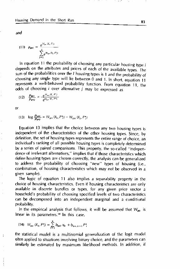
e'v, (11)
= amily
In equation lithe probability of choosing any particular housing type idepends on the attributes and prices of each of the available types. Thesum of the probabilities over the I housing types is 1 and the probability of choosing any single type will lie between 0 and 1. In short, equation 11even represents a well-behaved probability function. From equation ii, the
the odds of choosing i over alternative j may be expressednomic
as
- Pw ( P)
Pya (li, ,. P)
or su mer,
which log = Wi,,, (X,P) W.,, (X,P)
chastic Equation 13 implies that the choice between any two housing types is
s (y, a) independent of the characteristics of the other housing types. Since, by ability definition, the set of housing types represents the entire range of choice, an
individual's ranking of all possible housing types is completely determined by a series of paired comparisons. This property, the so-called "independence of irrelevant alternatives," implies that if those characteristics which define housing types are chosen correctly, the analysis can be generalized to address the probability of choosing "new" types of housing (i.e., combination, of housing characteristics which may not be observed in a
rticular given sample).
of all The logic of equation 11 also implies a separability property in the erits. If choice of housing characteristics. Even if housing characteristics are only
is available in discrete bundles or types, for any given price vector a household's probability of choosing specified levels of two characteristics
istically can be decomposed into an independent marginal and a conditional probability.
In the empirical analysis that follows, it will be assumed that W is
linear in its parameters.'0 In this case,
W,,,, (X1, P) = b,,,, , + P
the statistical model is a multinomial generalization of the logit model often applied to situations involving binary choice, and the parameters can similarly be estimated by maximum likelihood methods. In addition, if
84 John M. Quiglev
preferences can be approximated by any function linear in its parameters
McFadden has shown that the likelihood function is concave, implying that
iterative estimation procedures converge upon the unique maximum likeli
hood estimator of the b parameters.'1 Equations 13 and 14 imply the multinomial logistic model to be
estimated separately for each stratification of income and socioeconomic
Empirical estimates of the demand for housing types and individual housing characteristics are obtained by using information from a largescale home interview survey conducted in 1967 in the Pittsburgh Metropolitan Area.'2 The empirical analysis uses price and housing stock information gathered on some 25,000 dwelling units to analyze the housing choices made by approximately 3,000 rental households who made location decisions within the seven year period 1960-1967.
The central hypothesis is that the multiplicity of work places interacts with the location of durable stocks of differentiated housing types to create systematic variation in the relative prices of housing types that confront households in the urban area. These systematic variations in relative prices are derived from variations in journey-to-work costs, and by hypothesis they affect households' choices among housing types or housing configurations.
Besides testing this hypothesis in some detail, the analysis allows empiri. cal testing of several other hypotheses concerning housing market behavior. These hypotheses are developed following the definitions of the particular variables used in the analysis. The operational definitions of the types of residential housing, their component characteristics, and the calculation of the effective prices facing each household are first discussed in turn.
THE TYPES OF RESIDENTIAL HOUSING
As previous analyses have stressed, payment for housing services includes payments for a wide variety of qualitative and quantitative attributes of residential structures, In defining discrete housing types, or combinations of these underlying attributes, theoretical considerations suggest two rough guidelines. On the supply side, the existence of discrete housing types or submarkets implies that it must be costly to transform housing units among submarkets. On the demand side, housing units within any submarket must be viewed as (virtually) identical, but housing units in different submarkets must be viewed as separate and distinct entities.
y
SI
at
e
ic
al
et-ckhe
ho
cts
ate
ntes
S's
ra-
In-be-thethethesed
des
ofonsgh
s orongust
kets
85 Housing Demand in the Short Run
Both the empirical and theoretical literature suggest that households ofdiffering income and family size will choose units of varying residentialdensity (or lot size) and varying interior size. In addition, the qualitativecharacteristics of residential Structures are valued by households.
Based upon these considerations and available sample information 18types or submarkets of rental housing are defined by proxies for residentialdensity, quality, and interior size. Residential density (or effective lot size) isproxied by structure type, which is reported in three categories; singledetached units, common-wall units (including row and duplex houses),and multifamily (apartment) units. The age of the dwelling unit is used as a proxy for housing quality andobsolescence. Units are classified into two categories: those built before1930 and those built after 1930. The cutoff year for defining age categorieswas chosen from considerations of sample size with respect to the data
source. It should also be noted that there was relatively little new residential construction in the Pittsburgh metropolitan area during the period1930-1 945.
Although it would have been preferable to use floor space in describinginterior size, the only available information in the sample is the number ofbedrooms in each dwelling unit. Interior size is thus proxied by the numberof bedrooms in the unit, reported in three categories: less than two bedrooms, two bedrooms, and three or more bedrooms.
The types of rental housing are thus described by 1 8 combinations: threestructure types by two quality levels by three interior size measures.
The Effective Prices of Housing Types
For each of the 18 types of residential housing, the surface of contract prices (monthly rents) is estimated by the average price in each of 50 locations (zones) in the metropolitan area. The available stock of each type01 housing is similarly described by the number of units in each zone. Calculations made by households of the costs of commuting to work arefacilitated by reference to a set of 330 work sites (zones) and 130 residence sites (zones).
Thus from equation 1 the surface representing the total cost of consuming housing of type i is
To estimate the monthly cost of work trips we make two strong assump. tions. First, we assume that households are free to choose the number of hours they work; secondly, we assume that workers neither value the act of traveling nor the intrinsic characteristics of travel modes. These assump. tions imply that the time spent traveling is valued at the (marginal) wage rate and that the choice of mode is made solely on the basis of time and money costs.
Thus for an individual with (marginal) wage w, the monthly transpon costs (TC) from fixed work place Ito residence place m will be equal to the minimum of the cost of a single trip on public transit (TP,) or the cost of a trip by private auto (T%,) multiplied by the number of work trips per month (N); i.e.,
T, = N mm (TP,, TA)
The cost of trips by public transit is composed of out-of-pocket fares (F) and time costs. Let T'm be the elapsed time by public transit between work place j and residence site in.
TPjmw 'jm + Tm Wp
Similarly the cost of trips by private auto includes the out-of-pocket cost of fuel and maintenance'4 (expressed as E dollars per minute), the cost of parking at the destination (expressed as half the costs of all day parking at the work site, C) and the costs of time (where Tm is the interzonal travel time for an auto trip):
T, L + T (E + w)
The total expenditure required to consume housing type i at any residentiallocation m may be computed as
P = R., mm t(F, + Tm wy), + T,, [E + wJ)}
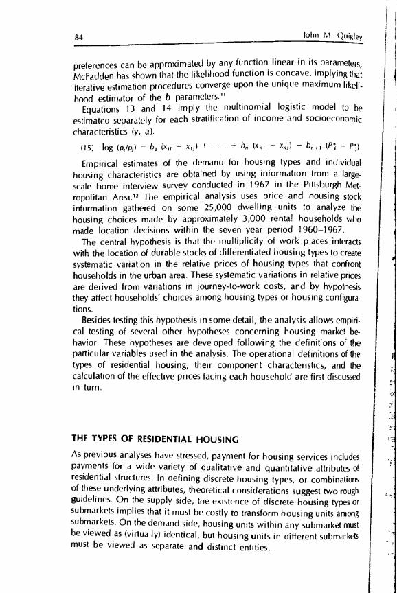
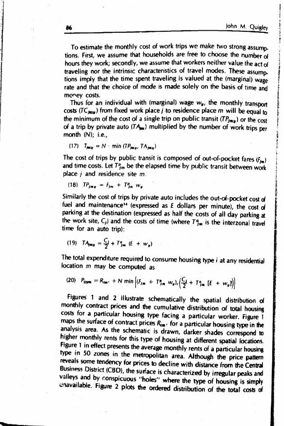
Figures 1 and 2 illustrate schematically the spatial distribution of monthly contract prices and the cumulative distribution of total housingcosts for a particular housing type facing a particular worker. Figure 1maps the surface of contract prices R._, for a particular housing type in theanalysis area. As the schematic is drawn, darker shades correspond tohigher monthly rents for this type of housing at different spatial locations.Figure 1 in effect presents the average monthly rents of a particular housingtype in 50 zones in the metropolitan area. Although the price patternreveals some tendency for prices to decline with distance from the CentralBusiness District (CBD), the surface is characterized by irregular peaks andvalleys and by conspicuous "holes" where the type of housing is simplyunavailable. Figure 2 plots the ordered distribution of the total costs of
p.of
of
p-
)rt
to
st
er
k
of
of
at
el
of
Is.
al
id
lyJf
FIGURE 1 Schematic of the Surface of Monthly Rents for New TwoBedroom CommonWaIl Units in thetan Study Pittsburgh Metropoli..
''22:1'.SIl77(f.,-,ff771) IIl)lI))IIlI III 1)) 222)) lIIllll)i)iij,,,,,,j,,, l))))));)) II)))111)2)2)1)1)
7'1175 llIl)flI,7, 111177777) I II))J)))j),p) I) 1I)1)))ll)li, II II III) I) I)) II Ill II
consuming this type of housing faced by an individual with wage rate of$7,000 employed in the CBD. The figure was plotted by applying equation20, using the three travel matrices, Firn, T,22, and T,,2 (130 x 330), and thevector of parking costs C3 (1 x 330) aggregated from the 1 967 Pittsburghsurvey.
If households possessed perfect information, the optimal residentiallocation for this type of housing for the individual represented in Figure 2and its effective price to him would be the actual minimum of thecumulative price distribution, $122 on the diagram.
Because housing market information is costly and because the individual estimates of total housing costs are subject to measurement error,the empirical analysis does not rely upon the single minimum total price asan estimate of the effective housing price facing an individual. Instead the average total price of the lowest five percent of the stock of each housingtype is used to estimate the effective price minimum. Figure 2 illustratesthis computation and shows an estimated minimum price of $128.
In addition to these price estimates, a variable measuring the totalnumber of units of each housing type available in the metropolitan area is
$
a
FIGURE 2 Ordered Distribution of Total Cost of Consuming New Tø Bedroom Common-Wall Units Facing a Household in the CBD With an Annual Income of $7,000
P,ykm
250
225
200
175
* plik
125
100
0 0 10 20 30 40 50 60 70 80
Per cent of the housing Stock
included. This additional measure is used to proxy for the information available to consumers about the location and prices of alternative housing types.
The Complete Model and Some Additional Hypotheses As stated and developed in previous sections, the model to be estimated inthis section is the multinornial logistic. For each cross-classification of income and family size, the logarithmic odds of the choice between anytwo types of residential housing is a linear function of the attributes of each housing type (in this case proxies for residential density, interior size,quality, and availdbility in the metropolitan area and the eftective price Oteach housing type (which may vary for particular households). Fromequation 15, the specific model is:
CW is a dummy variable with a value of I if j is a common-wall unitAPT1 is a dummy variable with a value of I if i is an apartment unitBR1 is the number of bedrooms in type IAGEI is a dummy variable with a value of 1 if I was built before 1930P is the effective monthly cost of consuming housing type i
and
ST, is the number of units of housing of type i in the sample
The parameters of equation 21 are estimated separately for each of 30 combinations of income and family size. Equation 21, together with theerror term assumption in equation 9, define the likelihood function (L)whose logarithm is:
log L = - jD1r log{ (CWkT - CW1r)r=1 t=I k=i
+ . + b6 (STkr ST1r)jJ
where
R is the sample size for each stratification of income and family sizeand r 1, 2.....R is the index of observations, andDir is a dummy variable with a value of 1 if the rth household chooses
housing type I.
Maximum likelihood estimates of the parameters of equation 22 areobtained by an iterative process. If this model of housing choice is appropriate, several hypotheses about the signs and magnitudes of the estimated parameters can be addressed. First, from equation 11 the ownprice elasticity of choice among housing types is
N1, = Pb5(1 - pi)
and the cross-price elasticity is
N. = Pb5p
To insure a negative own-price elasticity and a positive cross-price elasticity, the estimate of b, should be negative for each stratification of income and family size.
We should also expect the parameter b4 to be negative since, ceteris paribus, households prefer higher quality dwelling units, that is, holding structure type and size constant, housing types indexed by quality form a "commodity hierarchy." Similarly, holding structure type and quality
e
90 John M. Quiley
constant, housing types indexed by size form a "commodity hierarchy"; thus we expect the estimate of b to he positive. The coefficient of the housing stock term, b6, should be positive, since households can obtain more information, at the same search cost, for housing types in greater
supply. Holding income constant, we should expect that larger families demand
larger units and more exterior space. Thus for larger families with the same income we should expect that the estimate of b3 will be larger than for small families. Similarly, the estimates for b, and b2 should be smaller in magnitude (or more negative) for larger families than for smaller famjlips
Holding family size constant, we expect that higher incomes are associated with greater consumption of higher quality, larger units with more exterior space. Thus for the same family size we expect that the estimate of b3 will be larger for the higher income households than for lower income households. Similarly, the estimates of b1, b2 and b4 should be more negative for higher income households than for lower income households.
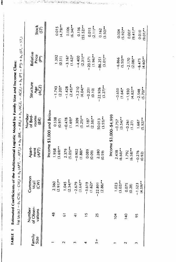
Table presents the coefficients of the multinornial logistic model,1
estimated by the maximum likelihood method, for each of thirty combinations of income and family size. The model is estimated separately for each of five family sizes (corresponding to households of 1, 2, 3, 4, and 5 or more members) for each of six income classes (corresponding to annual incomes of less than $3,000$4,999, $5,000$6,999, $7,000$9,999, $10,000$14,999, and $15,000 or more).
For each household in the sample, the total cost was calculated for each of the 18 types of residential housing at each possible location by using equation 20 and the mid-points of the income classes to derive hourly wage estimate w;'5 the minimum total cost (P) including housing and transport cost, was estimated for each housing type by calculating the average price of the cheapest 5 percent of the stock for each household. One type of residential housing was chosen as a numeraire; the prices facing each household are relative to this numeraire.'6
For each of the 30 nonlinear regressions, the results reported in Table 1 were obtained by specifying a convergency criterion of .01. In most cases five or six iterations were required. For each set of results the sample size is noted and the asymptotic t ratios of the coefficients appear in parentheses.
In 26 of the 30 equations the relative price coefficient has the anticipated sign; the estimated coefficient exceeds its standard error in 22 equations and it appears highly significant in 16 stratifications. The ratios of the relative price coefficients are substantially lower for the two higher income groups. For renter households earning between $10,000 and $15,000 a year, three of the estimates coefficients are significant at about the .05 level and the other two are insignificant. For renter households earning more than $15,000 a year, none of the price coefficients aresignificant.
TA
BLE
1
Est
imat
ed C
oeffi
cien
ts o
f the
Mul
tinom
ial
Logi
stic
Mod
el b
y F
amily
Siz
e an
d In
com
e C
lass
: lo
g (p
,/p.)
= b
1 (C
W1
- C
Vv)
+ h
2 (A
PT
1 -
AP
T,)
+ b
3 (B
R -
BR
,) +
b4
(AC
E1
- A
CE
,) +
b (
P
- P
) +
b6
(ST
e -
ST
,)
Num
ber
Num
ber
Com
mon
A
part
of
Bed
-S
truc
ture
R
elat
ive
Fam
ily
of O
bser
-W
all
men
t ro
oms
Age
P
rice
Sto
ckS
ize
vatio
ns
(CW
) (A
PT
) (B
R)
(AC
E)
(P*)
(S
T)
Inco
me
$3,0
00 a
nd B
elow
48
2.
560
1 .9
58
0.53
8 -1
.743
1.
392
0.0
15(2
.91)
**
(3.6
9)**
(0
.97)
(2
.20)
* (4
,79)
**(0
.51)
61
1
.045
2.
379
-0.4
78
-1.4
28
-3.1
67
0.00
6(2
.34)
**
(5.0
5)
(1 .6
9)*
(2.4
5)**
(1
.62)
(6
,34)
**
3 41
-2
.679
-0
.902
3.
309
-3.2
10
-4.4
00
0.13
6(3
.64)
**
(1 .8
8)*
(5.2
5)**
(4
.04)
* (2
.3 1
) **
(5
5.52
)**
4 15
-3
.619
0.
089
5.18
7 -0
.201
-2
0.57
1 0.
015
(1 .6
2)*
(0.0
9)
(2,3
8)**
(0
.10)
(1
.96)
* (2
.1 1
)**
5+
25
-22.
89 1
2.
280
50.0
13
-22.
926
-86.
251
0.16
2(2
.86)
* (0
.59)
(3
,55)
**
(3 .2
7)*
* (3
,01)
**
(3.5
0)*
Inco
me
$3,0
00-$
4,99
9 1
1.02
310
4 2.
438
-0.7
57
-0.6
50
-6.8
66(3
.02)
**
(6.6
8)*
0.00
4 (3
.54)
(1
.64)
(5
.50)
**
(5.9
2)*
2 14
0 0.
075
1.79
2 -0
.261
-1
.930
-2
.170
0.
007
(0.2
8)
(6.5
8)**
(1
.27)
(4
.82)
(2
.08)
**
(9.4
1)'
95
-1.5
23
-0.2
76
1,68
73
-2,5
48
-6.4
75(4
59)*
0.
010
(0.9
2)
(5.9
2)**
(5
.70)
**
(4.6
0)
(9.0
1)
0
'-fl.
Saa
*a
TA
BLE
1
(con
tinue
d)
Num
ber
Num
ber
Com
mon
A
part
-of
Bed
-S
truc
ture
R
elat
ive
Fam
ily
of O
bser
-W
all
men
t ro
oms
Age
P
rice
Sto
ckS
ize
vatio
ns
(CW
) (A
PT
) (B
R)
(AG
E)
(P1)
(S
T)
4 88
-1
,054
-0
,810
1.
770
0.45
5 -6
.364
0.
006
(3.0
0)1*
(2
.40)
1*
(5.2
0)"
(1 .2
0)
(3.8
7)"
(593
)**
5+
87
-1.2
78
-1.9
30
3.28
2 -0
.247
-3
.998
0.
010
(3.7
2)"
(4.3
4)1*
(8
.91)
1*
(0.6
7)
(2.9
0)"
(9.1
5)"
Inco
me
$5,0
00-$
6,99
9 1
91
0.15
0 2.
564
-1.2
22
-3.0
49
-1.8
88
0,00
9(0
.31)
(5
.50)
1*
(3.2
1)"
(4.2
6)"
(1.2
0)
(654
)1*
2 22
3 0.
291
0.87
4 -0
.223
-0
.223
-2
.906
0.
003
(1.6
5)*
(4.2
9)1*
(5
.1 3
)1*
(1.2
5)
(3.9
8)"
(7.7
9)"
3 22
4 -1
.500
-0
.849
2.
020
-2.3
83
-4.4
65
0.01
0(7
.06)
" (4
45)1
(1
0.92
)1*
(9.0
3)1*
(5
.87)
" (1
4.89
)"
4 19
4 -2
.693
-0
.903
3.
823
-2.7
38
-4.1
40
0.01
4(1
0.1
2)"
(4.2
3)1*
(1
3 .5
4)1
* (8
.86)
" (4
.91)
" (1
4.16
)"5+
22
3 -1
.591
-2
.0 1
3 3.
170
-0.8
93
-6.1
16
0.00
8(7
53)1
* (7
.32)
1*
(13.
46)1
* (3
,89)
**
(6.6
1)"
(12.
16)*
*
Inco
me
$7,0
00.-
$9,9
99
79
0.66
41
1.56
1 -0
.586
-3
.179
-0
.491
0.
006
(1.5
5)
(3.7
3)
(2.3
9)
(6.1
1)"
(0.4
4)
(5,5
4)1
C,.
2 22
8 0.
196
0.35
0 0.
479
-1.8
81
-1.4
03
0.00
6(0
.87)
(1
.65)
* (3
39)*
* (7
.81
) (2
.26)
" (1
1.67
)"3
218
-1.2
42
-0.4
90
2.27
2 -2
.955
-3
.490
0.
010
(543
)**
(2.3
7)"
(11
.92)
* (1
0.95
)**
(495
)**
(14.
24)"
4 16
6 -2
.340
-0
.616
4.
193
-4.3
04
-3.5
65
0.01
5(9
.1 8
)**
(1 .8
5)**
(1
1 .7
0)**
(3
54)*
*(9
.63)
" (1
2.50
)"5+
17
3 -2
.096
-1
.561
4.
159
-0.7
50
-5.0
35
0.00
9(8
.46)
**
(5,1
7)*
* (1
2.1
2)**
(3
.00)
" (4
.90)
**
(11.
82)"
Inco
me
$1 0
,000
-s 1
4,99
9
24
-'1.2
67
-1.7
36
0.49
31
-4.6
51
1.10
5 0.
020
(0.9
2)
(1.1
6)
(0.6
8)
(2.9
2)"
(0.2
2)
(3.4
4)"
2 15
3 -0
.108
0.
391
0.06
0 -1
.503
-1
.262
0.
003
(0.4
0)
(1.5
1)
(0.4
4)
(6.4
6)"
(1 .8
3)*
(6.5
9)"
3 83
-0
.640
-0
.284
1.
368
-1.0
51
-1.7
11
0.00
4(1
99)
* (0
.82)
(5
.72)
" (3
.25)
" (1
.81)
(5
.52)
" 4
56
-2.5
66
2.13
4 7.
477
-6.3
66
-2.0
31
0.02
3(4
.63)
" (2
.72)
" (6
.89)
" (5
.49)
" (1
.10)
(6
.94)
"5+
67
-2
.511
-3
.769
4.
743
-2.6
74
-3.3
48
0.01
0(5
.78)
" (4
.40)
" (7
.39)
" (4
,99)
" (1
.76)
(6
.20)
"
Inco
me
$15,
000
and
Abo
ve
17
-19.
346
-10.
694
1.25
6
-3.6
86
-3.3
21
0.04
0 (0
.03)
(0
.02)
(0
.01)
(0
.01)
(0
.00)
(0
.03)
TA
BLE
1
(con
clud
ed)
Num
ber
Num
ber
Com
mon
A
part
-F
amily
of
Obs
er-
of B
ed-
Str
uctu
re
Rel
ativ
eW
all
men
t ro
oms
Age
Siz
e va
tions
(C
W)
Pric
e S
tock
(AP
T)
(BR
) (A
GE
) (P
*)
(ST
) 2
50
-1.6
56
-0.2
30
1.92
6 -3
.534
0.
084
0.01
1(2
.31)
**
(0.4
7)
(4.2
8)**
(5
.48)
" (0
.06)
(5
,68)
**
3 24
-3
.605
1.
531
3.46
6 -0
.093
-1
.572
(345
)**
0.00
0(1
.15)
(4
.21)
" (0
.11)
(0
.63)
(0
.00)
4 14
-2
.324
-1
.390
3.
347
-3.4
46
-2.4
58
0.01
2(2
.1 0
)*t
(1.3
2)
(3.3
Ø)*
(2
.46)
(0
.79)
(2
.77)
"5+
10
-0
.251
9.
609
13 .0
27
-0.8
67
2.34
3 0.
002
(0.1
3)
(0.0
9)
(0.1
2)
(0.5
0)
(0.2
1)
(0.3
1)
NO
TE
: A
sym
ptot
ic t
ratio
s in
par
enth
eses
. "in
dcat
es c
oeffi
cien
t diff
eren
t fro
m z
ero
at .0
1 le
vel,
indi
cate
s co
effic
ient
diff
eren
t fro
m
zero
at .
05 le
vel.
95 Housing Demand in the Short Run
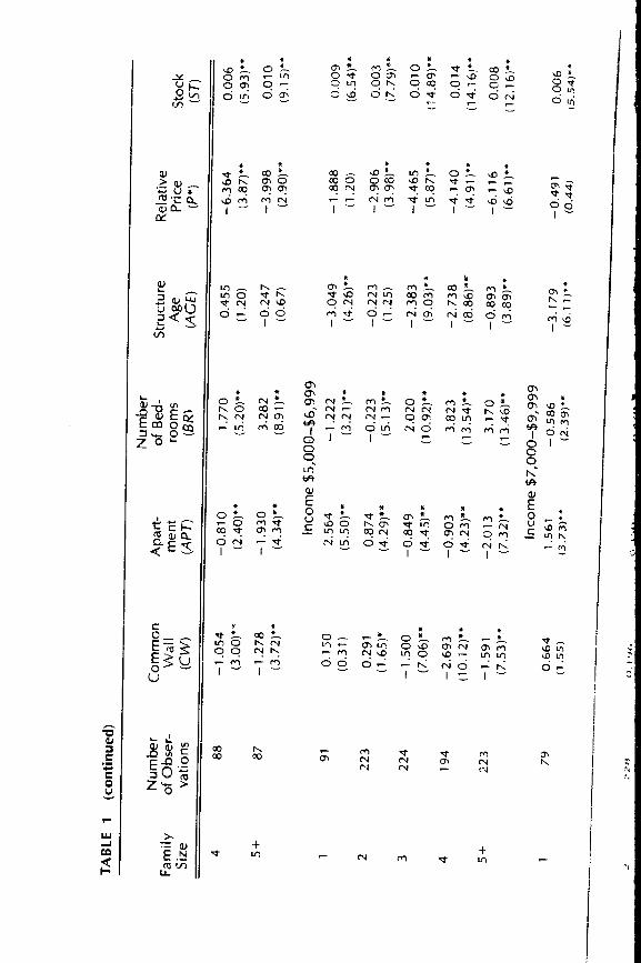
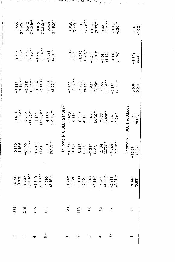
The patterns of significance suggest that the choices of housing types forthe overwhelming proportion of rental households (i.e. those lower andmiddle income rental households that, for this sample, comprise 85percent of the rental market), are strongly influenced by relative prices. Thetable also suggests a clear pattern in the magnitude of the relative pricecoefficients for families of different sizes. Within each income class, themagnitude of the price coefficient increases with family size. largerfamilies with greater demands for necessities are more responsive torelative prices in their choices among housing types. The estimated coefficient of the structure age variable has the anticipatedsign in 29 of the 30 equations and is highly Significant in 22 of the
stratifications. Again, the t ratios suggest that renters in the highest incomeclass are least Sensitive to structure age, but there does not seem to be astrong pattern in the magnitudes of the estimated coefficients acrossincome classes and family sizes. The coefficients of the number of bedrooffis indicate a systematic pattern
across income classes and family sizes. The coefficients are statisticallysignificant with the correct sign in 1 9 of the stratifications. For each of thesix income classes, the magnitude of the coefficient on the bedroom variable increases with family size. There is also a tendency for thecoefficient to increase with income level for a given family size.
The coefficient of the variable for commonwall units is statisticallysignificant in 20 of the 30 equations; the coefficient of the variable representing apartment units is significant in 15 stratifications. The patternof coefficients suggests, ceteris paribus, that single detached units arepreferred to either of these types of families with three or more members. Holding family size constant, the coefficients also indicate that singledetached rental units are preferred by those of higher incomes.
In general, the model performs less well for renters of the highest income class, those earning more than $15,000 a year. In part, this may be a reflection of the smaller sample sizes for households in this category. However, the results may also suggest that the definitions of the housing types are inadequate to model the behavior of the highest income group; the aspects of housing which motivate the residential location and housing choices of the highest income households are not well represented by only 18 types of residential housing.
Tables 2 and 3 illustrate the differences in housing consumption attributable, ceteris paribus, to variations in the socioeconomic characteristics of households. The tables indicate the predicted probabilities of consuming several housing characteristics using the coefficients of Table 1 and assuming each household in the metropolitan area faced the same effective housing prices (P). These probability estimates may be interpreted as those observed under the monocentric or equilibrium assumptions of the
Predicted Probabilities of Housing Type Choice, p,1,,TAULE 2 for Selected Incomes Across Family Sizes:
=
where
I'J = h,, !i ,
Family Size 1Type of Dwelling 2 4
Income $3000 -$4,999
Common-'alI units .11 .11 .39 .69 Apartments .84 .82 .38 .27 .06 Single detached .04 .07 .25 .34 .25 One bedroom .78 .79 .35 .12 .o Two bedrooms .20 .20 .53 .42 .48 Three bedrooms .02 .01 .12 .46 .49
Income $5,000-$6,999 Common-wall units .03 .22 .54 .52 .52 Apartments .94 .60 .23 .11 .oa Single detached .02 .17 .24 .37 .40 One bedroom .95 .66 .23 .10 .03 Two bedrooms .05 .28 .33.61 .61 Three bedrooms .00 .06 .16 .29 .64
classical theory. If all households were employed at a single work site they would, of course, face identical effective prices for the same type of residentia! housing.17 The probability estimates were obtained by substitution into equations 11 and 14 and by then forming the marginal totals.
Table 2 illustrates the probabilities for two income classes over the five family size categories. The table indicates that, as family size increases, households are less likely to choose multifamily units and are more likely to choose common-wall units and single detached units, For income levels of $3,000 to $5,000, the probability of choosing apartment dwellings declines from .84 for one-person households to .06 for five-person households; the probability of choosing common-wall units increases from .1 Ito .69. Similarly the probability of choosing single detached units increasesfrom .04 to .25 as family size increases from one to five members.
For a higher level of income, the table indicates (hat larger family sizes also systematically choose less dense housing configurations. In contrast tothe lower income group, households earning between $5,000 to $7,000have higher probabilities of consuming larger effective lot sizes at each
TABLE 3 Predicted Probabilities of Housing Type Choice, p,for Selected Family Sizes Across Income Classes.
where
W11,(X1, P) = b,,1 + I
Less than $3,000 $5,000- 7 flflfl-TypeolDwelling $3,000 $4999 $6,g9 $9,999 $14,999 $15,000+
family size. Holding family size constant, higher income householdssystematically choose less dense types of residential housing.
Within each income class, Table 2 indicates that increased family size isassociated with the choice of housing types with larger interior sizes (asmeasured by numbers of bedrooms). However, the comparison for the twoincome classes reveals that at the same family size, higher income households are generally more likely to choose two and three bedroom unitsthan lower income households.
Table 3 illustrates the differences in housing consumption across the six income classes for two stratifications of family size. The table indicates thatfor three-person families, the probabilities of consuming units with largerinteriors are very similar for households earning less than $7,000 a year.(The predicted average numbers of bedrooms are 2.0, 1.8, 1.9 and 2.0, respectively for the lowest four income classes.) Only for the two highestincome classes, where the predicted average number of bedrooms increases to 2.3 and 3.0 respectively, does higher income increase thelikelihood of choosing housing types with larger interior sizes.
rev
mc
cho
cbs
with
sjn1i
unit
there
fli
98 JohnM. Quigley
In contrast, for larger families the probability of choosing larger Units
increases systematicafly with income level. As income rises from $3,000 to$15,000 a year the probability of choosing a three bedroom unit
increasesfrom .00 to .97. The predicted average number of bedrooms for the sir income classes are 1.0, 2.5, 2.6, 2.7, 2.8, and 3.0 respectively.
For smaller families, the differences in the predicted Probability ofchoosing different structure types do not vary systematically with income. For larger families, however, the estimates in Table 3 suggest that increases in income are associated with higher probabilities of choosing singledetached units. The predicted probability of choosing single detached units increases from .00 to .50 as family income rises from $3,000 to $15,000 a year.
As has been emphasized throughout this discussion, the variation in the effective prices (Pt) facing different households arises from the interaction of contract housing prices and the accessibility costs to the specific work sites of different households. Within the sample, substantial variation existsin the effective prices facing otherwise identical households. By way ofillustration, Figure 3 presents the frequency distribution of the effective prices (P*) facing households of a single income class for two housing types. The figure indicates the effective prices relative to the numeraireused in the empirical analysis. The variation in the prices faced byindividual households arises because the spatial location of the minimumprice and its magnitude varies with work site, the transport network, andthe surface of contract prices.
To indicate the importance of these price differences in affecting thechoice of housing types, we have used the equations estimated in Table 1to calculate the predicted probabilities of choice among the housing typesfor otherwise identical households which are employed at four specificwork places iii the metropolitan area. One of these work sites is located inthe heart of the Pittsburgh CBD; a second is located iii the inner city, eastof the CBD; a third is located on the outskirts of the central city, and afourth is located in the suburbs east of Pittsburgh. Table 4 presents thepredicted probabilities of choice for households of the same income andfamily size who face the effective prices calculated for these four worksites. The predicted probabilities of choice for four-person householdsearning between $5,000 to $7,000 a year and employed at the four worksites are presented in the first section of Table 4. The predicted probabilities for a five-person household earning income in the same range andemployed at the same locations are presented in the second section. In thethird section of the table the probabilities predicted for a five-personhousehold of a lower income class are indicated.
The table clearly shows the differences in the consumption of housingattributes which arise from the variations in relative prices. For households
FIGURE 3 Frequency Distribution of Relative Prices for Two lypesof Housing Facing Households Earning Less Than $3,000a Year
25
Effective price of old,I bedroom common wall units
20
Effective price of old, r---i3 bedroom common wall units
-III
r_-hI_______o L___ 0.6 07 .8 0.9 1.0
IU 1.2 1.3 1.4 1.5Relative price, P
NOTE: Both prices are relative to the effective price of new one bedroom, commonwall units.
earning between $5,000 to $7,000 a year, the probability of choosing apartments declines systematically for four-person households whose work place is more distant from the Central Business District. Similarly, the probability of choosing single detached housing types increases systematically for tour-person households with less central work places. For fiveperson households. The same regular pattern of structure-type choices is revealed for the four work places. For larger households at the same income, however, those employed at noncentral places are more likely to choose larger effective lot sizes than smaller households.
For five-person households of a lower income class, the probability of choosing single detached housing increases with less central employment locations, but the probabilities are substantially lower than for households with larger incomes. The probability of choosing common-wall units similarly declines at noncentral employment sites, hut the probabilities are uniformly higher than for households with larger incomes.
Even at the same family size, variations in the effective prices affect households' choices of the interior size of units. For four-person families, there is a small but systematic increase in the probability of choosing housing types with more bedrooms at less central work sites. For fiveperson households of both income classes this tendency is more pronounced.
TABLE 4 Predicted Probabilities of Housing Type Choice, for Otherwise Identical Households at Four Work Sites
Work Places Inner Central
Type of Dwelling CBD City City Suburbs
Four-person Families--Income $5000-$6 999 Common-wall units .51 .54 .50 .42 Apartments .40 .29 .19 .11 Single detached .09 .17 .30 47 Onebedroom .16 .13 .13 .14 Two bedrooms .63 .63 .61 Three bedrooms .21 .23 .26 .28
Table 4 clearly shows how variations in the intrametropolitan costs ofconfigurations of residential housing affect households' choices of consuming several attributes of the residential housing "bundle".
The theory of the housing market and the computation of the effectiveprices of housing units used in the empirical analysis suggest that theseprice variations arise because: existing housing units are costly to transformand the spatial distribution of housing types changes slowly in response tomarket forces; households employed at different sites face different accessibility costs to the available supplies of durable housing units. By neglecting these considerations
many analyses of household location and demand for "housing" have overlooked a crucial link in understanding whyhouseholds choose particular spatial locations and why households choosecomponents of the bund!e of housing services.
101 Housing Demand in the Short Run
NOTES
Aggregate studies whi&h neglect housing prices in focusing on uic.ome expendituresinclude: Margaret Reid, Housing and Income (Chicago: Universits of Chicago Press1962); Alan R. \'\'inger, 'Housing and Income,"
pp. 226-232. Muth's study includes an index ofWestern Economic Journal June 1968, construction costs (tliacross cities, and de Leeuw's intercity analysis Boeckh index) uses the Bureau of Labor Stjjk-5city-worker budget to provide an average price for a 'standard" bundle of housingservices. See Richard F. Moth, "The Demand for
Non-farm Housing," in The Demandfor Durable Goods, Arnold C. Harberger, ed. (Chicago: University of Chicago Press,1962); Frank do Leeuw and Nkanta F. Ekanern, "The Demand for Housing: A Reviexx' ofthe Cross-Section Evidence," Review of Economics and Statistics, February 1971, pp.1-10.
See Mah!on R. Siraszheim, "Estimation of the Demand for Urban Housing Services fromHousehold Interview Dat,i," Revieis of Economics and Statistics February i pp.1-8; Mahlon R. Straszheim, An Econometric Analysis of the Urban Housing Market(New York: National Bureau of Economic Research, 1975); John F, Kain and John M.Quiglev, Housing Markets ann Racial Discrimination: A MicIOcConornic Analysis (NewYork: National Bureau of Economic Research, 1975); John M. Quigey, "Racial Discrinhination and the Housing Consumption of Black Households," in Patterns of RacialLjiscrirriin,stion Vol. 1: Housing, George M. Von Furstenberg ed. (Lexington, Mass.:D.C. Heath, 1974); A. Thomas King, "Households in Housing Markets' The Demand forHousing Components" (College Park, Md.: Bureau of Business and Economic Research,University of Maryland, 1973).
The classic references include: Richard F. Muth, Cities and Horning (Chicago: University of Chicago Press, 1969); Lowdon Wingo, Transportation and Urban Land(Washington, DC,: Resources for the Future, 1961); William Alonso, Location and LandUse (Cambridge: Harvard University Press, 1964). James L. Ssveeney, "Quality, Commodity, Hierarchies, and Housing Markets," StanfordUniversity, Department of Engineering.Economic Systems, mimeographed, October1972.
These estimates of the implicit prices of housing attributes are derived from Lancaster's analysis of hedonic goods. See Kelvin J. Lancaster, "A New Approach to ConsumerTheory," Journal of Political Economy, April 1966, PP 132-156; Sherwin Rosen,"Hedonic Prices and Implicit Markets: Product Differentiation in Pure Competition,"Journal of Political Economy, January/February 1974, pp. 34-55. For a recent survey ofthis literatwe as related to housing markets see Michael J. Ball, "Recent Empirical Work on the Determinants of Relative House Prices," Urban Studies, June 1973, PF) 213-233.John F. Kain, "The Journey to Woik as a Determinant of Residential Location," Papers and Proceedings of the Regional Science Association 1962, pp. 137-161.
7. It may he that the! types of residential housing form a "hierarchy" in the sense definedby Sweeney, i.e. that
(NI) UX11, z0) > U(X, z0)
tor all coilsurners. More generally, since x is multidimensional, it is likely that only some housing types are strictly hierarchical. For example, it the components of x include "housing quality" and "size," it may be true that all consumers prefer higher quality to lower quality units and larger dwelling units to smaller units; consumers may have mixed preferences, however, regarding the tradeoff between larger, lower quality units and smaller, higher quality units.
a
I
'5
.5'
102 Iohn M. Quiglc'y
ft H. Bluch arid 1. Marschak, ''Randwii Ordeiines and Stodistiu 11 Rvsponc"(ontribut,n to Probabtht', and Stati.stiis, I. 01km. ed. (St,inlnrd: Stanford UniversityPress, 1960).
Daniel McFadden. 'The Revealed Preferences of ,i Government Bureaucracy" 1'echq. cal Report W. 17, Institute of International Studies, University of
California_Berkrlt.sNovember 1968; Charles River Associates, "A Disaggregated Behavioral Model of Urban Travel Demand," Report CRA-156-2, March 1972; Daniel McFadden "Conch. tional LogO Analysis of Qualitative Choice Behavior,'' in Frontiers in F(oflorne(rjCsZaremka, ed. (New York: Academic Press, 1974).
p.
Although this assumption (as well as (he assumed error term distribution in equation 9) is made solely in the interest of tractability, it is not quite as restrictive as it may appear, since a wide variety of functional forms may, in principle, be accommodated by dummyvariabies ad piecewise linear approximations.
11 McFadden, 1968 (sec note 9). Details concerning the survey instruments and the underlying data may be found in JohnM. Quigley, "Residential Location with Multiple Workplaces and a IIeterugenc'ous Housing Stock," Discussion Paper Numbe, 80, Program on Regirniat ,mrt UrbanEconomics, Harvard U niversity, September 1972. For evidence on the relationship between housing age and "objective nhc'asur' ofhousing quality," see John F. lOin and John M. Quigley, "Evaluating the Quality of theResidential Environment" Lnvironrrrent and P!annin, Vol. 2, 1970, p. 21-32 Cost estimates were obtained from John B. Lansing aiid G. Hendricks, "How PeoplePerceive the Cost of the Journey to Work," No. 197, Highway Research Board, 1967,Pp. 44-55. For the six income classes the (assumed) midpoints and the associated hourly wages(based upon a 40 hour week for 50 weeks per year) are:
Although the methodology can be briefly stated, the calculation of the effective pricesinvolved estimating the entire surface of total housing costs lacing each household foreach type of housing and "scanning" each surface to find the average price of thecheapest fise percent of the stock of each type. For each household, its work place andincome class thence an estimate of its wage rate) are sufficient to calculate theaccessibility cost of each residential location. Knowledge of this cost plus the estimate ofcontract prices at each residential location for each housing type allowed a surface oftotal housing Costs to be defined for each type of housing. For each type of housing, theprices and the number of units at each residential location were scanned to estimate theaverage total cost of the cheapest five
percent of the stock when viewed from the workplace of each household at its wage rate. The price of one bedroom common.wall unitsbuilt after 1930 was used as the numerajre Alternatively, if several work places existed and the markets for each type of residentialhousing were in equilibrium, differences in the effective prices facing similar householdscould arise only if wages for identical labor inputs varied by ss'ork place.