Lauren Parker & Wei Ying| MUSA 507 | HW 5 P a g e | 1

LAUREN PARKER & WEI YING

MUSA 507: MIDTERM

Due: Oct. 17, 2014

1 Introduction

The purpose of this project is to develop a regression model that can accurately predict home sale prices at multiple

locations within Philadelphia. Property is a significant part of economy as well as relevant to city planning; as such,

housing market prediction has a great impact on housing trade and economic development. Accordingly, accurate

predictions of housing prices is a vital task, to which we should focus much attention.

However, making accurate predictions is anything but an easy work, for the variability of actual home prices is affected

by many factors. Therefore, the first challenge of this project is to determine what factors are related to home price by

referring to housing articles and by testing candidate variables correlation to the home prices. Additionally, the

accuracy of prediction depends on the regression model we build, but linear regressions are a somewhat simple

approximation of reality and can fail to explain the exact relationship between independent variables and the

dependent variable. Therefore, finding variables that are highly related to home prices is an important, yet difficult task

for a good linear regression model.

Our overall modeling strategy is building and improving a regression model using data of training sites, or observations

for which we have home sale prices, and then using our best model to predict sales fo a test dataset, or sites for

which we have no sale price. We set existing home prices of training sites as the dependent variable and compile several

explanatory factors as independent variables. We check the relationship between each independent variable and home

prices in order to make log transformations when necessary and remove outliers to improve the model. We then test

the regression model within the training data and judge the residual error between actual values and predicted values.

We included 12 variables in the final regression. The adjusted R2 of our model in training samples is 0.56, which suggests

a relatively explanatory regression. In our out of sample testing, we got a R2 as 0.5624, and the root mean square error

(RMSE) of 0.8533, which is generally a strong model. Overall, we believe the regression model to be a fairly reliable way

to predict home prices in Philadelphia.

2 Methodology

Data Collection and Processing

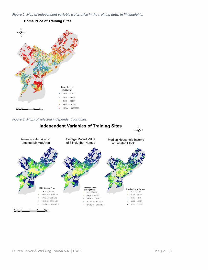
In addition to the data originally provided by Ken Steif, we tried to find other possible variables that may explain home

prices. Figure 1 presents all of our original candidate variables, data sources and processing steps. In total, we tested 44

variables to determine which were best at improving the explanatory power of the model. We also present maps of our

dependent variable (Figure 2) and several key independent variables (Figure 3).

Figure 1. Table of all variables tested for explanatory power.

Varia le Des riptio Data Sour e Pro essi g

Ke _ID U i ue ID Ke “teif

SalePri e Depe de t Va ia les sale i dolla s Ke “teif

SaleMo th Mo th of the ea i of sale Ke “teif

Fro tage idth of pa el Ke “teif

Depth le gth of pa el Ke “teif

GarageDu Whethe o tai ga age Ke “teif

E tCo d Catego i al a ia le des i i g o ditio of uildi g e te io

Ke “teif

Lauren Parker & Wei Ying| MUSA 507 | HW 5 P a g e | 2

Varia le Des riptio Data Sour e Pro essi g

YearBuilt ea of o st u tio Ke “teif

Nu Roo s Nu e of oo s Ke “teif

Nu BedR s Nu e of ed oo s Ke “teif

Nu Baths Nu e of aths Ke “teif

TotLi Area Total i te al s ua e footage Ke “teif

Pop Populatio i i lo k g oup of house poi t. Ce sus Bu eau, A GI“: spatial joi losest pol go

MedI Media household i o e of lo k g oup of house. A e i a Co u it “u e , -

A GI“: spatial joi losest pol go

White Nu e of hite households i lo k g oup of house. Ce sus Bu eau, A GI“: spatial joi losest pol go

AfA Nu e of Af i a -A e i a households i lo k g oup of house.

Ce sus Bu eau, A GI“: spatial joi losest pol go

A I Nu e of A e i a I dia households i lo k g oup of house.

Ce sus Bu eau, A GI“: spatial joi losest pol go

Asia Nu e of Asia households i lo k g oup of house. Ce sus Bu eau, A GI“: spatial joi losest pol go

HiPI Nu e of Ha aiia a d Pa ifi Isla de households i lo k g oup of house.

Ce sus Bu eau, A GI“: spatial joi losest pol go

Other Nu e of households of "Othe " a e i lo k g oup of house.

Ce sus Bu eau, A GI“: spatial joi losest pol go

T oRa e Nu e of households of "T o ‘a es" i lo k g oup of house.

Ce sus Bu eau, A GI“: spatial joi losest pol go

HH Nu e of households i lo k g oup. Ce sus Bu eau, A GI“: spatial joi losest pol go

O HH Nu e of o upied households i lo k g oup. Ce sus Bu eau, A GI“: spatial joi losest pol go

Va HH Nu e of a a t households i lo k g oup. Ce sus Bu eau, A GI“: spatial joi losest pol go

P tWhite Pe e t White households i lo k g oup. Ce sus Bu eau, A GI“: spatial joi losest pol go

A eTa MktVal A e age a ket alue of houses ea est to Ke 's house.

Cit of Phila. Offi e of P ope t Assess e t

A GI“: Ge e ate Nea Ta le tool; ge e ate a e age a ket alue of eigh o houses

S hDistFt Dista e ft to losest s hool. PA“DA A GI“: spatial joi losest poi t

BusDistFt Dista e ft to losest us stop. DV‘PC A GI“: spatial joi losest poi t

StrDistFt Dista e ft to losest st eet i te se tio . DV‘PC A GI“: spatial joi losest pol go

ParkDis Dista e ft to losest pa k poi t Ope Data Phill A GI“: spatial joi losest pol li e

HealthDis Dista e ft to losest health e te Ope Data Phill A GI“: spatial joi losest poi t

Re reaDis Dista e ft to losest e eatio pla e Ope Data Phill A GI“: spatial joi losest poi t

A eSalePrKe Near A e age sale p i e of houses ea est Ke 's house. Ke “teif A GI“: Ge e ate Nea Ta le tool

E pP tLa or E plo e t ate i hole la o fo e i e sus t a t of house poi t

A e i a Co u it “u e Cal ulate the pe e tage

E pP tTotal E plo e t ate i total populatio i e sus t a t of house poi t

A e i a Co u it “u e Cal ulate the pe e tage

GMAA ePri e A e age sale p i e of Ke 's houses ithi ea h Geog aphi Ma ket A ea GMA .

Ope Data Phill A GI“: spatial joi a e age

Ce terCit Dis Dista e ft to Philadelphia e te it Ope Data Phill A GI“: spatial joi losest pol go

ParkPolDis Dista e ft to losest pa k pol go Ope Data Phill A GI“: spatial joi losest pol go

Co erDis Dista e ft to losest o e ial zo e Ope Data Phill A GI“: spatial joi losest pol go

I dusDis Dista e ft to losest i dust zo e Ope Data Phill A GI“: spatial joi losest pol go

WaterDis Dista e ft to losest h d olog pol go Ope Data Phill A GI“: spatial joi losest pol go

Parki gDis Dista e ft to losest pa ki g lot Ope Data Phill A GI“: spatial joi losest poi t

ParkNo Nu e of pa ks ithi . - ile uffe of house poi t Ope Data Phill A GI“: uffe ; spatial joi ou t

Re reNo Nu e of e eatio pla es ithi . - ile uffe of house poi t

Ope Data Phill A GI“: uffe ; spatial joi ou t

Parki gNo Nu e of pa ki g lots ithi . - ile uffe of house poi t

Ope Data Phill A GI“: uffe ; spatial joi ou t

Distri ts_I de Du : if Ke 's house as i of dist i ts. “et as fi ed a ia les e.g.Dist i t_

Ope Data Phill A GI“: spatial joi poi t falls i side

Co ditio _I de Du a ia le i di ati g o ditio of uildi g e te io e.g. HighCo d

Ke “teif Mask sites o ditio as High o ditio , Mediu Co ditio o Lo o ditio

Lauren Parker & Wei Ying| MUSA 507 | HW 5 P a g e | 3

Figure 2. Map of independent variable (sales price in the training data) in Philadelphia.

Figure 3. Maps of selected independent variables.

Lauren Parker & Wei Ying| MUSA 507 | HW 5 P a g e | 4

Methods

Our methodology involved 6 main parts: 1) preparing our dependent and independent variables before running the first

regression model, 2) running the first regression model, 3) removing variables and improving the model based on results

of regression 1, 4) running our final regression, 5) performing validation tests on our training dataset, and 6) making sale

price predictions on our test dataset. A flow chart of our methodology is presented in Figure 4.

Figure 4. Flow chart illustrating the methodology of the regression analysis.

Lauren Parker & Wei Ying| MUSA 507 | HW 5 P a g e | 5

We began by taking a subset of the data to only include training sites (n=12,155). We then removed any observations

that had very high values for sales price (above $1,100,000); these observations were considered to be outliers, and as

such, would reduce the predictive capability of the model. We then plotted a histogram of the sales price for all

remaining observations to determine if a log transformation would be appropriate. An exponential trend was observed,

so we did indeed use a log transformation of the dependent variable (Figure 5).

Figure 5. Histograms of (a) sale price, and (b) log(sale price) with a more normal distribution.

(a).

(b).

Before running a regression model, we tried to check for any correlation between each pair of variables in an effort to

omit any variables that were collinear. In Figure 6, we present 15 representative variables in a sample correlation matrix.

Figure 6. Correlation matrix between a sample of independent variables.

As shown in the matrix above, it is clear that using total households (HH10) and total occupied households (OcHH10) in

our regression, for example, would not be sound as these two variables were highly collinear. Based on the correlation

matrix, we removed total households as a candidate variable. We then plotted the each remaining independent variable

Key:

1. log(SalePrice) 6. HH10 11. CenterCityDis

2. TotLivArea 7. OcHH10 12. PctWhite

3. Depth 8. AveTaxMktVal 13. BusDistFt

4. NumRooms 9. EmpPctTotal 14. ParkingDis

5 MedInc10 10. GMAAvePrice 15. HealthDis

Lauren Parker & Wei Ying| MUSA 507 | HW 5 P a g e | 6

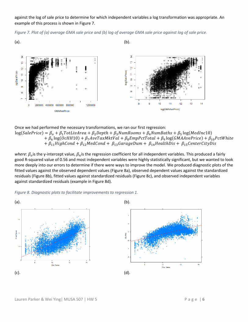
against the log of sale price to determine for which independent variables a log transformation was appropriate. An

example of this process is shown in Figure 7.

Figure 7. Plot of (a) average GMA sale price and (b) log of average GMA sale price against log of sale price.

(a).

(b).

Once we had performed the necessary transformations, we ran our first regression: log � � = � + � � � + � ℎ + � + � � ℎ + � log+ � log + � � � + � � + � log � + � ℎ�+ � ��ℎ + � + � � �� + � � ℎ � + � � �

where: � is the y-intercept value, � is the regression coefficient for all independent variables. This produced a fairly

good R-squared value of 0.56 and most independent variables were highly statistically significant, but we wanted to look

more deeply into our errors to determine if there were ways to improve the model. We produced diagnostic plots of the

fitted values against the observed dependent values (Figure 8a), observed dependent values against the standardized

residuals (Figure 8b), fitted values against standardized residuals (Figure 8c), and observed independent variables

against standardized residuals (example in Figure 8d).

Figure 8. Diagnostic plots to facilitate improvements to regression 1.

(a).

(b).

(c). (d).

Lauren Parker & Wei Ying| MUSA 507 | HW 5 P a g e | 7

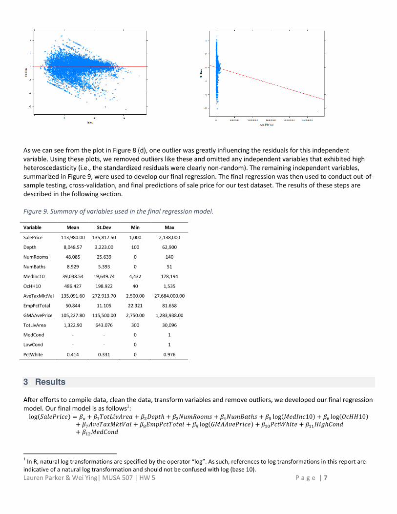
As we can see from the plot in Figure 8 (d), one outlier was greatly influencing the residuals for this independent

variable. Using these plots, we removed outliers like these and omitted any independent variables that exhibited high

heteroscedasticity (i.e., the standardized residuals were clearly non-random). The remaining independent variables,

summarized in Figure 9, were used to develop our final regression. The final regression was then used to conduct out-of-

sample testing, cross-validation, and final predictions of sale price for our test dataset. The results of these steps are

described in the following section.

Figure 9. Summary of variables used in the final regression model.

Variable Mean St.Dev Min Max

SalePrice 113,980.00 135,817.50 1,000 2,138,000

Depth 8,048.57 3,223.00 100 62,900

NumRooms 48.085 25.639 0 140

NumBaths 8.929 5.393 0 51

MedInc10 39,038.54 19,649.74 4,432 178,194

OcHH10 486.427 198.922 40 1,535

AveTaxMktVal 135,091.60 272,913.70 2,500.00 27,684,000.00

EmpPctTotal 50.844 11.105 22.321 81.658

GMAAvePrice 105,227.80 115,500.00 2,750.00 1,283,938.00

TotLivArea 1,322.90 643.076 300 30,096

MedCond - - 0 1

LowCond - - 0 1

PctWhite 0.414 0.331 0 0.976

3 Results

After efforts to compile data, clean the data, transform variables and remove outliers, we developed our final regression

model. Our final model is as follows1: log � � = � + � � � + � ℎ + � + � � ℎ + � log + � log+ � � � + � � + � log � + � ℎ� + � ��ℎ+ �

1 I ‘, atu al log t a sfo atio s a e spe ified the ope ato log . As su h, efe e es to log t a sfo atio s i this eport are

indicative of a natural log transformation and should not be confused with log (base 10).

Lauren Parker & Wei Ying| MUSA 507 | HW 5 P a g e | 8

where: � is the y-intercept value, � is the regression coefficient for all independent variables. All independent variables

are defined in detail in the Introduction of this report. The results of this regression are illustrated in Figure 10.

Figure 10. Linear regression: change in sale price of selected homes in Philadelphia.

Variable Estimate Std. Error t Value Pr(>|t|)

(Intercept) 1.83E+00 2.76E-01 6.634 3.40e-11 ***

TotLivArea 1.31E-04 1.69E-05 7.726 1.20e-14 ***

Depth 1.74E-05 2.78E-06 6.276 3.59e-10 ***

NumRooms -2.00E-03 4.57E-04 -4.388 1.15e-05 ***

NumBaths 9.20E-03 2.14E-03 4.304 1.69e-05 ***

log(MedInc10) 9.27E-02 2.20E-02 4.213 2.54e-05 ***

log(OcHH10) 6.51E-02 2.27E-02 2.863 0.0042 **

AveTaxMktVal 1.18E-06 1.42E-07 8.296 < 2e-16 ***

EmpPctTotal 1.08E-02 1.18E-03 9.164 < 2e-16 ***

log(GMAAvePrice) 6.30E-01 1.62E-02 38.996 < 2e-16 ***

PctWhite 3.95E-01 3.30E-02 11.984 < 2e-16 ***

HighCond -7.18E-01 4.47E-02 -16.089 < 2e-16 ***

MedCond -3.81E-01 3.82E-02 -9.964 < 2e-16 ***

Signif. codes: *** . ** . * . 5 . .

Residual standard error: 0.8664 on 12138 degrees of freedom

Multiple R-squared: 0.5599, Adjusted R-squared: 0.5595

F-statistic: 1287 on 12 and 12139 on DF, p-value: <2.2e-16

The results indicate that the independent variables explain about 56% of the observed variability in sales price (R2=0.56).

While this R-s ua ed alue is ot ega ded as high i the field of most physical sciences, it should be noted that all of

the included independent variables are highly statistically significant ( ≤ 0.001). Our results generally show logical

relationships between our independent variables and the dependent variable. For example, it is intuitive that sale price

would increase with total livable area, and our model suggests that with every additional square foot of livable area, the

sale price increases by $13,100. Similarly, our model suggests that with every additional installation of a bathroom, the

sale price increases by $9,200. This seems to be reasonable, as it likely costs on the order of $10,000 to add a bathroom

to a house. The results for the model on the training dataset can be further summarized as:

Adjusted R-squared: 0.5595

Root mean square error (RMSE): 0.8659

Mean absolute error: 0.6135

Mean absolute percent error (MAPE): 112.2%

These results suggest that, on average, our predicted values are about 112% different than our observed values. To

more deeply understand the accuracy of our model, we developed several diagnostic plots (Figure 11).

Figure 11. Plots of (a) observed versus predicted sales price, (b) observed sales price versus standardized residuals, (c)

fitted dependent values versus standardized residuals.

(a).

(b).

(c).

Lauren Parker & Wei Ying| MUSA 507 | HW 5 P a g e | 9

These plots suggest that our model predicts sales values only fairly well; two main issues are revealed by these plots: 1)

there is not a perfect fit between observed and predicted values, and 2) residuals exhibit a non-random pattern. There is

strong variability in the plot of observed and predicted values. But at the same time, the line of fit between the observed

and predicted values is not far off from the optimal 45 degree line, suggesting that our fitted values do not deviate by an

extreme amount from observed values. There is a pattern in the plot of observed sales values and standardized

residuals, indicating that we may not meet assumptions of homoscedasticity (i.e., the residuals are not completely

random), which is an issue that should be addressed. Finally, we do not see constant variation in the plot of fitted values

against standardized residuals; furthermore, there seems to be a bifurcated trend. This suggests again, that the residuals

may not be completely random, but also there may be another independent variable that we did not include that has

some explanatory power. We looked more closely at the spatial distribution of our residuals to determine if there was

some spatial auto-correlation (i.e., clustering) by mapping the residuals (Figure 12).

Figure 12. Map of (a) linear regression residuals and (b) results of Moran s I test.

(a).

(b).

Based on a visual inspection of the map of our residuals, we see that there may be some spatial auto-correlation in the

form of clustering. For example, there is a cluster of high, positive residuals in South Philly, and perhaps the smallest

error (residuals closest to zero, in pale yellow) are in Northeast Philly. We a a test fo Mo a s I in ArcGIS, which

reinforced that our residuals were spatially auto-correlated. Due to the short timeframe of this project, we could not

properly address the errors present in our model, but we recognize that including additional explanatory variables and

controlling for the non-random nature of our residuals would be important follow-up work. Perhaps a spatial regression

would be more appropriate.

We can further explore the localized error in our model by mapping mean average percent error (MAPE) by

neighborhood. Figure 13 illustrates our aggregate MAPE by neighborhood. While most of the neighborhoods with low

Lauren Parker & Wei Ying| MUSA 507 | HW 5 P a g e | 10

MAPE are those areas that contain the most open-space (e.g., the neighborhood encompassing the Wissahickon), there

are some highly populated areas where model predicted with high accuracy. Those neighborhoods include Center City

East, Chinatown, Callowhill and East Poplar.

Figure 13. Mean absolute percent error (MAPE) by neighborhood.

Cross-Validation

We then performed a 10-fold cross validation on our training dataset, where each observation was predicted by

regressing 9 other observations. In this cross-validation, we see a dramatic improvement in our predictive ability (R-

squared = 0.8224). We theorize that this improvement is biased, in part, by using a very small sample (n=10).

Variables Estimate Std. Error t value Pr(>|t|)

(Intercept) 6.53E+00 1.79E-01 36.55 < 2e-16 ***

Ken_ID 2.91E-04 2.17E-06 134.066 < 2e-16 ***

TotLivArea 3.43E-05 1.08E-05 3.186 0.00144 **

Depth -2.53E-05 1.79E-06 -14.101 < 2e-16 ***

NumRooms 5.79E-04 2.91E-04 1.99 0.04657 *

NumBaths 4.19E-03 1.36E-03 3.085 0.00204 **

logMedInc 5.79E-02 1.40E-02 4.146 3.41e-05 ***

logOcHH -1.29E-02 1.44E-02 -0.893 0.37195

AveTaxVal 1.06E-06 9.02E-08 11.739 < 2e-16 ***

EmpPct 3.68E-03 7.50E-04 4.91 9.24e-07 ***

logGMAPrice 1.92E-01 1.08E-02 17.885 < 2e-16 ***

PctWhite -3.56E-01 2.17E-02 -16.422 < 2e-16 ***

HighCond -1.92E-01 2.86E-02 -6.693 2.28e-11 ***

MedCond -6.10E-02 2.44E-02 -2.503 0.01232 *

“ig if. odes: *** . ** . * . . .

Residual standard error: 0.5501 on 12138 degrees of freedom

Multiple R-squared: 0.8226 Adjusted R-squared: 0.8224

F-statistic: 4330 on 13 and 12138 on DF, p-value: <2.2e-16

Lauren Parker & Wei Ying| MUSA 507 | HW 5 P a g e | 11

We see in the plots of Figure 14 that similar errors arise, in that there is a non-random distribution of residuals against

observed and predicted values (i.e., heteroscedasticity), and that there is non-constant variation.

Figure 14. Results of 10-fold cross validation of training dataset, with (a) observed sales prices against residuals, and (b)

predicted values against residuals.

(a).

(b).

Out-of-Sample Training Prediction

Next, we performed an out-of-sample prediction by randomly dividing our dataset into two subsets: 1) a sub-training

dataset composed of 75% of the observations, and 2) a sub-testing dataset consisting of 25% of the observations. We

regressed the sub-training dataset onto the sub-testing dataset using the same independent variables as noted in the

model above, and got the following results:

Adjusted R-squared: 0.5624

Root mean square error (RMSE): 0.8533

Mean absolute error: 0.6174

Mean absolute percent error (MAPE): 106.2%

These results suggest again, that while the model does have some strong explanatory power, there is still some error

that has not been properly accounted for.

Prediction for Testing Dataset

We then used our original regression to predict alues fo hi h e ha e o sales p i es i.e., the test dataset . We

can see in Figure 15 how the spatial distribution of home prices is translated from the training dataset to the predicted

dataset. Generally, in both maps, more expensive houses are clustered in Center and Old City, and there are pockets of

lower priced houses in Mantua, southern West Philly and areas around Olney. We interpret that these similarities

between the actual and predicted data are suggestive of a fairly accurate model.

Lauren Parker & Wei Ying| MUSA 507 | HW 5 P a g e | 12

Figure 15. Map of predicted values in (a) the training dataset (n=12,152), (b) the test dataset (n=2,154).

(a).

(b).

4 Discussion

Depending on the application, R-squared values of 0.56 could either be considered a breakthrough or something to be

immediately discounted. As it relates to predicting home prices in Philadelphia, our model would perhaps fall between

those two extremes. We recognize that our model has some residual error, only moderate explanatory power, positive

spatial auto-correlation, and possibly some multi-collinearity between independent variables. However, when

comparing the overall spatial distribution of prices in our actual versus predicted dataset, we see similar trends emerge

suggesting that our model can produce some quality predictions. Also, there are areas across Philadelphia for which our

residual error was very low; more specifically, if we look at the mean absolute percent error (MAPE) by neighborhood

we see that there are several key neighborhoods close to Center City for which our error is very low.

In our analysis, we found that three of our independent variables strongly improved the model: employment rate,

median household income and the average price of homes within each geographic market area (GMA). We can imagine

why this may be true: it seems reasonable to think that those areas with a higher employment rate have residents who

can afford a more expensive house, and likewise, those households who earn a higher income may be able to willing to

spend more on a house. We believe that, despite our spatially-dependent errors, we have accounted for some spatial

variability in price by using the average price of homes within each GMA. The GMAs are already spatial in nature, in that

they spatially divide the city into groups of common housing markets, so it is not such a reach to expect that this variable

controlled for some of our spatial auto-correlation.

5 Conclusion

Given the short timeframe, we believe our model is a great start. We were successful in trying out 44 different variables

and determined which of these variables would best improve the explanatory power of the model. In the end, our

Lauren Parker & Wei Ying| MUSA 507 | HW 5 P a g e | 13

model can explain about 56% of the variability in home prices in Philadelphia. We identified issues in our model, such as

spatial auto-correlation and non-random patterns in our residuals, and recognize that these are areas where we could

improve our model given more time. At this point, however, we do not recommend this model to Zillow. According to

the Zillow website, their current forecasting model has a median error of 6%, with 86.2% of homes forecasting within

20% of the sale price. Our current model does not predict within those narrow margins of error and it would require

additio al a al ses to i p o e ou odel to eet )illo s ta get fo e asti g a ilities.

In addition to spending more time to control for our residuals by perhaps performing a spatial regression, we could

i o po ate additio al datasets that a e used i )illo s fo e asti g odel. P o ided we could procure the datasets, we

could try to include: historical sale values, property tax rate, construction costs, and percentage of loans that are

subprime, as these a e additio al datasets that a e i luded i )illo s fo e asti g odel. In our current analysis, we

were not able to include these variables because they were either not publicly available at no-cost, or the geographic

level at which we could obtain the data were too aggregate (e.g., county).