Housing Wealth and Consumption: Did the Linkage Increase in the 2000s?

Mark DomsFederal Reserve Bank of San Francisco

Wendy DunnBoard of Governors

Daniel VineBoard of Governors

Household Indebtedness, House Prices and the Economy, September 19-20, 2008

Sveriges Riksbank

Thanks to,

• Tack till Riksbanken

• Martin who received a draft so late

• Great research assistants

Usual caveat

The results presented here do not necessarily reflect the views of the Federal Reserve Bank of San Francisco or the Board of Governors of the Federal Reserve System.

Summary1. There are several reasons to suspect that the linkage

between housing wealth and consumption may have increased in the 2000s relative to previous decades.

2. Using 3 different datasets, 2 of which are new, and using equations similar to those used to forecast consumption, we find support for this idea.

3. The results appear to be largely driven by populations that are traditionally considered credit constrained.

4. These results could have potentially important implications for the outlook of the U.S. economy.

Outline1. Motivation

2. Possible reasons why the linkage between housing wealth and consumption may have increased

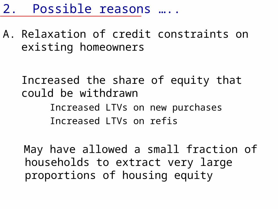
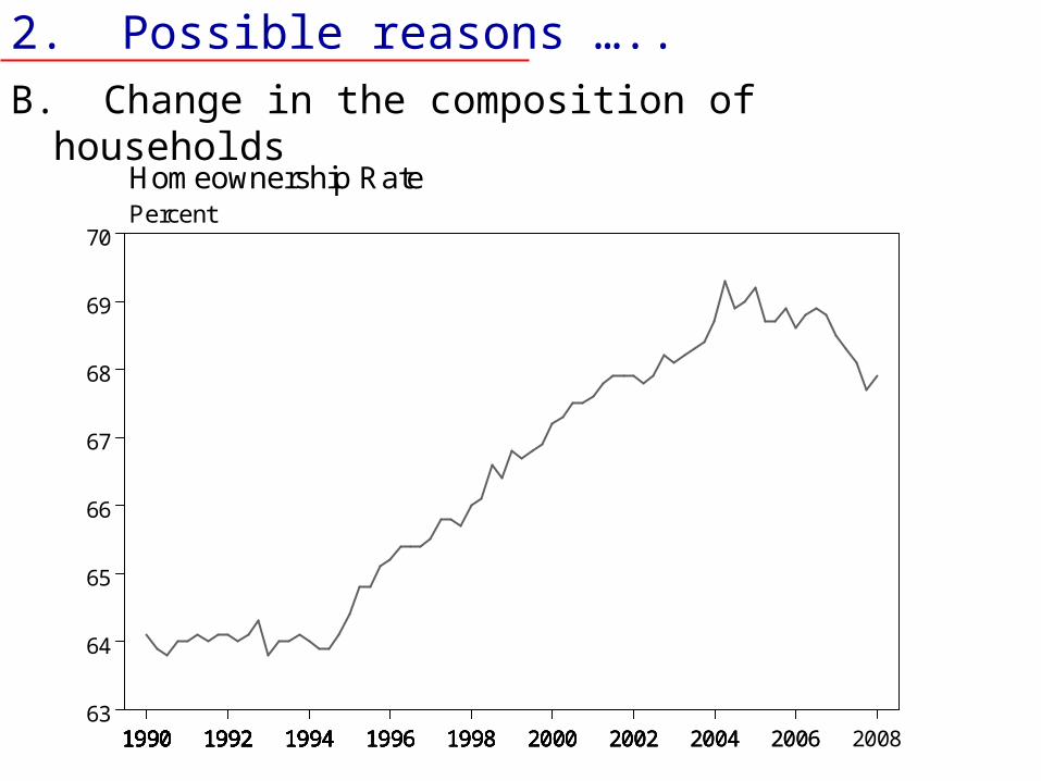
• Relaxation of credit constraints•On existing homeowners•Change in the composition of homeowners

• Changes in attitudes/behaviors

Outline, cont’d

3. Data• Two regional-level panel datasets• One individual-level dataset

4. Estimates• Estimate a large variety of models • Test whether the linkage between consumption

and house prices increased in the 2000s• To the extent possible, which areas/people had

the largest changes.

Outline, cont’d

5. Implications

6. Future work

1. Motivation

Real housing wealth

Real housing equity

Real housing debt

2

6

10

14

18

22

2

6

10

14

18

22

19901990 19941990 1994 19981990 1994 1998 20021990 1994 1998 2002 2006Source: Board of Governors

Levels, 2008 trillions, log scale

Figure 1: Real Housing Wealth, Equity, and Debt1990Q1-2008Q2

1. Motivation

Real housing equity

Real housing debt

3

5

7

9

11

3

5

7

9

11

19901990 19941990 1994 19981990 1994 1998 20021990 1994 1998 2002 2006Source: Board of Governors

Levels, 2008 trillions, log scale

Figure 1: Real Housing Equity and Real Housing Debt1990Q1-2008Q2

1. Motivation

Equity share ofhousing wealth

Real house prices

47

50

53

56

59

62

Perc

ent

-8

-6

-4

-2

0

2

4

6

8

Perc

ent c

hang

e

19921992 19941992 1994 19961992 1994 1996 19981992 1994 1996 1998 20001992 1994 1996 1998 2000 20021992 1994 1996 1998 2000 2002 20041992 1994 1996 1998 2000 2002 2004 20061992 1994 1996 1998 2000 2002 2004 2006 2008Source: Board of Governors and OFHEO.

Figure 2: Equity Share of Housing Wealth andYear-Over-Year Change in Real House Prices,1990Q1-2008Q2

1. Motivation

-50

0

50

100

150

200

1992 1994 1996 1998 2000 2002 2004 2006 2008Source: Board of Governors.

Billions of 2008 dollarsNet Issuance of Home Equity Loans

One way to extract equity

2. Possible reasons why the linkage between housing wealth and consumption may have increasedA. Relaxation of credit constraints on existing

homeowners– Reduction in costs of extracting equity • As a result of large investments made in IT, the cost of

extracting equity from homes has fallen significantly since the 1990s – home equity lines of credit, refis, reverse mortgages

2. Possible reasons …..

A. Relaxation of credit constraints on existing homeowners

Increased the share of equity that could be withdrawn

Increased LTVs on new purchases

Increased LTVs on refis

May have allowed a small fraction of households to extract very large proportions of housing equity

63

64

65

66

67

68

69

70

19901990 19921990 1992 19941990 1992 1994 19961990 1992 1994 1996 19981990 1992 1994 1996 1998 20001990 1992 1994 1996 1998 2000 20021990 1992 1994 1996 1998 2000 2002 20041990 1992 1994 1996 1998 2000 2002 2004 20061990 1992 1994 1996 1998 2000 2002 2004 2006 2008

PercentHomeownership Rate

2. Possible reasons …..

B. Change in the composition of households

2. Possible reasons …..

C. Behavioral changes

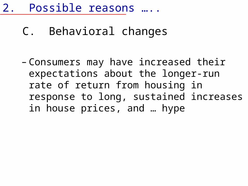
– Consumers may have increased their expectations about the longer-run rate of return from housing in response to long, sustained increases in house prices, and … hype

Figure 5: Example of Changes in Future House Price Appreciation

2. Possible reasons …..

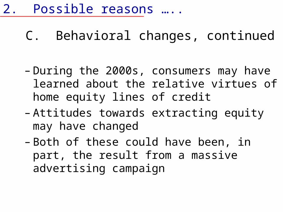
C. Behavioral changes, continued

– During the 2000s, consumers may have learned about the relative virtues of home equity lines of credit

– Attitudes towards extracting equity may have changed

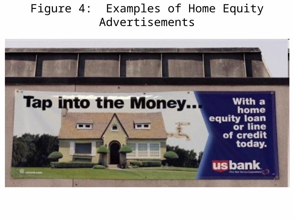
– Both of these could have been, in part, the result from a massive advertising campaign

Figure 4: Examples of Home Equity Advertisements

Figure 4: Examples of Home Equity Advertisements

3. DataMicro datasets with good measures of consumption are difficult to come by for the U.S.

We develop 2 regional panel datasets with measure of consumption and the measures of other variables typically used in consumption models

1 individual-level dataset

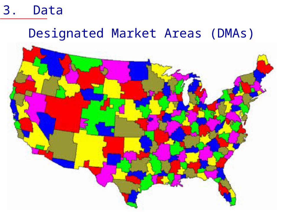
3. DataRegional datasets

1. New motor vehicle retail sales in over 180 U.S. markets (DMAs) from 1989q1 to 2007Q3

2. Quarterly taxable sales in 28 California metropolitan statistical areas (MSAs) from 1990Q1 to 2007Q1.

We merge measures of personal income, unemployment rate, housing wealth, house prices, financial wealth, transfer income …. into both datasets

3. Data

3. Data

The second covers quarterly taxable sales in 28 California metropolitan statistical areas (MSAs) from 1990Q1 to 2007Q1

• Construct other variables in the same way as for the motor vehicle/DMA dataset

• Not as many observations as the DMA dataset, but covers a larger portion of consumption

3. DataTime-Series Variance Across DMAs for Key Variables

-5

0

5

10

15

1990 1995 2000 2005 2010

Log Change in Real House Prices

-4

-2

0

2

4

6

1990 1995 2000 2005 2010

Log Change in Employment

-2

0

2

4

6

8

1990 1995 2000 2005 2010

Log Change in Real Income

-20

-10

0

10

20

1990 1995 2000 2005 2010

Log Change in Motor Vehicle Sales

3. DataTime-Series Variance Across CA MSAs for Key Variables

-10

0

10

20

30

1990 1995 2000 2005

Log Change in Real House Prices

-5

0

5

10

15

1990 1995 2000 2005

Log Change in Employment

-5

0

5

10

15

1990 1995 2000 2005

Log Change in Real Income

-10

-5

0

5

10

1990 1995 2000 2005

Log Change in Real Sales

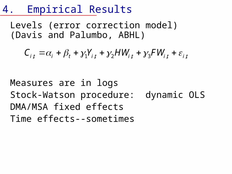
4. Empirical Results

Identification

• Although there may be a bias, we do not believe that the bias would necessarily increase over time.

• Second, we do not believe that it would increase more for some segments of the population than others

4. Empirical Results

Estimate a wide variety of models, we’ll show two main classes with our datasets

– Growth rates on growth rates versus levels (error-correction)

– Split our sample by time, credit scores, … to see, to some extent, how our results align with others

– How are variables measured

4. Empirical Results

Growth rates on growth rates (a la Case, Quigley, and Shiller; Gan; Campbell and Cocco)

, , ,

, 1 ,

,

,

,

,

,

log( ) log( ) log( )

log( ) log( )

is a measure of consumption (several measures)

is housing wealth (variety of measures)

is personal income

is financial w

i t H i t Y i t

C i t F i t

i i t t i t

i t

i t

i t

i t

C H Y

C F

L T

C

H

Y

F ealth (variety of measures)

4. Empirical ResultsOn a quarterly basis, most of variance in the log change in housing wealth arrives from changes in house prices.

We examine unadjusted and adjusted changes in house prices

, , 1 ,

1 , 4 , 4

, 1 ,

log( ) log( ) log( )

log( )

i t i i t t H i t Y i t

U i t U i t

i i t t P i t i t

HPI D T HPI Y

unemployment unemployment

L T P

4. Empirical Results

Did increaseover time?

Weestimate by decadeand test

if increased.

H

H

H

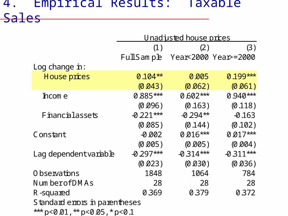
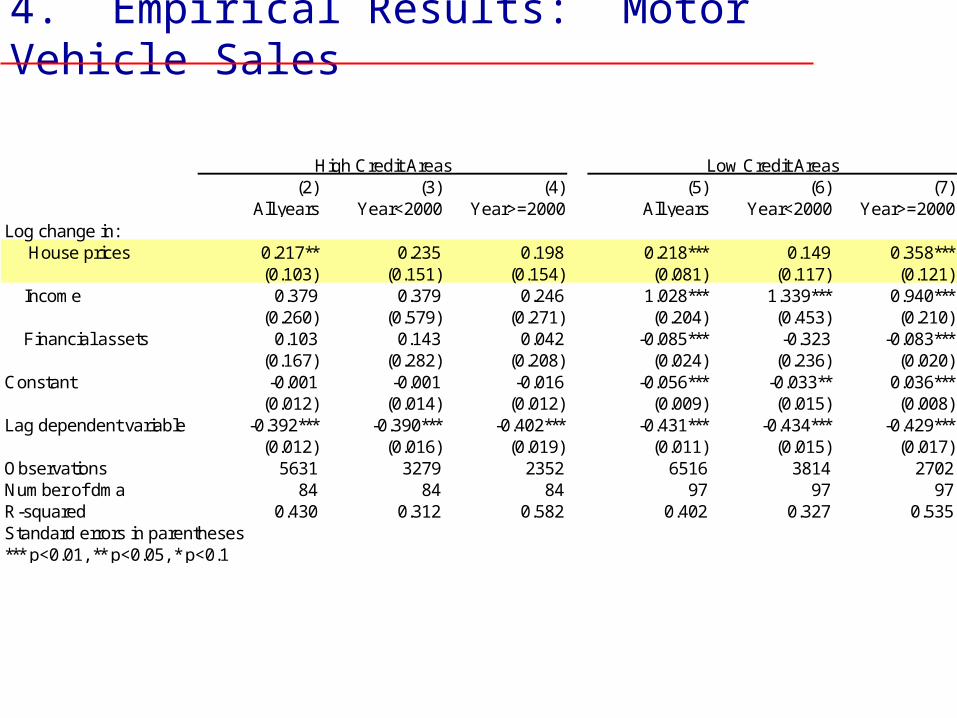
4. Empirical Results: Taxable Sales

(1) (2) (3)Full Sample Year<2000 Year>=2000

Log change in: House prices 0.104** 0.005 0.199***

(0.043) (0.062) (0.061) Income 0.885*** 0.602*** 0.940***

(0.096) (0.163) (0.118) Financial assets -0.221*** -0.294** -0.163

(0.085) (0.144) (0.102)Constant -0.002 0.016*** 0.017***

(0.005) (0.005) (0.004)Lag dependent variable -0.297*** -0.314*** -0.311***

(0.023) (0.030) (0.036)Observations 1848 1064 784Number of DMAs 28 28 28R-squared 0.369 0.379 0.372Standard errors in parentheses*** p<0.01, ** p<0.05, * p<0.1

Unadjusted house prices

4. Empirical Results: Taxable Sales

(7) (8) (9)Full Sample Year<2000 Year>=2000

Log change in: House prices 0.077 -0.055 0.249***

(0.052) (0.072) (0.077) Income 0.951*** 0.660*** 0.931***

(0.096) (0.169) (0.118) Financial assets -0.226** -0.291* -0.179*

(0.089) (0.162) (0.103)Constant -0.002 0.062*** 0.006

(0.005) (0.016) (0.005)Lag dependent variable -0.305*** -0.339*** -0.308***

(0.024) (0.031) (0.039)Observations 1652 952 700Number of DMAs 28 28 28R-squared 0.354 0.361 0.374Standard errors in parentheses*** p<0.01, ** p<0.05, * p<0.1

House prices adjusted by current, past, and future economic conditions

4. Empirical Results: Motor Vehicle Sales

(1) (2) (3)Full Sample Year<2000 Year>=2000

Log change in: House prices 0.159*** 0.052 0.336***

(0.054) (0.078) (0.081) Income 0.720*** 1.081*** 0.575***

(0.153) (0.348) (0.157) Financial assets -0.075*** -0.228 -0.074***

(0.024) (0.171) (0.021)Constant -0.051*** 0.013 0.037***

(0.007) (0.009) (0.006)Lag dependent variable -0.419*** -0.422*** -0.418***

(0.008) (0.010) (0.012)Observations 13450 7698 5752Number of DMAs 186 186 186R-squared 0.392 0.298 0.537

Unadjusted house prices

4. Empirical Results: Motor Vehicle Sales

(7) (8) (9)Full Sample Year<2000 Year>=2000

Log change in: House prices 0.195*** 0.140 0.280***

(0.064) (0.093) (0.097) Income 0.776*** 1.013*** 0.611***

(0.159) (0.360) (0.166) Financial assets -0.077*** -0.141 -0.076***

(0.025) (0.182) (0.021)Constant -0.030*** 0.001 0.041***

(0.007) (0.009) (0.007)Lag dependent variable -0.424*** -0.428*** -0.420***

(0.008) (0.011) (0.013)Observations 12147 7093 5054Number of DMAs 181 181 181R-squared 0.399 0.300 0.548Standard errors in parentheses*** p<0.01, ** p<0.05, * p<0.1

House prices adjusted by current, past, and future economic conditions

4. Empirical Results

For what groups?

Split the sample in many ways• Income• Rapid/not rapid house price increases• ….

Measures that might be related to credit constraints• Denial rates• Average credit scores

4. Empirical Results: Taxable Sales

(2) (3) (4) (5) (6) (7)

All years Year<2000 Year>=2000 All years Year<2000 Year>=2000Log change in: House prices 0.049 -0.075 0.093 0.064 -0.050 0.304***

(0.099) (0.155) (0.125) (0.067) (0.086) (0.114) Income 1.244*** 0.598* 1.310*** 0.513*** 0.510** 0.608**

(0.160) (0.360) (0.182) (0.157) (0.206) (0.259) Financial assets -0.282** -0.237 -0.261* -0.163 -0.410 -0.015

(0.120) (0.229) (0.134) (0.141) (0.250) (0.177)Constant 0.001 0.021*** -0.016*** 0.013** 0.023*** -0.000

(0.007) (0.007) (0.006) (0.007) (0.006) (0.007)Lag dependent variable -0.370*** -0.381*** -0.385*** -0.269*** -0.287*** -0.259***

(0.034) (0.044) (0.055) (0.036) (0.047) (0.057)Observations 826 476 350 826 476 350Number of dma 14 14 14 14 14 14R-squared 0.432 0.413 0.468 0.344 0.360 0.326Standard errors in parentheses*** p<0.01, ** p<0.05, * p<0.1

High Credit Areas Low Credit Areas

4. Empirical Results: Motor Vehicle Sales

(2) (3) (4) (5) (6) (7)All years Year<2000 Year>=2000 All years Year<2000 Year>=2000

Log change in: House prices 0.217** 0.235 0.198 0.218*** 0.149 0.358***

(0.103) (0.151) (0.154) (0.081) (0.117) (0.121) Income 0.379 0.379 0.246 1.028*** 1.339*** 0.940***

(0.260) (0.579) (0.271) (0.204) (0.453) (0.210) Financial assets 0.103 0.143 0.042 -0.085*** -0.323 -0.083***

(0.167) (0.282) (0.208) (0.024) (0.236) (0.020)Constant -0.001 -0.001 -0.016 -0.056*** -0.033** 0.036***

(0.012) (0.014) (0.012) (0.009) (0.015) (0.008)Lag dependent variable -0.392*** -0.390*** -0.402*** -0.431*** -0.434*** -0.429***

(0.012) (0.016) (0.019) (0.011) (0.015) (0.017)Observations 5631 3279 2352 6516 3814 2702Number of dma 84 84 84 97 97 97R-squared 0.430 0.312 0.582 0.402 0.327 0.535Standard errors in parentheses*** p<0.01, ** p<0.05, * p<0.1

High Credit Areas Low Credit Areas

4. Empirical Results

Levels (error correction model) (Davis and Palumbo, ABHL)

Measures are in logsStock-Watson procedure: dynamic OLS DMA/MSA fixed effectsTime effects--sometimes

, 1 , 2 , 3 , ,i t i t i t i t i t i tC Y HW FW

4. Empirical Results: Levels, Motor Vehicles

(1) (2) (3) (4) (5)Log house, 1 0.156*** 0.148*** 0.0413***

(0.00975) (0.00972) (0.0143)Log house, 2 0.100***

(0.0108)Log house, 3 0.0898***

(0.00699)Log house,1 post 1999 0.0893***

(0.0148)Log financial assets 0.0781*** 0.129*** 0.0844*** 0.0546***

(0.0128) (0.0128) (0.0132) (0.0157)Log income 1.136*** 1.036*** 1.011*** 1.132*** 1.051***

(0.0168) (0.0253) (0.0237) (0.0233) (0.0332)Constant -6.400*** -8.142*** -5.573*** -4.176*** -6.136***

(0.120) (0.333) (0.375) (0.310) (0.535)Observations 13419 13393 13393 13239 13393Number of dma 186 186 186 184 186R-squared . . . . .Standard errors in parentheses*** p<0.01, ** p<0.05, * p<0.1

4. Empirical Results

(1) (2)Log of sales gap (actual-predicted) -0.252*** -0.155***

(0.009) (0.008)Lagged log of housing wealth 0.172***

(0.033)Lagged log of financial wealth 0.086

(0.082)Constant 0.012*** 0.047***

(0.001) (0.007)Observations 12707 12707Number of dma 186 186R-squared 0.338 0.570Standard errors in parentheses*** p<0.01, ** p<0.05, * p<0.1

Adjustment Dynamics: Log Change in Motor Vehicle Sales

4. Empirical Results: SIPPSurvey of Income and Program Participation (SIPP)– complicated survey structure

Did a family buy a new car over the past year?

Examine only those families that did not move in consecutive years.

Control for existing car stock, income, age, …… and log change in house value.

Results not as robust as in the other datasets.

4. Empirical Results: SIPP

(1) (2) (3)

Full sample Year<2000 Year>2000Log change in house value 0.009 -0.002 0.014

(0.006) (0.009) (0.007)*Age 0.000 -0.000 0.000

(0.000) (0.000) (0.000)Education -0.001 0.001 -0.002

(0.001) (0.001) (0.001)**Log change in income 0.014 0.036 0.002

(0.004)** (0.010)** (0.005)

4. Empirical Results: SIPP

Age<45Age<45,

Year<2000Age<45,

Year>2000Log change in house value 0.038 0.012 0.050

(0.012)** (0.020) (0.012)**Age -0.001 -0.002 -0.001

(0.000)* (0.001) (0.001)Education 0.001 0.002 -0.000

(0.001) (0.002) (0.002)Log change in income 0.017 0.050 -0.002

(0.007)* (0.017)** (0.008)

5. Implications

• Do these results help in forecasting

• How much of a drag will the decline in house prices have on the economy

5. Implications

Assumed housing wealth effect 15.0 20.0 25.0Modest 1.0 0.3 0.4 0.5

25% greater 1.3 0.4 0.5 0.650% 1.5 0.5 0.6 0.8100% 2.0 0.6 0.8 1.0

FRB/US 3.5 1.1 1.4 1.825% greater 4.4 1.3 1.8 2.250% 5.3 1.6 2.1 2.7100% 7.0 2.1 2.9 3.6

The assumed housing wealth effect is in percent.The numbers in the table are in percentage points of consumption

Table 11: Estimates of the Direct Restraints to Consumption Growth from a Decline in Housing Wealth

Assumed decline in real housing wealth (in percent)

6. Future work• Forecast errors

• Symmetry– Extending our datasets

• Identification

• PSID

• Labor supply and wealth shocks

1. Motivation

0

20

40

60

80

Pe

rcen

t

0-20 20-40 40-60 60-80 80-90 90-100

Note: X-axis ranges represent percentiles of income. Liquid financial wealth isdefined as total financial assets minus quasi-liquid retirement accounts.Source: Survey of Consumer Finances.

Percent of Households WhoseNet Housing Wealth Exceeds Net Financial Wealthby Income Percentile, 2004

Total financial wealthLiquid financial wealth

1. Motivation

0

20

40

60

80

Pe

rcen

t

0-20 20-40 40-60 60-80 80-90 90-100

Note: X-axis ranges represent percentiles of income. Liquid financial wealth isdefined as total financial assets minus quasi-liquid retirement accounts.Source: Survey of Consumer Finances.

Percent of Households WhoseNet Housing Wealth Exceeds Net Financial Wealthby Income Percentile, 1995

Total financial wealthLiquid financial wealth

3. Data

Designated Market Areas (DMAs)