78
Waste Heat Recovery HOUSSAM ACHKOUDIR NAOWAR HANNA Master of Science Thesis Stockholm, Sweden 2011

Waste Heat Recovery
HOUSSAM ACHKOUDIR
NAOWAR HANNA
Master of Science Thesis
Stockholm, Sweden 2011

Waste Heat Recovery
Study of the efficiency potential of water based Rankine WHR system
with a piston expander
Houssam Achkoudir
Naowar Hanna
Master of Science Thesis MMK 2011:21 MFM 137
KTH Industrial Engineering and Management
Combustion Engine
SE-100 44 STOCKHOLM
Examensarbete MMK 2011:21 MFM 137
Studie av verkningsgrad potentialen för ett vatten baserat
Waste Heat Recovery system med kolvexpander
Houssam Achkoudir, [email protected] Naowar Hanna, [email protected]
Godkänt 2011-02-25
Examinator Hans-Erik Ångström, KTH
Handledare Gustav Ericsson, KTH
Uppdragsgivare Scania AB
Kontaktperson Johan Linderyd, Scania
Sammanfattning
En ånganna monterades i EGR (Exhaust Gas Recirculation) slingan på en 12,7 liters Scania Euro V
motor (DC1306). En modell som beskriver Rankine cykel togs fram med vatten som köldmedium i
simuleringsverktyget GT-Power. Ångpannan i GT-power modellen kalibrerades m.h.a experimentell
data.
Simuleringarna visade att det optimala ångtrycket, det trycket där högst effekt kan erhållas från
expandern, är beroende av EGR temperaturen. Det innebär att ju högre EGR inloppstemperatur
desto högre optimalt ångtryck. EGR temperaturen i punkt 2 i ESC cykeln är 514˚ C för denna motor,
vilket resulterar i ett optimalt tryck på 120 bar enligt simuleringen. Vidare analyserades den optimala
överhettningsgraden, vilket innebär antalet grader som ångan uppvärms vid konstant tryck efter att
allt vatten har förångats. Simuleringarna visar att högst effekt i expandern erhålls då ångan
överhettas 10 grader, alltså den lägsta överhettningsandelen. Detta beror på att ångeffekten från
ångpannan är högst vid lägst andel överhettningsgrad, vilket beror på ett högre vatten flöde.
Simuleringen visar att EGR temperaturen är viktigare än EGR flödet. Ett sätt att öka EGR
temperaturen är genom att tillsatselda. Detta innebär att spruta in bränsle i avgasröret. Beräkningar
visar dock att det är lönsammare att spruta in bränslet direkt i förbränningsrummet. Att öka EGR
temperaturen med 150˚C skulle resultera i ca 2,5 kW ökning i erhållen effekt från exandern. Att
spruta in samma dieselflöde i förbränningsrummet skulle medföra en effektökning med ca 5,2 kW
från motorn.
Vid det optimala ångtrycket samt 10 graders överhettad ånga minskar bränsleförbrukningen för
punkt 2 i ESC cykeln med 1,4 %. WHR (Waste Heat Recovery) systemet verkningsgrad ligger på 18,4
%. Vid montering av ytterliggare en ångpanna efter turbinen för att på så vis utnyttja energin i
avgasflödet, istället för bara i EGR gaserna, skulle bränsleförbrukningen minska med 3,41 %.

Master of Science Thesis MMK 2011:21 MFM 137
Study of the efficiency potential for a water based
Waste Heat Recovery system with piston expander
Houssam Achkoudir, [email protected] Naowar Hanna, [email protected]
Approved 2011-02-25
Examiner Hans-Erik Ångström, KTH
Supervisor Gustav Ericsson, KTH
Commissioner Scania AB
Contact person Johan Linderyd, Scania
Abstract
An evaporator was mounted in the EGR loop of a 12,7 liter Scania Euro V engine (DC1306). A model
describing the Rankine cycle was developed with water as refrigerant in the simulation tool GT-
Power. The evaporator in the GT-Power model was calibrated with experimental data.
The simulations showed that the optimal vapor pressure where the maximum power available from
the expander is obtained depends on the EGR temperature. Higher EGR inlet temperature leads to
increased optimal vapor pressure. The EGR temperature in case 2 of the ESC cycle is 514 °C for the
engine above, this result in an optimal vapor pressure of 120 bar according to the simulation. The
optimum level of superheating was analyzed, which means the amount of degrees the vapor
temperature is raised at a constant pressure after all the water is evaporated. The simulations show
that the highest power in the expander was obtained when the steam was superheated by 10
degrees, i.e. the lowest level of superheating. The steam power after the evaporator is highest at the
lowest level of superheating, because of the higher refrigerant flow.
Simulations show that the EGR temperature has a bigger impact than the EGR flow. One way to
increase the EGR temperature is by supplementary burning, which means injecting fuel into the
exhaust pipe. Calculations show that it is more profitable to inject fuel directly into the combustion
chamber. Increasing the EGR inlet temperature with 150 °C would result in 2,5 kW higher power
output from the expander. Injecting the same fuel flow in the combustion chamber the engine power
output increases with 5,2 kW.
Operating point 2 in the ESC cycle reduces the fuel consumption with 1,4 % if run at the optimal
steam pressure of 120 bar and 10 degrees of superheated vapor. The reduction of the fuel
consumption would be 3,41 %, if the power in the exhaust mass flow would be utilized by integrating
another evaporator after the turbine.

Acknowledgements
The two supervisors Gustav Ericsson and Johan Linderyd have been very supporting and helped us
trough the project whenever we needed help, and guided us to the right solution. We want to thank
them both for all the help in this project.
We also want to thank our two lab mechanics, Jack Ivarsson and Bengt Aronsson, for helping us
mount the evaporator on the engine and solve the problems that occurred during the experiments.
We also thank Sten Dahlman who build the evaporator and Peter Platell (Ranotor) for letting us use
the evaporator and helped us to understand the Rankine cycle.

Table of contents
Nomenclature .....................................................................................................................................8
1. Introduction ....................................................................................................................................1
1.1 Background ...............................................................................................................................2
1.1.1 Rankine cycle .....................................................................................................................2
1.1.2 Superheated vapor ............................................................................................................3
1.1.3 Working fluid .....................................................................................................................5
1.1.4 Subcritical and supercritical cycle.......................................................................................5
1.1 Problem definition....................................................................................................................8
1.2 Boundaries ...............................................................................................................................8
1.4 Sources of error ........................................................................................................................8
2. Method ......................................................................................................................................... 10
2.1 GT-Power ............................................................................................................................... 10
2.1.1 Evaporator ....................................................................................................................... 10
2.1.2 Expander ......................................................................................................................... 12
2.1.3 Condenser ....................................................................................................................... 13
2.1.4 Pump & Receiver ............................................................................................................. 14
2.2 Setting up the system ............................................................................................................. 15
2.3 The engine test ....................................................................................................................... 18
2.3.1 Experimental set-up......................................................................................................... 18
2.3.2 Operation points and testing ........................................................................................... 20
2.4 Performance calculation ......................................................................................................... 22
2.4.1 Supplementary burning ................................................................................................... 23
3. Result............................................................................................................................................ 24
3.1 Experimental results ............................................................................................................... 24
3.1.1 Transient response .......................................................................................................... 29
3.2 GT-Power Results .................................................................................................................... 32
3.2.1 EGR temperature variation .............................................................................................. 33
3.2.2 EGR Flow variation ........................................................................................................... 38
3.2.3 Fuel consumption reduction ............................................................................................ 40
3.2.4 Optimizing the system ..................................................................................................... 41
3.2.5 The ESC driving cycle ....................................................................................................... 44
3.2.6 Exhaust flow .................................................................................................................... 47

3. Discussion ................................................................................................................................. 49
4. Conclusion ................................................................................................................................ 52
5. Future work .............................................................................................................................. 53
7. References .................................................................................................................................... 54
8. Appendix....................................................................................................................................... 55
8.1 Condenser Data....................................................................................................................... 55
8.2 Pump, Expander & Reciever .................................................................................................... 58
8.3 GT-Power results ..................................................................................................................... 58
8.3.1 EGR temperature variation ............................................................................................... 58
8.3.2 EGR flow variation ............................................................................................................ 60
8.3.4 Optimizing the system ...................................................................................................... 62
8.4 Evaporator calibration ......................................................................................................... 67

Nomenclature
HC - Unburned hydrocarbons
GHG - Green House Gases
WHR - Waste Heat Recovery
EGR - Exhaust gas recirculation
GT-Power – Is an industry standard engine simulation tool that is specially designed for both steady
state and transient simulation
L - Liqiud
V - Vapor
CP - Critical Point
Hp - Horse power
T-S diagram – Temperature Entropy diagram
PID regulator – Proportional Integral Derivate regulator
ESC cycle – European Stationary Cycle
VGT – Variable Geometry Turbocharger
- Heat flow rate to the system (energy per unit time)
- Heat flow rate from the system (energy per unit time)
- Mechanical power consumed by or provided to the system (energy per unit time)
- Steam power (power input to the expander)
- Heat transfer area
- Flow area
r - Radius
- Number of tubes
- The length of a micro tube, which is 3 m
- The power output from the evaporator
- The change in specific enthalpy across the evaporator
- The mass flow of the refrigerant
- Evaporator’s temperature efficiency based on the cooling ability
- The evaporator’s efficiency could also be described as how good the evaporator is in terms
of heating up the refrigerant
– The inlet cooling water temperature to the condenser
– The inlet cooling water pressure to the condenser
- The cooling water mass flow
– The cooling water temperature out from the condenser
– The cooling water pressure out from the condenser
– The water inlet temperature (after the condenser)
- The water inlet pressure (after the condenser)
- The mass flow in the refrigerant circuit
- The inlet temperature of the refrigerant (equal to )
- The water pressure after the pump
- The outlet temperature of the EGR
- The outlet pressure of the EGR
- The inlet temperature of the EGR
- The inlet EGR pressure
- The mass flow for the EGR
- The steam temperature
- The steam pressure
- The temperature after the expander (inlet temperature to the condenser)
- The pressure after the expander (inlet pressure to the condenser)
- The turbines isentropic efficiency
- The expander power output
- The heat load in the condenser
- The change in specific enthalpy across the condenser
C - The turbulent coefficient
m - The turbulent exponent

-The Nusselts number
Re - The Reynolds number
Pr - The Prandels number
h - The film coefficient
- The reference length
k - The thermal conductivity
- The heat capacity
- The dynamic viscosity
- The cooling water density
U - The velocity of the cooling water
– The pump/turbine displacement
- The volumetric efficiency for the pump/turbine
n – Revolution per seconds for the pump/turbine
– The mass flow for the pump/turbine [kg/s]
- The inlet density for the pump/turbine
RFC - Reduction of fuel consumption
- The pump power
- The power the engine requires at the current loading point
- The WHR efficiency
- The enthalpy of the refrigerant in liquid state
- The steam enthalpy, provided by moliers diagram if temperature and pressure is known
- The steam pressure
- The water pressure while the refrigerant is in liquid state
- Enthalpy for saturated water at 20 ˚C
- The specific volume of water at 20 ˚C
- The power input to the system (to the evaporator)
- The heat capacity for EGR

- The diesel mass flow
- The diesel specific energy [J/kg]
x - The degrees the EGR is to be raised
- The efficiency of a diesel engine (assumed to be 40 %)
P1- The refrigerant pressure before the evaporator
P2- The steam pressure after the evaporator
T2-1- The steam temperature after the evaporator
T2-2- The steam temperature after the evaporator (two thermocouples)
T_A-N – Sixteen thermocouples from A-N mounted on the micro tubes inside the evaporator
1
1. Introduction
The increasing oil price is putting pressure on the industry to reduce the fuel consumption, and at the same time try to achieve the rigorous emission legislations. Also an increased focus on CO₂ and GHG (Green House Gases) driven by the concern for global warming is a strong driver to increase the efforts to develop technologies that improves fuel consumption. One way to do it is to employ a hybrid system. Hybrid generally utilizes kinetic energy recovery, the energy can be used to generate electricity and charge an electric storage device. It would work if the aim is to drive in the city where there is a lot of start/stop, however the power output for a long haul truck is constant and high, so the battery in hybrid does not last for long. Another way is to take advantage of the heat energy in the exhaust gases, by either use turbo compound or Rankine cycle. This report is based on using the Rankine cycle. By using the Rankine cycle, the heat energy from the exhaust gas can be used to heat up a pressurized fluid into vapor and obtain power by expanding the vapor. The power can be used to assist the engine by adding torque to the engine output. The energy can also be used in a hybrid system, it can be used to generate electricity and charge a battery. The aspect has been interesting for many companies, because there is a lot of energy that is wasted and can be used. However there is still a lot to understand and evaluate about the WHR system for the companies that invest in it. It is important to understand the effect of the different parameters on the WHR system. This project will evaluate and discuss the possibilities with a proposed WHR Rankine system based on water as working fluid and a special design evaporator capable of handling high steam pressures. To be able to do that, a 6 cylinder 12,7 liter Scania diesel engine (DC1306) with an evaporator mounted on the EGR-root were run. The experimental data obtained from the tests have been used to calibrate a model in GT-Power [1]. In order to investigate the performance of the entire WHR system, a condenser, pump, receiver and expander has been integrated into the model.
2
1.1 Background
In a previous project about WHR system [2], a Rankine cycle with water as refrigerant was studied.
This was done by simulating an evaporator in GT-Power, then mounting a physical evaporator in the
EGR loop of the engine. The evaporator replaced the EGR cooler, and the EGR cooler was moved
downstream the evaporator because of high EGR outlet temperature after the evaporator. The
simulation and experimental results was then compared.
The purpose of this master thesis is to simulate the entire Rankine cycle, this means integrating a
pump, expander, receiver and condenser into the model from the previous project. The objective has
been to understand the influence of different parameters, understand fuel consumption potential for
a complete system and the performance of the special designed evaporator.
1.1.1 Rankine cycle
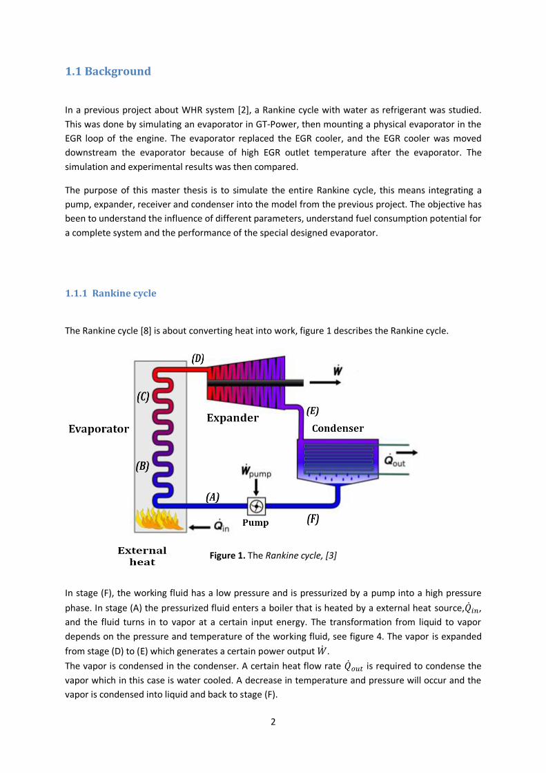
The Rankine cycle [8] is about converting heat into work, figure 1 describes the Rankine cycle.
Figure 1. The Rankine cycle, [3]
In stage (F), the working fluid has a low pressure and is pressurized by a pump into a high pressure
phase. In stage (A) the pressurized fluid enters a boiler that is heated by a external heat source, ,
and the fluid turns in to vapor at a certain input energy. The transformation from liquid to vapor
depends on the pressure and temperature of the working fluid, see figure 4. The vapor is expanded
from stage (D) to (E) which generates a certain power output .
The vapor is condensed in the condenser. A certain heat flow rate is required to condense the
vapor which in this case is water cooled. A decrease in temperature and pressure will occur and the
vapor is condensed into liquid and back to stage (F).

3
The heat source in this case is the waste heat in the EGR gases, which normally is cooled by the
coolant water. The energy losses are the power input to the pump and the energy needed to
condense the vapor. The energy needed to condense the vapor can be solved in several ways, like
using the cooling water from the engine. Mounting the evaporator in the EGR loop also means
reducing the cooling demands on the engine since theoretically there is no need for the EGR cooler.
This power can instead be used to condense the vapor.
The refrigerant circuit in GT-Power is illustrated in figure 2. The receiver in the figure is the tank
which is used to collect the water in the system.
Figure 2. WHR system
1.1.2 Superheated vapor
The different phases of the refrigerant inside the evaporator are described with a temperature-
enthalpy diagram (hT-diagram), see figure 3.
The first part of the red line, A-B, in figure 3 represents the refrigerant heating up until the boiling
point is reached. The second part, B-C, illustrates the enthalpy needed to evaporate all the
refrigerant i.e. only steam exists at point C. The final part, C-D, is the superheated part, showing the
steam superheat at constant pressure. As can be seen most of the input energy is consumed during
the second part i.e. the evaporation of the refrigerant.
Figure 3. Different states of the refrigerant

4
The letters (A-D) in figure 1 and 3 describes the same phase.
It is important that the mass flow entering the expander is fully evaporated. To achieve this, the
steam will always be at least 10 degrees superheated. It is also important to understand the
relationship between the temperature and pressure of the refrigerant, figure 4 shows the boiling
temperature for several pressures for water i.e. when the water starts to evaporate.
Figure 4. Boiling temperatures for different water pressures [4]
100
150
200
250
300
350
400
0 20 40 60 80 100 120 140 160 180 200 220 240
Tem
pe
ratu
re [˚
C]
Pressure [bar]

5
1.1.3 Working fluid
Working fluids for WHR system are according to the slope of the saturated vapor line in the
temperature-entropy diagram, usually divided into three types: dry, wet and isentropic.
Corresponding rankine cycles for the three types are shown in figure 5 [5]. L and V stands for liquid
and vapor, CP stands for critical point.
Figure 5. Three fluid types: (a) wet fluid; (b) dry fluid; (c) isentropic fluid
The wet fluid is in general inorganic fluid, such as water, ethanol, ammonia etc. As seen in the picture
above, at the end of the expansion (the red point in the picture), the wet fluid generally ends up in
the two phase area (L+V). The dry fluid however has a positive slope for the saturated vapor line, and
at the end of the expansion process the fluid ends as superheated vapor. Some examples of a dry
fluid are Benzene and R245fa. The isentropic fluid, the saturated vapor line is almost vertical in the
diagram for most temperature range, and therefore the expansion process stays as saturated vapor.
If a dry fluid is chosen as the working fluid for a Rankine cycle, a recuperator can be used after the
expander to utilize the remaining energy in the superheated vapor and improve the cycle efficiency.
The disadvantage is the enlarged cost and the packaging of the system can be difficult due to
increased number of components. The less dry the fluid is, the smaller the size of the recuperator is
required.
1.1.4 Subcritical and supercritical cycle
Depending on the temperature and pressure of a fluid, it can either be subcritical or supercritical.
Supercritical cycle is defined by pressures larger than the refrigerants critical point and subcritical by
pressures below its critical point. The refrigerants T-S diagram can show if the cycle is subcritical or
supercritical, assuming the temperature and pressure is known. Subcritical and supercritical cycles
for two different working fluids will be explained below.
Figure 6 shows a T-S diagram over a subcritical cycle for a dry fluid, R245fa, [6]. The efficiency is
at an operation parameter of: pump pressure , condensation pressure ,
evaporation temperature , condensation temperature and a maximum
superheating temperature at though R245fa becomes thermally unstable at higher
temperatures.

6
Figure 6. T-s diagram of a subcritical rankine cycle for R245fa
Supercritical cycle of the same fluid is shown in figure 7. The Rankine cycle efficiency is at an
operation parameter of: pump pressure = 100 bar, condensation pressure = 3 bar. As seen in the
picture below, the superheating is controlled such that the end of the expansion process enters two
phase state, and therefore the superheating temperature is . Subcritical cycle for this type of
fluid has a higher efficiency than supercritical cycle, though a recuperator is used in the subcritical
cycle. As seen in the figure, the expansion ratio is too large for a single-stage turbine, and therefore
some other kind of expander is needed or advanced turbine with higher expansion ratio.
Figure 7. T-s diagram of a supercritical rankine cycle for R245fa
The same cycles are shown in figure 8-9 [6] but for a wet fluid, ethanol. In the subcritical stage for
ethanol, the evaporation temperature, cycle efficiency and superheating temperature are targeted to
be the same as in R245fa.

7
Figure 8. T-s diagram of a subcritical rankine cycle for ethanol
In the supercritical stage, the operation parameters were: pump pressure = 80 bar, condensation
pressure = 1,08 bar, condensation temperature = 80 and the superheating temperature = 306 .
Under these operation parameters, the cycle efficiency was 25,5 %. Although a recuperator is used in
the subcritical cycle, the supercritical cycle have a higher efficiency. That is because the level of
superheating in subcritical cycle and supercritical cycle is closer for a wet fluid than for a dry fluid. As
described before, a dry fluid has a positive slope for the saturated vapor line, and therefore the dry
fluid’s level of superheating is limited by the end of expansion state. However, a simple turbine can
still not handle the expansion ratio.
Figure 9. T-s diagram of a supercritical rankine cycle for ethanol
In this project the working fluid will be water, which has the highest thermal stability and wetness.
The working parameter for the pump will be large, up to 180 bars. At those high pressures a 1-stage
turbine will not be sufficient.

8
1.1 Problem definition
The purpose of this master thesis is to understand the impact following parameters have on the
waste heat recovery system:
Refrigerant: Pressure and flow
EGR: Temperature and flow
The degree of superheating
A model was built where the Rankine cycle can be simulated, the model was used for conducting a
study of parameters effect. There is also a need for experimental data to validate the model,
therefore an evaporator will be mounted in the EGR loop of the engine.
The question is how much can the fuel consumption be reduced?
1.2 Boundaries
In this master thesis some boundaries have been made:
Power input to the system is only obtained from the EGR gases
Only water is used as a refrigerant
The piston expander is replaced by a turbine in GT-Power
During the experimental tests only the evaporator is mounted in the EGR loop, while in the
simulations the entire Rankine system is modeled.
In GT-Power the investigated steam pressure are between 20-180 bar while in the
experimental run the steam pressure is up to 100 bar. The evaporator is designed to tolerate
up to 250 bar.
The investigated EGR temperatures are between 290-700˚ C and the the investigated EGR
flows vary from 37-130 g/s.
During the experimental tests only the operating points in the ESC cycle were run.
1.4 Sources of error
The pressure drop is modeled just before the evaporator instead of over the evaporator in GT-Power.
This leads to a more stable model due to that the pressure drop only occurs while the refrigerant is in
the liquid state.
Assuming a constant refrigerant flow at two different pressure levels, then the pressure drop should
be higher at the lower pressure level. This depends on the higher density of the steam at the lower
pressure level. This part is not taken into consideration in the pressure drop just before the
evaporator in the GT-Power model. The pressure drop is only dependent of the mass flow. This
means that the power required by the pump should be a bit higher at low pressure levels when

9
comparing to the current results. Since the pump power is 10 times smaller than the expander
power, the affect on the final result can be neglected.
The EGR is assumed to be consisting of only air in the GT-Power model, this should have no bigger
effect since the component in GT-Power is calibrated with the data provided from the experimental
tests.
In the engine test there was a filter in the water inlet pipe, prior to the evaporator. This filter was
clogged by some black particles, even though the water was distillated and salt free. It is believed to
be an organic substance. This substance in the filter led to an increase in the pressure drop with
approximately 7-10 bar in some operation points of the ESC cycle.
The piston expander isentropic efficiency is assumed to be constant due to lack of data. Otherwise,
the isentropic efficiency of the piston expander is dependent on the filling factor. A higher level of
filling decreases the isentropic efficiency due to lower expansion rate in the piston expander.
The steam power provided from GT-Power is 1-2 % too high. This depends on the assumption
made that the heat transfer to the walls from the EGR equals the steam power, this means
neglecting some heat losses. But since the losses are of such a small magnitude the effect on the final
result should be minimal.
The EGR pressure drop during the experimental test could differ a bit since there is no pressure
transducer after the evaporator, the pressure just prior of the turbine was used.

10
2. Method
The first task was to build a model in GT-Power that represent the Rankine cycle with water as the
refrigerant. Results from experimental tests where the evaporator was mounted in the EGR loop of a
Scania euro V engine was used to calibrate the evaporator in the GT-Power model.
2.1 GT-Power
In a prior project course [2] a model was developed with the simulation tool GT-Power. The model
describes the heat transfer inside the evaporator between the refrigerant and the diesel exhaust
gases for different inlet temperatures and flows, see figure 10.
Figure 10. Basic model of the evaporator developed in project course
In this master thesis further components will be introduced in the model so the entire Rankine cycle
could be described. A pump, receiver, expander and a condenser were integrated into the old model.
2.1.1 Evaporator
The evaporator is designed and manufactured by Ranotor [7]. It possesses a special cylindrical design

11
and geometry which is made to tolerate up to 250 bar of steam pressure, see figure 11. The
refrigerant flows in micro tubes with small diameter. The purpose of the small diameter is to always
have laminar flow. The refrigerant should be equally distributed to 48 micro tubes inside the
evaporator. The exhaust gases flows around these micro tubes and heats up the water. The 48 micro
tubes are divided into two groups inside the evaporator, one group consisting of 21 micro tubes and
the other group of 28 micro tubes. This means the water has two inlets to the evaporator and the
steam exits through two outlets that comes together 20 cm after the evaporator. At each steam exit
there is a thermocouple mounted into the flow, the data from these sensors will be analyzed in order
to understand if the water is equally distributed between the two groups. There is also 16 thermo
couples mounted inside the evaporator.
Figure 11. The dimensions of Ranotors counter flow evaporator
In order to calibrate the evaporator in GT-Power the physical evaporator was mounted in the EGR
loop of a 360 hp 12.7 liter Scania engine (DC1306). Different parameters like the refrigerant flow,
EGR-flow, EGR-temperature and the refrigerant pressure were varied in several tests. The test results
were used to calibrate the evaporator in GT-Power, see appendix 8.4.
Other needed input data in GT-Power like heat transfer area and flow area were calculated
according to equations (1-2):
(1)
(2)
Where r is the radius of the micro tube, Ltube is the length of the micro tube and is the number
of the tubes.
The power output is calculated with equation 3:
(3)
represent the change in specific enthalpy across the evaporator and is the mass flow of
the refrigerant.

12
Finally the evaporator’s temperature efficiencies and was calculated with the help of
equation 4-5:
(4)
(5)
is the inlet temperature of the EGR, the outlet temperature of the EGR, the
steam temperature and finally the inlet temperature of the refrigerant.
2.1.2 Expander
The high pressure levels required in a Rankine cycle with water as the refrigerant are a problem while
using turbines, there is no single stage turbine that can handle these pressure levels. One possible
solution is to use a piston expander and a study has been made at KTH where a piston expander has
been developed for these kinds of applications [9]. The isentropic efficiency for the piston expander
depends on the volume flow rate of the vapor. This means a lower volume flow rate result in a larger
expansion rate and therefore higher isentropic efficiency for the expander. While a higher volume
flow rate leads to a decreased expansion rate which affects the isentropic efficiency negatively, see
figure 12 [10].
Figure 12. The isentropic efficiency of the expander as function of the load factor, [5]
Ideally it is best to run the expander with a low torque i.e. small filling and a high speed. This will lead
to a high isentropic efficiency. But lack of time makes it hard to build a piston expander model in GT-
13
Power. Therefore a simple turbine with a constant geometry will be used. The turbine’s speed will
represent the filling factor i.e. when the filling factor is high the speed will increase and vice versa.
Too calculate a relationship between the speed of the turbine and the isentropic efficiency is to
complex, therefore it was decided to use a constant isentropic efficiency regardless of the load
applied on the turbine in GT-Power. The isentropic efficiency was chosen to 65 %, see appendix
8.2.
If the steam leaving the expander is in the two phase area i.e. not superheated (see figure 5 and 49),
a turbine wouldn’t have worked since the turbine blades get damaged when they come in contact
with water. In case of the piston expanders this will not cause any problems. This also means a higher
power output from the expander since more energy can be utilized from the steam.
The expander power is calculated in GT-Power with equation 6:
(6)
The change in specific enthalpy across the turbine is , is the refrigerants mass flow and
is the turbines isentropic efficiency.
2.1.3 Condenser
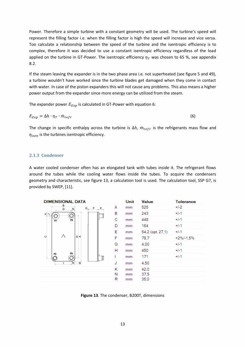
A water cooled condenser often has an elongated tank with tubes inside it. The refrigerant flows
around the tubes while the cooling water flows inside the tubes. To acquire the condensers
geometry and characteristic, see figure 13, a calculation tool is used. The calculation tool, SSP G7, is
provided by SWEP, [11].
Figure 13. The condenser, B200T, dimensions
14
The specification was 50 kW of heat load, maximum power in the EGR gases, and a working pressure
of 1,1 bar. The heat load was calculated with equation 7:
(7)
To calculate some important parameters, like the turbulent coefficient, C, and the turbulent
exponent, m, equation 8 was used:
(8)
To calculate the Nusselts number Nu and prandels number Pr, equations 9-10 was used:
(9)
(10)
Where K is the thermal conductivity, h is the film coefficient and is the heat capacity.
The reference length is another parameter required by GT-Power when building up the
condenser, equation 11 is used to calculate :
(11)
Where U is the velocity of the cooling water, Re is the Reynolds number given by the calculation tool
(SPG 7), is the density and is the dynamic viscosity.
In equation 8 the turbulent exponent m is assumed to be 0,6. According to GT-power it should be
less than 1. Therefore it is now possible to calculate the turbulent coefficient C. The flow area and
the heat transfer area are calculated in the same way as for the evaporator, see equation 1-2. For full
data see appendix 8.1.
The cooling water mass flow is kept constant at 1,697 kg/s, this value was provided by the calculation
tool, [ref ssp] meaning the condenser maximum heat load is 50 kW. The water inlet temperature to
the condenser is also kept constant at 91,5˚C regardless of loading case. This means the cooling
water outlet temperature will vary for different operating points since the cooling power needed
differs for different points.
2.1.4 Pump & Receiver
The pump used in GT-Power is a simple positive displacement pump, it is speed controlled with a PID
regulator, see appendix 8.2. Power required by the pump for different operating points is provided
by GT-Power.
The volume of the receiver is 10 liter containing only water, see appendix 8.2.

15
2.2 Setting up the system
To determine the pump and the turbine displacement equation 12 was used
(12)
Where is the volumetric efficiency, n the expanders/pumps revolutions per second, the mass
flow in kg/s and ρ the inlet density. To determine the inlet density before the turbine and the pump a
very short simulation is run. This short simulation makes it possible to see what the density is prior to
the pump and the turbine. The mass flow is decided to 10 g/s based on experimental tests
performed during the project course. The rotational speed is set so that the turbine has a speed
much higher than the pump. That depends on the geometry between the turbine and the pump,
theirs rotational speed cannot be the same.
In order to obtain a stable system three critical things must be accomplished:
The initial composition in the different components must be right
The pump must be regulated regarding speed
The turbine must be regulated regarding speed
If the system initially contains only water then there is no room for expansion i.e. when the water
boils into vapor. This will lead to uncontrollable increase in pressure in the system. Therefore initially
the correct composition in the pipes is only water before the evaporator and mostly vapor after the
evaporator. In the receiver there is only water while it is equal amount of water and vapor in the
condenser and the evaporator.
To be able to control the steam pressure in the system a PID regulator is calibrated and integrated in
the model. The input to the regulator is the total pressure measured just before the evaporator and
the output is the turbine rotational speed, see figure 14.

16
Figure 14. The marked part represents the steam pressure PID regulator in the model
If the steam pressure in the system is lower than the target then the turbines rotational speed will be
decreased in order to raise the pressure and vice versa.
As mentioned earlier it is also desirable to control the refrigerant flow in the system. This is done by
integrating another PID regulator where the input is the temperature after the evaporator. The
output of this regulator is the pumps rotational speed, see figure 15.
Figure 15. The marked part represents the steam temperature PID regulator in the model

17
That means the target of the PID regulator is set to a desired temperature of the vapor, if the vapor
temperature after the evaporator should be too high the PID regulator will increase the pump
rotational speed which will raise the refrigerant flow. That will decrease the steam temperature after
the evaporator. This is done until the temperature after the evaporator equals the target of the PID
regulator. If the temperature is low after the evaporator then the pumps flow will be decreased by
the PID regulator.
In figure 16 the entire model can be seen, the evaporator is the big component to the left and the
condenser is the big component to the right and the closed circuit contains the refrigerant, which is
water.
Figure 16. The improved model describing the Rankine cycle

18
2.3 The engine test
In the first section of this chapter the experimental set-up is described, while the operating points
and the measurement is described in the second part.
2.3.1 Experimental set-up
The experimental set up, see figure 17, is similar to the one described in the prior project course. The
refrigerant flows in an open system where the first end is composed by the receiver and the pump
while the second end by the throttle valve. The other circuit contains the EGR provided by the
engine, it flows inside the evaporator through the EGR cooler and back to the engine. The steam
pressure was controlled by the throttle valve placed after the evaporator while the pump is
controlled by a frequency converter. The steam was then let out into the atmosphere.
Figure 17. The experimental layout
In figure 18 the evaporator can be seen mounted, marked in red, in the EGR loop replacing the EGR
cooler. Originally the idea was to replace the EGR cooler but the EGR did not cool down enough to be
reused in the combustion chamber. This depends on the evaporator’s heat transfer area being too
small. Therefore the EGR cooler was reinstalled downstream the evaporator to provide the necessary
cooling of the EGR, marked in blue.

19
Figure 18. The evaporator mounted on the Scania engine
The pump and the tank can be seen in figure 19-20. This was an open system with the steam being
let out in the atmosphere, the tank was manually filled with softened water.
Figure 19. The refrigerant tank
Figure 20. The refrigerant pump

20
Finally figure 21 illustrates the steam being led out through the pipe to the atmosphere.
Figure 21. The superheated steam being let out in the atmosphere
2.3.2 Operation points and testing
In the prior project the ESC-cycle were run, but the water mass flow meter was not functioning
correctly which lead to incorrect data of the refrigerant flow. Also a thermocouple was mounted on
the pipe, instead of in the pipe, which gave an error in vapor temperature after the evaporator. In
this master thesis a new mass flow meter has been integrated into the system and two new
thermocouples were mounted in the flow which leads to more accurate data of the vapor
temperature. Therefore the ESC-Driving cycle will be repeated once again for more accurate data,
see table 1.
Table 1. The different operating points tested in the ESC-cycle
Operating point
Speed [RPM]
Tourque [Nm]
EGR Flow [g/s]
EGR Temperature
[˚C]
EGR Pressure ahead of the evaporator [bar]
2 1225 1840 77,9 514 1,516
3 1450 878 71,4 385 1,664
4 1450 1318 90,3 434 1,188
5 1225 956 51,7 428 1,515
6 1225 1434 66,3 478 1,036
7 1225 478 36,9 325 1,083
8 1450 1700 109,8 474 1,66
9 1450 439 60,1 295 1,274
10 1675 1517 122,4 463 1,613
11 1675 379 75,7 293 1,359
12 1675 1137 111,6 411 1,216
13 1675 758 89,3 360 1,737
The ESC cycle operating points could also be seen in figure 22. Divided in four groups, each group
contains three operating points.

21
Figure 22. Torque and speed of the different operating points of the ESC cycle
There was a desire of increasing the EGR flow and EGR temperature separately while keeping the
pressure and temperature of the refrigerant constant to understand the influence of the above
mentioned parameters on the power output from the evaporator.
Several attempts were made to increase the EGR flow for some of the operating points in table 1,
this was done by controlling the VGT (Variable Geometry Turbocharger) which leads to increased
backpressure from the turbine. However if the EGR flow rate was increased more than 1-2 % from
the original settings the smoke would increase drastically. More smoke means the evaporator would
get clogged (soot). The impact from the enlarged amount of soot is a big decrease in heat transfer
inside the evaporator. There was no possibility in this test setup of increasing the injection pressure
to work against the increased soot formation.
To understand the influence of different parameters on the power output of the evaporator some
tests were done, see table 2. The parameters included in the test were:
EGR-temperature and flow
Refrigerant flow
Pressure in the closed loop
Percentage superheated vapor
Table 2. The different tests done to analyze different parameters affect
Test number Operating point (ESC)
Torque [Nm]
Speed [RPM]
Pressure [bar]
Flow Refrigerant
[g/sec]
1 10 1517 1675 100 6-9,8
2 10 1517 1675 60 10,2-11,6
3 5 956 1225 60 1,3-3,9
4 5 956 1225 30 2,9-4,1
5 2 1852 1225 100-90-80 constant
6 4 1318 1450 100-90-80 constant
2
46
12
3513
7 9 11
810
0
200
400
600
800
1000
1200
1400
1600
1800
2000
900 1100 1300 1500 1700 1900
100 % load case
75 % load case
50 % load case
25 % load case
Full load curve
Speed [RPM]

22
Test number 1-4 represent two different operating points, each points is tested for two different
system pressures and every pressure is run for 4-5 different refrigerant flows, all flows resulting in
superheated vapor. The purpose of this test is to understand if the refrigerant flow or the rate of
superheated vapor is better in terms of the evaporators power output.
Test number 5-6 also represents two different loading points, this time each load point is tested for
three different system pressures. However the flow is kept constant for all pressures, as table 2
shows. The intentions with these tests are to evaluate the effect of different pressures in the
evaporator.
As mentioned earlier the EGR temperature cannot be varied and the EGR flow can be increased a
very small amount, so in order to compare the impact of the EGR temperature and the EGR flow
existing load points in the ESC cycle will be used.
2.4 Performance calculation
The reduction of fuel consumption for different operating points, RFC [%], is calculated according to
equation 13:
(13)
Where is the power output from the expander, the power required by the pump and
the power the engine produces at the current loading point. While the WHR efficiency
is calculated with equation 14:
(14)
Where is the power input to the expander provided by GT-Power as the heat transfer to walls
i.e. the power required to heat up, evaporate and finally superheat the steam. The steam power
for the experimental results is calculated with equation 15:
(15)
Where is the steam enthalpy provided by moliers diagram [4] since the temperature and pressure
of the steam is known, while is the enthalpy of the refrigerant in liquid state and is calculated with
equation 16:
(16)
Where is the steam pressure, the pressure while the refrigerant is in liquid state and
the enthalpy for saturated water at 20 ˚C while is the specific volume of water in m3/kg.
The evaporator’s efficiency is temperature based, the numerator in equation 4 represent the used
evaporator i.e. how much the EGR was cooled for different load points. While the denominator in the
same equation illustrates an evaporator with extremely large heat exchange surfaces i.e. the EGR
would be cooled to the same degree as of the water inlet temperature .

23
(4)
The evaporator’s efficiency could also be described as how good the evaporator is in terms of heating
up the refrigerant, equation 5 was used:
(5)
The power input to the system is defined as the maximal power the evaporator could pick up
from the EGR, this means the EGR gases can maximally be cooled to the same degree as the
refrigerants inlet temperature, equation 17 was used:
(17)
2.4.1 Supplementary burning
One method of increasing the EGR inlet temperature is through supplementary burning, this means
injecting fuel in the exhaust pipe. The EGR temperature will increase while the fuel burns, the more
fuel injected the higher the temperature rise will be. One requirement to facilitate supplementary
burning is that the oxygen content in the exhaust gases is high enough to oxidize the injected fuel.
This varies for different load points.
In order to calculate the diesel mass flow required to heat up the EGR to a desired temperature,
equations 18 was used:
(18)
Where J/kg is the diesel specific energy, x is the degrees the EGR is to be raised. The
efficiency of this operation is assumed to be 100 % i.e. no losses.
The required diesel flow is then used to calculate how much power, would be obtained if the
injection was directly in the combustion chamber. This was made with the help of equation 19:
(19)
The efficiency of the diesel engine is assumed to be 40 %.

24
3. Result
In this chapter the results from the experimental tests and the GT-Power simulations will be
presented. The results presented below is for operating point 2 in the ESC cycle unless otherwise
noted, see table 1. For other operating points the results will be available in appendix 8.3. Also one
requirement for all the tests/simulations are that the steam entering the expander is superheated.
3.1 Experimental results
The purpose of this experimental test was to understand the evaporator. As mentioned earlier some
tests were done where the water flow and the refrigerant pressure was varied. As figure 23
illustrates a constant flow for different steam pressures result approximately in the same power
output from the evaporator. The small difference in power depends on the mass flow measuring
device, the flow fluctuate which leads to difficulties in acquiring exactly the same flow for different
pressures.
Figure 23. Varying the refrigerant pressure while the refrigerant flow is constant
This makes it hard to analyze the steam temperatures and the EGR outlet temperatures for different
pressures. Therefore the same test was simulated with an exact refrigerant mass flow, the result was
that lower refrigerant pressure leads to larger heat transfer from the exhaust gases. But the
evaporator’s performance improved at higher steam pressures because the steam temperatures
increased. It is important to mention that the difference is small, a couple of degrees at the same
flow, as can be seen in figure 24.
0
10
20
30
40
50
60
70
80
90
100
110
Flow [g/s] Pressure [bar] Power [kW]

25
Figure 24. Flow, pressure and steam temperature of the refrigerant and the EGR outlet temperature
The next step was to keep the refrigerant pressure constant while varying the refrigerant flow, see
figure 25. Five different refrigerant flows were tested for the same pressure. All flows resulting in
different levels of superheated vapor. An increase of the refrigerant flow will decrease the steam
temperature after the evaporator. As can be seen in figure 25 increasing the refrigerant flow will
result in higher steam power, when looking at equation 3 this result indicates that the refrigerant
flow has a bigger effect than the steam temperature on the steam power. This test was performed
on operating point 10, see table 1. The power input to the evaporator is almost constant during
these tests, 57,8-58,5 kW. The variation depends on different EGR temperatures from test to test,
though the difference is 10 degrees as maximum.
Figure 25. Steam power output from the evaporator for different refrigerant mass flows for operating
point 10
Further analyze of figure 25 shows that the steam power also increase for lower refrigerant pressure.
This depends on that the boiling temperature for water increase with increasing pressure, the boiling
temperature at 60 bar is 277˚ C and at 100 bar 311˚ C, see figure 4. This means when running at 60
bar a larger mass flow could be applied and still acquire superheated vapor. A higher refrigerant
0
50
100
150
200
250
300
350
Flow [g/s] Pressure [bar] T-Steam [˚C] T2EGR [˚C]
15
17
19
21
23
25
27
29
31
33
5 6 7 8 9 10 11 12
E Eva
p [k
W]
Flow [g/s]
100 bar
60 bar
26
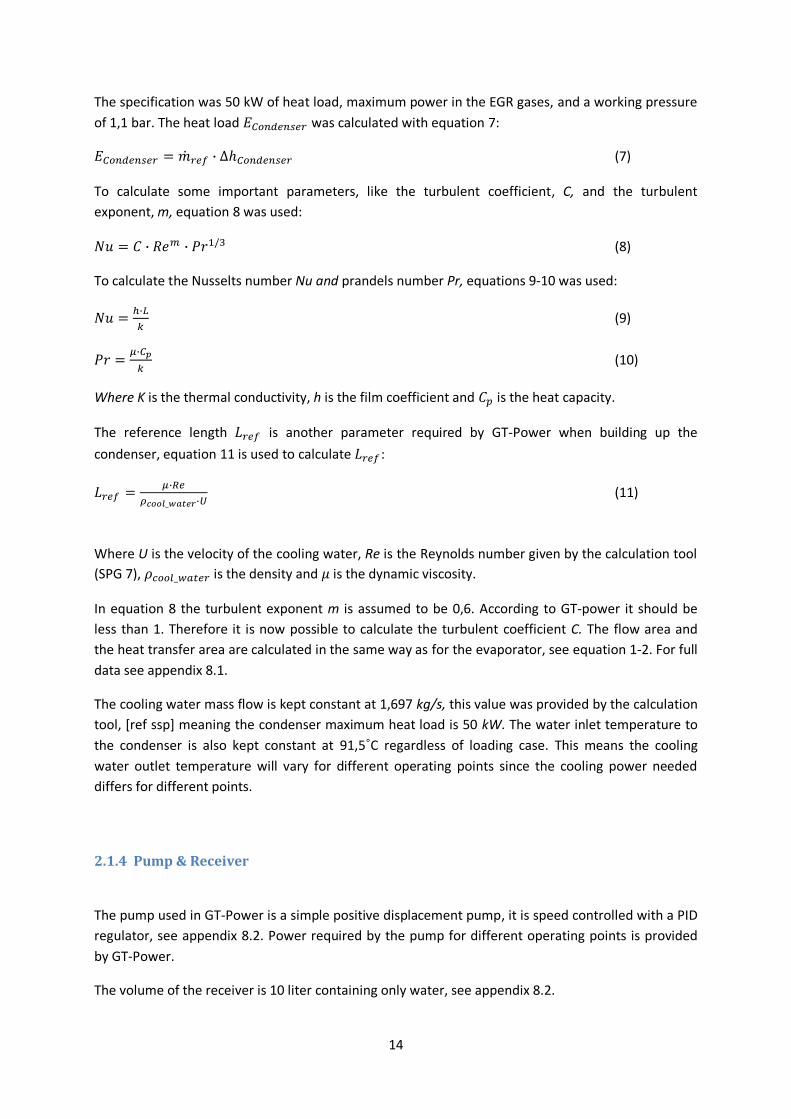
mass flow also means the cooling of the diesel exhaust gases would increase, resulting in more
energy utilized from the exhaust gases, see figure 26. Another interesting fact is the decreasing
margin between the steam temperature and the EGR temperature for lower steam pressures and
lower levels of superheating.
Figure 26. The refrigerant flow versus the EGR-outlet/steam temperature after the evaporator, for
operating point 10
To maximize the power output from the evaporator the steam pressure must be as low as possible
and the steam must be just superheated i.e. highest refrigerant mass flow possible according to the
result above.
During the experimental tests the upper limit of the steam pressure was set to 100 bar. The
evaporator wasn’t tested for higher steam pressures out of safety.
The steam temperature, the refrigerant mass flow and the EGR outlet temperature from the
experimental test are presented in table 3 (see table 1 for full data of the operating points of the ESC
cycle). For EGR inlet temperatures higher than 450 ˚C the water flow is approximately a tenth of the
EGR flow, while for EGR temperatures lower than 300 ˚C the water flow is approximately 3 % of the
EGR flow.
240
260
280
300
320
340
360
380
400
6 7 8 9 10 11 12 13
Tem
pe
ratu
re [˚
C]
Flow [g/s]
100 bar_ EGR
60 bar_ EGR
100 bar_ Steam
60 bar_ Steam
Boil Temp 100 bar
Boil Temp 60 bar

27
Table 3. EGR temperatures and EGR flows for the ESC cycle
Operating point
EGR flow [g/s]
Water flow [g/s]
EGR inlet temperature
[˚C]
EGR outlet temperature
[˚C]
Steam temperature
[˚C]
Steam Pressure
[bar]
Load case [%]
2 77,9 7,9 500 284 329 100 100
3 71,4 4 384 248 282 60 50
4 90,3 6,7 436 274 312 90 75
5 51,7 3,47 416 255 288 60 50
6 66,3 6,4 467 267 310 90 75
7 36,9 1,16 306 193 200 13 25
8 109,8 9,91 483 277 326 100 100
9 60,1 2,14 296 192 217 20 25
10 122,4 10,57 459 275 325 100 100
11 75,7 2,29 290 200 225 20 25
12 111,6 6,7 407 265 308 90 75
13 89,3 3,68 355 248 277 60 50
The 100 % load points were run at a steam pressure of 100 bar, the 75 % load points were run at a
steam pressure of 90 bar , the 50 % load points at 60 bar while the 25 load points were run at highest
possible steam pressure that would result in superheated steam. The steam pressure was chosen so
the full load points would have the highest steam pressure. The steam pressure was then decreased
for the lower loading cases as can be seen in table 3.
The EGR power and the evaporator’s EGR efficiency for the ESC cycle operating points can
be seen in figure 27, the dots representing the 100 % load points, stars present the 75 % load points,
triangles illustrating the 50 % load points and finally the squares stands for the 25 % load cases.
Figure 27. The evaporator’s efficiency based on the EGR cooling
0
10
20
30
40
50
60
70
30 32 34 36 38 40 42 44 46
E EG
R[k
W]
ηEGR [%]
2
3
4
5
6
7
8
9
10
11
12
13

28
The efficiency varies between operating points in the same load case, this is due the different EGR
inlet temperature. Since the strategy was to keep a constant steam pressure and relatively constant
steam temperatures, this means only the refrigerant flow will separate the different operating point
in the same load case, as can be seen in table 3. As mentioned earlier a higher EGR temperature
results in a higher percentage refrigerant flow when comparing EGR flows. For example looking at
the 75 % load case it shows that operating point 6 have efficiency of approximately 45 % while
operating point 4 has 39 % and point 12 has a efficiency of 37 %. Comparing the EGR inlet
temperatures in table 3 shows that they differ by 40-60 degrees in favor for operating point 6, which
means that the steam pressure applied for operating points 4 and 12 is too high. This can also be
seen if analyzing other operating points, for example operating point 7. The efficiency for this point is
approximately 40 % which is larger than several other operating points, even though the EGR
temperature of point 7 is lower. This is due to the steam pressure for point 7 is 13 bar. Compared
with the relatively low EGR temperature the steam pressure is really low.
The evaporator’s efficiency based on the steam temperature is about 30 % higher than the
EGR efficiency shown above. This efficiency describes how good the evaporator is at heating up the
steam while the EGR efficiency describes how good the evaporator is at cooling down the EGR. One
interesting fact is that the points with high EGR efficiency are the points with low steam efficiency.
For example operating point 13 has the lowest EGR efficiency, about 32 %, while the steam efficiency
is about 77 %, which is the highest percentage of the entire ESC cycle, see figure 28.
Figure 28. The evaporator’s efficiency based on the steam temperature
250
300
350
400
450
500
550
60 62 64 66 68 70 72 74 76 78
EGR
Te
mp
erat
ure
[°C
]
ηSteam [%]
2
3
4
5
6
7
8
9
10
11
12
13

29
3.1.1 Transient response
A transient test run was performed to understand the evaporator’s response. The engine speed and
torque was varied according to figure 29, four operating points were run. All the load levels and the
speed levels in the ESC driving cycle were covered as the torque curve and the speed curve indicates.
P1 and P2 is the refrigerant pressure before and after the evaporator, T2-1 and T2-2 is the steam
temperature measured after the evaporator. T-EGR is the EGR inlet temperature while T2-EGR is the
EGR outlet temperature.
Figure 29. The engine, refrigerant and the EGR temperature and flow

30
The change in EGR inlet and outlet temperature and the EGR flow can be seen in figure 29, T-EGR is
the inlet temperature of the EGR and T2-EGR is the outlet temperature of the EGR. Figure 29 also
present the water pressure P1 prior to the evaporator, the steam pressure P2 after the evaporator,
the steam temperature T2-1 -T2-2 after the evaporator and the refrigerant flow. The steam pressure
was chosen as the highest possible pressure resulting in superheated steam. Comparing the x-axis it
is possible to see how “slow/fast” the evaporator is, a change in torque and speed is performed
according to figure 29 one can see how long time after the change in load point is done the steam
takes to settle in. The first change is done after approximately 120 seconds, the steam temperature
and pressure settles in at approximately 200 seconds. This means the process takes about 80
seconds to settle in.
The two thermocouples mentioned in the experimental setup can be seen in figure 30, the margin
between the two is a couple of degrees prior to evaporation (t=0 to t=x1) and during evaporation
(t=x1 to t=x2). Then the difference between them grows to about 10 degrees when all the water is
evaporated and the steam starts to superheat. This means one of the two micro tubes group gets all
the water evaporated before the other group, the steam has lower density meaning it takes more
place. This result in more water shuffled over to the second group, therefore the margin increase
between the two groups.
Although it is important to mention that the difference in degrees lays as maximum 10 degrees,
meaning the refrigerant is still pretty equally distributed.
Figure 30. The two temperature sensors and the pressure before and after the evaporator
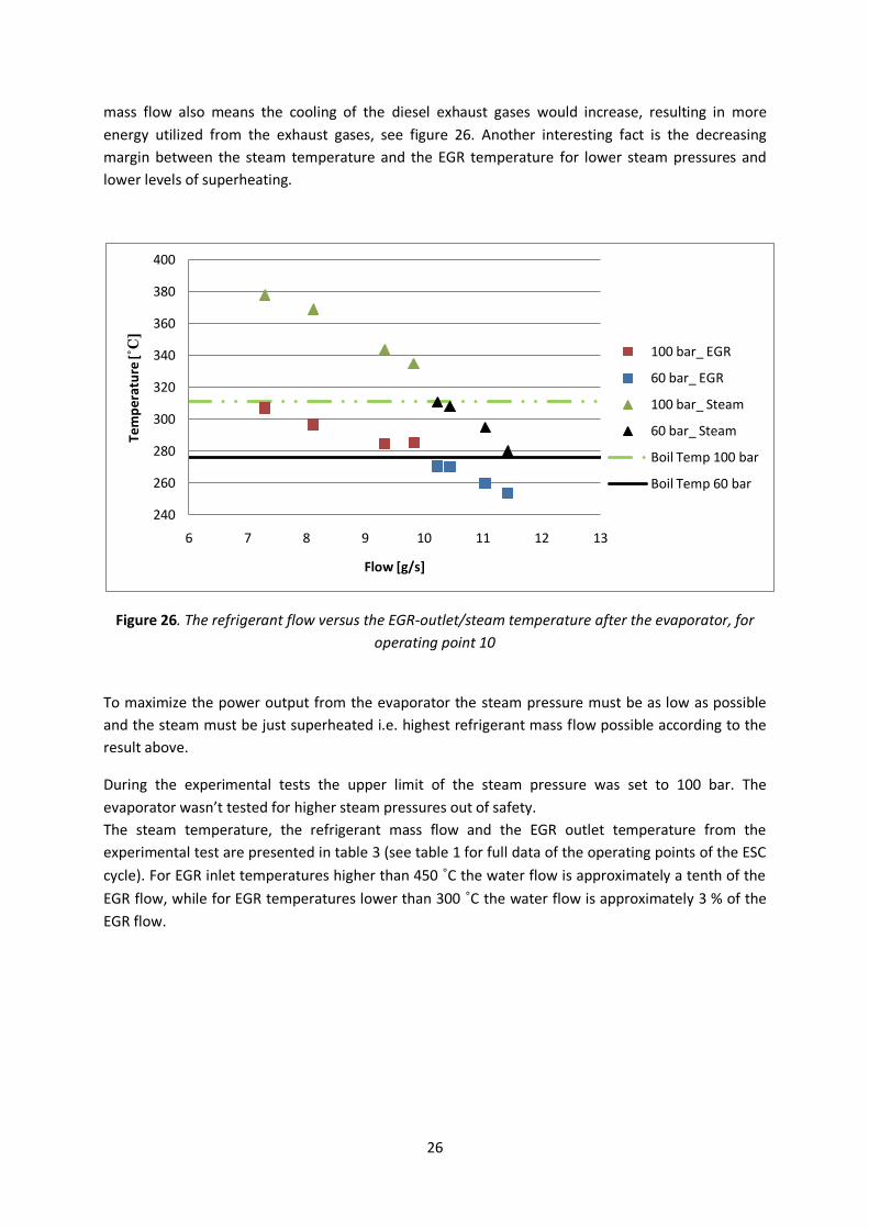
The same thing occurs while analyzing the thermocouples mounted on the micro tubes inside the
evaporator, see figure 31. The difference is a couple of degrees before evaporation starts, but the
margin increases due to evaporation. There are 16 thermocouples but only five of them are
presented. This way it is easier to understand. Thermocouple T_G always has the highest steam
temperature while T_C always gives the lowest steam temperature.
0
50
100
150
200
250
300
350
400
0 50 100 150 200 250
Tem
per
atu
re [˚
C]
Time [sec]
P1
P2
T2-1
T2-2
X1 X2
31
Figure 31. The thermocouples inside the evaporator
During these test the engine load is constant resulting in a constant EGR flow and temperature. The
operating point is 2, see table 1.
50
100
150
200
250
300
350
400
450
0 50 100 150 200 250
Tem
pe
ratu
re [˚
C]
Time [sec]
T_A_'C
T_C_'C
T_G_'C
T_H_'C
T_L_'C
T_N_'C

32
3.2 GT-Power Results
As mentioned earlier a model was developed in GT-Power to simulate the Rankine cycle with
water as the refrigerant. As figure 32 illustrates there is a cooling circuit, an EGR circuit and finally
the refrigerant circuit. In the refrigerant circuit there are four different states, each state is
defined by the pressure P, mass flow and the temperature T. The refrigerant mass flow
is constant i.e. the same mass flow at all states, while is equal to because
water is incompressible.
Figure 32. The rankine layout
The cooling water mass flow to the condenser is kept constant, 1,697 kg/s regardless of load
case, while the inlet temperature is 91,5 C. Regarding the EGR circuit it will be varied in
order to understand the effect of the EGR mass flow and the EGR temperature. Whereas the
cooling pressure is assumed to be 1,5 bar and the EGR pressure is acquired from
the engine test, see table 1.

33
3.2.1 EGR temperature variation
In this simulation the steam pressure and the steam temperature is kept constant, se
table 4.
Table 4. Values of the steam pressure and steam temperature
Parameter Simulation 1 Simulation 2
[bar] 150 90
[˚C] 359 320,5
[˚C] 514-550-600-650-700 514-550-600-650-700
While the EGR pressure and mass flow is also kept constant. The EGR inlet temperature
is varied according to table 4 in this test.
Figure 33. Steam power for different EGR inlet temperatures
As the EGR inlet temperature rises the EGR power input increases, which leads to increased steam
power. This gives more power in the steam entering the piston expander. Analyzing figure 33 also
shows that the steam power is larger for 90 bar, confirming the engine test result. Because the
boiling temperature is lower at 90 bar compared to 150 bar the refrigerant mass flow can be
increased resulting in a higher steam power output after the evaporator.
Studying the expanders output power shows for every 5 kW gain in EGR power the expander power
output increase with approximately 0,8-1 kW. As can be seen in figure 34, the 150 bar line overtake
the 90 bar line for higher EGR inlet temperature despite the steam power input to the expander is
higher for the 90 bar line.
15
20
25
30
35
40
30 35 40 45 50 55
E Ste
am [k
W]
EEGR [kW]
150 bar
90 bar

34
Figure 34. EGR power, steam power and expander power for different EGR temperatures and
refrigerant pressure
This depends on the thermal efficiency of the Rankine cycle, it increases with the steam pressure
according to figure 35. Another explanation is the relationship between the EGR temperature and
the steam pressure as will be shown later in the report. To maximize the power output from the
piston expander the optimal steam pressure needs to be determined. If a low steam pressure is
applied then a large amount of steam power is obtained after the evaporator, but also low thermal
system efficiency. If a very high pressure is applied then the amount of steam power provided by the
evaporator decreases, but a high system thermal efficiency is acquired. So if the energy input is
increased then the optimal pressure should also increase. This can be seen in the growing difference
in terms of the expander’s power output, see figure 34.
3
3,5
4
4,5
5
5,5
6
6,5
7
7,5
15
20
25
30
35
40
45
50
55
500 550 600 650 700 750
E Ste
am [k
W],
EEG
R [k
W]
EGR Temperature [˚ C]
EGR power_150 bar
Steam Power_150 bar
Steam Power_90 bar
EGR Power_ 90 bar
Exp power_150 bar
Exp power_90 bar
E Exp
[kW
]

35
Figure 35. The Rankine thermal efficiency for different steam pressures
Also it is interesting to see the thermal efficiency decreasing when the energy input is growing. This
depends on the fact that the model was calibrated for certain energy input, when the energy input
grow then the expander doesn’t utilize enough energy out of the superheated steam. This can be
observed when analyzing the steam pressure after the expander, see figure 36.
Figure 36. The steam pressure prior to the condenser for different levels of EGR power
To explain the lift in the expander’s output power the evaporator’s efficiency was analyzed, see
figure 37. This shows that increasing the EGR temperature results in higher evaporator efficiency.
Also the 90 bar line have higher efficiency because the boiling temperature is lower and therefore a
16
16,5
17
17,5
18
18,5
19
30 35 40 45 50 55
ηW
HR
[%
]
EEGR [kW]
150 bar
90 bar
1,2
1,3
1,4
1,5
1,6
1,7
1,8
1,9
30 35 40 45 50 55
P4
Ref
[bar
]
EEGR [kW]
150 bar
90 bar

36
higher refrigerant mass flow can be applied leading to a higher steam power.
Figure 37. The efficiency of the evaporator for varying energy inputs
Another interesting observation is that the EGR gases cools down more if the inlet temperature is
increased see figure 38. This depends on the growing refrigerant mass flow, as mentioned earlier the
steam temperature was kept constant so when the energy input is increased the mass flow
also grow. A higher refrigerant mass flow leads to a larger cool down of the EGR gases.
Figure 38. The outlet temperature of the exhaust gases at 150 bar pressure
Higher EGR temperatures can best be obtained through supplementary burning, which means
burning diesel in the exhaust system prior to the evaporator. A calculation has been made to
50
55
60
65
70
75
30 35 40 45 50 55
ηE
GR
[%]
EEGR [kW]
150 bar
90 bar
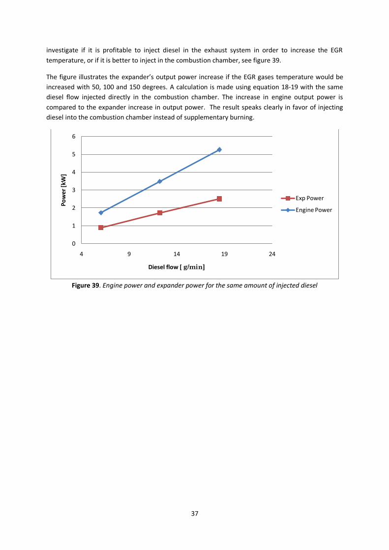
37
investigate if it is profitable to inject diesel in the exhaust system in order to increase the EGR
temperature, or if it is better to inject in the combustion chamber, see figure 39.
The figure illustrates the expander’s output power increase if the EGR gases temperature would be
increased with 50, 100 and 150 degrees. A calculation is made using equation 18-19 with the same
diesel flow injected directly in the combustion chamber. The increase in engine output power is
compared to the expander increase in output power. The result speaks clearly in favor of injecting
diesel into the combustion chamber instead of supplementary burning.
Figure 39. Engine power and expander power for the same amount of injected diesel
0
1
2
3
4
5
6
4 9 14 19 24
Po
we
r [k
W]
Diesel flow [ g/min]
Exp Power
Engine Power

38
3.2.2 EGR Flow variation
The EGR flow was varied and the power output from the expander analyzed, the EGR flow was
varied according to table 5.
Table 5. The EGR flow variation
Simulation Steam pressure [bar] EGR Flow [g/s]
1 150 77,9-90-100-110-120-130
2 90 77,9-90-100-110-120-130
In figure 40 the steam power can be seen as a function of the EGR power. The same logic applies
here as for the EGR temperature variation.
Figure 40. Steam power for several EGR flows and refrigerant pressure
As figure 41 illustrates, if the EGR power is increased with approximately 5 kW then the expander’s
power output is increased with approximately 0,5 kW. Similar to the EGR temperature increase figure
it is possible to see that the 90 bar line result in higher expander power for lower energy input. But
when the energy input grow it is possible to see the 150 bar equal the 90 bar line, as mentioned
earlier if the energy input to the system increases then the optimal steam pressure also increases.
15
17
19
21
23
25
27
29
31
33
35
30 35 40 45 50 55 60
E Eva
p[k
W]
EEGR [kW]
150 bar
90 bar

39
Figure 41. Expander power, EGR power and steam power for different EGR flows
Analyzing the effect of the increased EGR flow on the evaporator’s efficiency is interesting because it
is desirable to understand if this evaporator is over/under dimensioned. As table 5 illustrates the
flow has been raised in several steps. The total increase in EGR flow is 52 g/s, which is an increase
with 67 % of the default EGR flow. Analyzing figure 42 shows that the evaporators efficiency
decrease with approximately 1 % when comparing the original EGR flow with the final value of the
EGR flow for the same steam pressure. If the evaporator would be placed on an engine with larger
EGR flow rate or in the exhaust pipe (not only the EGR), this would mean that the efficiency is
practically the same i.e. this evaporator is over dimensioned for the used DC1306 engine. Also it is
possible to see the difference in efficiency between the two pressure levels, approximately 5 % in
favor of the 90 bar steam pressure level. The difference between 90 bar and 150 bar is the boiling
temperature, it is lower for 90 bar, see figure 4. A lower boiling temperature results in a higher
refrigerant mass flow which leads to a larger cooling of the EGR gases, that means the numerator in
equation 4 grows. This leads to larger evaporator efficiency.
3
3,5
4
4,5
5
5,5
6
6,5
15
20
25
30
35
40
45
50
55
60
65
70 90 110 130 150
E Eva
p[k
W],
EEG
R[k
W]
EGR Flow [g/s]
EGR power_150 bar
Steam Power_150 bar
Steam Power_ 90 bar
EGR Power_90 bar
Exp Power_150 bar
Exp Power_90 bar
E Exp
[kW
]

40
Figure 42. The evaporator’s efficiency for different energy input
3.2.3 Fuel consumption reduction
To understand the impact of such a system analysis has to be made about fuel savings, figure 43
represents the reduction of fuel combustion for several power inputs to the waste heat recovery
system. Increasing the power input is done with two different methods, either through
supplementary firing which leads to higher EGR temperatures or by increasing the EGR rate resulting
in a higher EGR mass flow. Starting from the default settings for operating point 2 and then keeping
the mass flow constant while increasing the temperature a couple of steps and vice versa. The results
clearly shows that the EGR temperature have a bigger impact than the EGR flow. Also it is possible to
decrease the fuel consumption with up to 2,6 % if the EGR temperature is raised approximately 200
degrees, this percentage could increase if the exhaust gases was used instead of only the EGR gases.
Figure 43. Reduction of fuel consumption for different energy inputs, 150 bar
51
52
53
54
55
56
57
58
59
30 35 40 45 50 55 60
ηE
GR
[%]
EEGR [kW]
150 bar
90 bar
1,2
1,4
1,6
1,8
2
2,2
2,4
2,6
2,8
30 35 40 45 50 55 60
RFC
[%
]
EEGR [kW]
EGR Flow
EGR Temprature
41
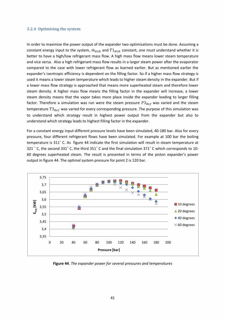
3.2.4 Optimizing the system
In order to maximize the power output of the expander two optimizations must be done. Assuming a
constant energy input to the system, and constant, one must understand whether it is
better to have a high/low refrigerant mass flow. A high mass flow means lower steam temperature
and vice versa. Also a high refrigerant mass flow results in a larger steam power after the evaporator
compared to the case with lower refrigerant flow as learned earlier. But as mentioned earlier the
expander’s isentropic efficiency is dependent on the filling factor. So if a higher mass flow strategy is
used it means a lower steam temperature which leads to higher steam density in the expander. But if
a lower mass flow strategy is approached that means more superheated steam and therefore lower
steam density. A higher mass flow means the filling factor in the expander will increase, a lower
steam density means that the vapor takes more place inside the expander leading to larger filling
factor. Therefore a simulation was run were the steam pressure was varied and the steam
temperature was varied for every corresponding pressure. The purpose of this simulation was
to understand which strategy result in highest power output from the expander but also to
understand which strategy leads to highest filling factor in the expander.
For a constant energy input different pressure levels have been simulated, 40-180 bar. Also for every
pressure, four different refrigerant flows have been simulated. For example at 100 bar the boiling
temperature is 311˚ C. As figure 44 indicate the first simulation will result in steam temperature at
321 ˚ C, the second 331˚ C, the third 351˚ C and the final simulation 371˚ C which corresponds to 10-
60 degrees superheated steam. The result is presented in terms of the piston expander’s power
output in figure 44. The optimal system pressure for point 2 is 120 bar.
Figure 44. The expander power for several pressures and temperatures
3,35
3,4
3,45
3,5
3,55
3,6
3,65
3,7
3,75
0 20 40 60 80 100 120 140 160 180 200
E Exp
[kW
]
Pressure [bar]
10 degrees
20 degrees
40 degrees
60 degrees

42
As mentioned earlier the thermal efficiency of a Rankine cycle is proportional to the steam pressure,
which means a higher pressure results in higher thermal efficiency, see figure 45. Higher level of
superheating result to a higher system efficiency compared with a lower level of superheating. In
order to acquire a higher steam temperature the refrigerant flow must be reduced. This means lower
pump power and steam power as shown earlier. Since the WHR efficiency takes the pump- and
steam -power into consideration, see equation 15, this leads to a higher efficiency compared to just
superheating the steam. But the disadvantage is the decreased steam power entering the expander,
compared to the just superheated steam, leading to a lower power output from the expander, see
figure 46.
Figure 45. The thermal efficiency of the system at different pressures and temperatures
Still the highest expander power is not acquired at 180 bar (see figure 44), this depends on the steam
power before the expander, see figure 46.
Figure 46. Steam power in front of the expander
14
15
16
17
18
19
20
21
0 50 100 150 200
ηW
HR
[%]
Pressure [bar]
10 degrees
20 degrees
40 degrees
60 degrees
15
16
17
18
19
20
21
22
23
0 20 40 60 80 100 120 140 160 180 200
E Ste
am[k
W]
Pressure [bar]
10 degrees
20 degrees
40 degrees
60 degrees

43
As figure 46 shows highest steam power is obtained at the lowest pressure, this depends on the
boiling temperature. Because of the low boiling temperature the mass flow can be increased. Also it
is possible to see that roughly superheated steam result in highest power output from the
evaporator.
As described earlier the expander is replaced by a speed regulated turbine in GT-Power, this means
that the turbines speed reveals the filling factor i.e. if the turbines speed increases when the filling
factor increases and vice versa. Analyzing figure 47 shows that a higher pressure level gives a lower
filling factor which would mean higher isentropic efficiency. Also it is possible to see that the margin
between the different levels of superheated steam decrease with higher steam pressure. But as
figure 44 shows the best power output from the expander is obtained at 120 bar for the lowest level
of superheated vapor, this means it is best to run with lowest level of superheated vapor. If taking
the higher isentropic efficiency, for higher steam pressures, into account as a function of filling factor
the optimal operating pressure will increase some. In this study the isentropic efficiency has been set
to a constant value of 65 %. The dependence of the filling factor has not been considered.
Figure 47. The expander speed for several refrigerant pressure and temperatures
The second optimization of this system is to decide the optimal steam pressure for different EGR
inlet temperatures. Optimal steam pressure is the pressure that results in the highest power output
from the expander. It is known that low steam pressures results in the largest steam power output
from the evaporator but at the same time with higher steam pressure a higher system thermal
efficiency is acquired. Therefore a simulation was run with varied steam pressure for different EGR
inlet temperature, see appendix 8.3 for full result. As can be seen in figure 48 the steam pressure
should be chosen depending on the EGR inlet temperature, a higher temperature leads to higher
steam pressure.
0
1000
2000
3000
4000
5000
6000
7000
8000
9000
10000
0 20 40 60 80 100 120 140 160 180 200
Spe
ed
[R
PM
]
Pressure [bar]
10 degrees
20 degrees
40 degrees
60 degrees

44
Figure 48. Optimal steam pressure for different EGR inlet temperature
3.2.5 The ESC driving cycle
In this chapter several operating points from table 1 will be presented. The simulation strategy was
to decide the steam pressure with the help of figure 48 while the level of superheating is chosen to
10 degrees superheated steam according to the result. This should result in maximizing the power
output from the expander.
The steam power for the different operating points can be seen in table 6, as mentioned earlier a
higher EGR temperature result in higher steam pressure. The highest steam pressure that results in
superheated vapor is chosen for operating point 9, 25 % load case, this doesn’t necessarily mean the
optimal pressure, meanwhile the highest steam pressure is 120 bar for operating point 2. The highest
refrigerant flow is 11,2 g/s for point 10. The pressure drop of the refrigerant is 7,9 bar for the highest
mass flow.
Table 6. The refrigerant properties
Operating point
Steam Power [kW]
Steam pressure [bar]
Refrigerant Flow [g/sec]
Refrigerant Pressure
drop [bar]
Steam Temperature
[˚C]
2 19,2 120 8,15 6,25 335
3 11,5 40 4,7 4,4 260
4 18,2 60 7,46 5,77 286
6 15,9 90 6,56 5,19 313
8 25,1 90 10,39 7,9 313
9 5,2 18,3 2,19 2,9 222
10 27,25 80 11,21 8 305
12 19,9 50 8,13 6,23 274
13 12,5 30 5 4,48 244
300
350
400
450
500
550
0 20 40 60 80 100 120 140
EGR
-Te
mp
era
ture
[˚ C
]
Pressure [bar]

45
In table 7 it is possible to see how much of the steam power that is extracted by the expander. Also
the system efficiency is presented, as can be seen in tables 6-7 a higher steam pressure result in
higher WHR efficiency. Finally the reduction in fuel consumption is presented for the corresponding
operating point. Operating point 10 stands for the largest saving with 1,7 % at the actual engine load
case.
Table 7. Illustrates required/obtained power of the different components for several operating points
Operating point
Pump Power [kW]
Expander Power [kW]
WHR Efficiency [%]
RFC [%]
2 0,26 3,72 18,4 1,46
3 0,05 1,8 15,2 1,31
4 0,12 3,1 16,4 1,48
6 0,158 2,93 17,4 1,51
8 0,259 4,53 17 1,65
9 0,013 0,78 14,7 1,15
10 0,25 4,77 16,6 1,7
12 0,115 3,22 15,6 1,55
13 0,043 1,78 13,9 1,31
The EGR power input to the evaporator can be seen in table 8. The EGR power varies from 12 kW, 25
% load case, to 50 kW, 100 % load case. The EGR cools down only 82 degrees for point 9. This
depends on the low EGR inlet temperature but also the low refrigerant flow. The EGR pressure drop
is the pressure drop over both the evaporator and EGR cooler.
Table 8. Presents the cooling of the EGR and EGR power for several operating points
Operating point
T-EGR [˚C] ∆T EGR
[˚C]
EGR Flow [g/s]
EGR Pressure Drop [bar]
EGR Power [kW]
2 514 227 77,9 0,78 36,16
3 385 148 71,4 0,3 22,6
4 434 186 90,3 0,6 33,6
6 478 221 66,3 0,5 28,3
8 474 211 109,8 0,8 46,1
9 295 82 60,1 0,04 12
10 463 205 122,4 0,82 49,9
12 411 164 111,6 0,55 38,7
13 360 126 89,3 0,35 25,9
The cooling power required is illustrated in table 9, it varies from 4,5 kW up to 21,8 kW. The
temperature and pressure of the condenser can also be seen in table 9. For example, the pressure
differs with 0,4 bar when comparing point 10 and 9. This is due to the filling factor in the expander,
for the full load point the volume flow rate is much higher than for the 25 % load point. This results in
higher condenser pressure for point 10 since the expander doesn’t utilize enough energy of the
superheated steam.

46
Table 9. The temperature and pressure of the condenser, the cooling power for several operating
points
Operating point
Condenser Temperature
[˚ C]
Condenser Pressure
[Bar]
T1Ref
[˚C]
P1Ref
[bar] Cooling
Power [kW]
2 108,1 1,35 103 1,3 15,3
3 106,4 1,27 102 1,26 9,6
4 107,8 1,33 103 1,31 14,8
6 106,9 1,29 102 1,26 12,6
8 110,9 1,48 104 1,42 20
9 102 1,1 100 1,1 4,5
10 112,1 1,54 105 1,47 21,8
12 108,9 1,38 103 1,35 16,3
13 106 1,25 102 1,24 10,4
Figure 49 represents the T-S diagram for operating point 2. In stage (A) the refrigerant is in liquid
state just ahead of the evaporator. While stages (B)-(D) illustrates the refrigerant heat up until it
reach the boiling point, evaporating and finally superheating in the evaporator. Stage (E) represents
the expansion phase. At the end of the expansion the refrigerant is in two phase state, 15 % water
and 85 % steam in this case. The final stage (F) represents the condenser where the refrigerant
leaving the condenser is only in liquid form and sub cooled by two degrees, see also figure 1 and
figure 5 for better understanding.
Figure 49. T-S diagram for operating point 2
50
100
150
200
250
300
350
400
450
0 2000 4000 6000 8000 10000
Series1
Saturation Curve

47
3.2.6 Exhaust flow
This simulation represents the case where an evaporator would be mounted in the exhaust pipe,
after the turbine. This means a larger exhaust flow, compared with the EGR flow. The disadvantage is
the low exhaust temperatures since they cool down 80-150 degrees compared to the EGR
temperatures. This simulation was performed for three different operating points from the ESC cycle.
The power, pressure, temperature and the flow of the steam can be seen in table 10. The optimal
steam pressure is 30 bar for operating point 2 according to figure 48. The level of superheating is
increased since just superheated steam didn’t work in the model. This is because of the big change in
the energy input which the model is not calibrated for. As for the steam pressure for operating points
3-4, the lowest working pressure is applied since there is no data in this master thesis for the optimal
steam pressure for low exhaust/EGR temperature. The same evaporator used in the EGR loop is now
placed in the exhaust pipe, considering the large increase in the exhaust mass flow the evaporator is
under dimensioned leading to a decreasing efficiency.
Table 10. The refrigerant properties
Operating point
Steam Power [kW]
Steam pressure [bar]
Refrigerant Flow [g/sec]
Refrigerant Pressure
drop [bar]
Steam Temperature
[˚C]
2 34,7 31,8 13,6 8,7 280
3 18,2 22 7,3 5,4 240
4 31,96 23,8 12,5 8,4 270
The expander power is increased for all the three points compared to only the EGR as an energy
input, this leads to increased reduction of the fuel consumption.
Table 11. Illustrates required/obtained power of the different components
Operating point Pump Power [kW] Expander Power [kW]
WHR Efficiency [%]
RFC [%]
2 0,13 4,74 13,3 1,95
3 0,047 2,35 12,68 1,73
4 0,099 4,38 13,39 2,14
Table 12 illustrates the exhaust gas properties, as can be seen the highest exhaust gas temperature is
360 ˚C while the exhaust mass flow is much higher than the EGR flows. This results in increased
exhaust power input energy to the system. The evaporator’s efficiency ηExhaust is based on how much
power it utilizes from the exhaust, it can be seen in table 12. The exhaust evaporator efficiency
ηExhaust for operating point 2 is 20 % lower than the EGR evaporator efficiency ηEGR, see figure 37. As
learned earlier the evaporator’s efficiency increases if the steam pressure decreases, since the
refrigerant flow can be increased leading to more energy utilized from the exhaust/EGR power. The
steam pressure in the exhaust pipe is about 30 bar while 90 bar in the EGR pipe. This means that the
evaporator is highly under dimensioned.
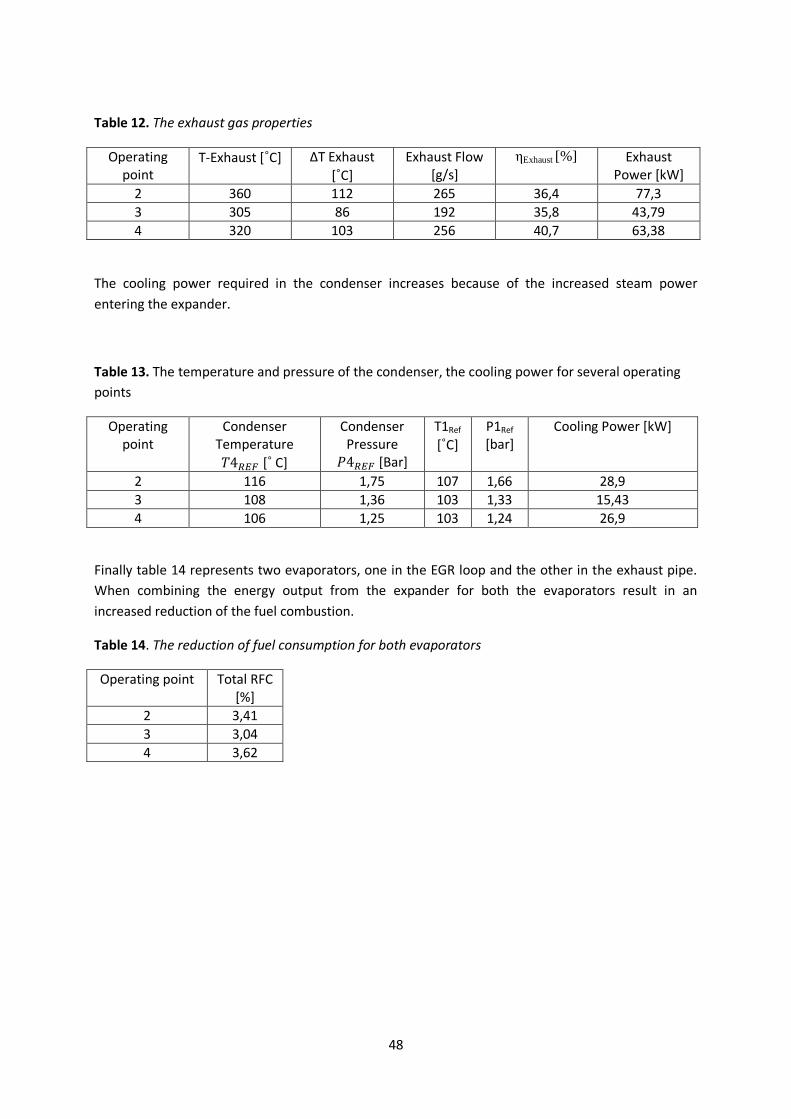
48
Table 12. The exhaust gas properties
Operating point
T-Exhaust [˚C] ∆T Exhaust
[˚C]
Exhaust Flow [g/s]
ηExhaust [%] Exhaust Power [kW]
2 360 112 265 36,4 77,3
3 305 86 192 35,8 43,79
4 320 103 256 40,7 63,38
The cooling power required in the condenser increases because of the increased steam power
entering the expander.
Table 13. The temperature and pressure of the condenser, the cooling power for several operating
points
Operating point
Condenser Temperature
[˚ C]
Condenser Pressure
[Bar]
T1Ref
[˚C]
P1Ref
[bar] Cooling Power [kW]
2 116 1,75 107 1,66 28,9
3 108 1,36 103 1,33 15,43
4 106 1,25 103 1,24 26,9
Finally table 14 represents two evaporators, one in the EGR loop and the other in the exhaust pipe.
When combining the energy output from the expander for both the evaporators result in an
increased reduction of the fuel combustion.
Table 14. The reduction of fuel consumption for both evaporators
Operating point Total RFC [%]
2 3,41
3 3,04
4 3,62

49
3. Discussion
If one just looks at the evaporator the strategy should be low steam pressure and just
superheated steam i.e. high refrigerant mass flow. This would result in the largest steam power
after the evaporator, according to figures 25 and 46.
The purpose is to achieve a high output power from the expander, but with the strategy
mentioned above this will not happen. As figure 45 indicate the system thermal efficiency rise
with increasing steam pressure, therefore a high steam pressure is preferable. The disadvantage
is the decreased steam power from the evaporator. Therefore an optimum needs to be found
where the power output from the evaporator and the thermal efficiency at the prevailing steam
pressure results in the largest power obtained from the expander. Figure 44 shows the optimal
pressure for the operating point.
Assuming a constant steam pressure the superheating degree has to be decided in order to
obtain the largest expander power. If one only looks at the evaporator at a constant steam
pressure, roughly superheated vapor would lead to the highest power output, see figure 44. One
disadvantage is the increased cooling power needed, the same logic applies at the condenser as
for the evaporator i.e. higher refrigerant flow results in higher cooling power. Analyzing figure 47
though shows that the expander speed i.e. filling factor is lower for the roughly superheated
vapor, but also that the margin is decreasing for higher steam pressures. This means for even
higher pressures, up to 250 bar the larger level of superheated steam may have a lower expander
speed if the trend remains. Looking at figure 44 clearly suggest that the optimal pressure is way
lower than 250 bar, which should mean that the optimum level of superheating is precisely
superheated steam. The issue is the constant isentropic efficiency used for the expander, again if
one looks at figure 47 one discovers that the speed of the expander is lower for higher steam
pressures. This means that isentropic efficiency of the expander is higher for higher pressure,
which could result in lifting the optimal steam pressure in figure 44.
If the optimal steam pressure would increase to say 250 bar, following the trend in figure 47
would suggest higher isentropic efficiency for the larger level of superheating.
Therefore it is crucial to determine a relationship between the expanders speed and the
isentropic efficiency in order to acquire more accurate results.
Studying figures 35 and 42 clearly speaks in the favor of the EGR temperature over the EGR flow,
for every 5 kW increase in the EGR power 0,5 kW is obtained from the expander if the source of
the rise was the EGR flow. While the double is obtained if the input energy lift was caused by the
EGR temperature. Therefore it is favorable to increase the EGR temperature, but looking at figure
40 shows that it is better to use the required diesel flow needed to increase the EGR
temperature a desired amount of degrees directly in the combustion chamber, rather than
supplementary burning.
Figure 49 shows the EGR temperature versus the optimal steam pressure. Higher EGR
temperature i.e. higher energy input result in higher optimal steam pressure which is logical.
Because higher energy input to the system results in the possibility to increase the steam
pressure and acquire a higher system thermal efficiency while still getting a reasonable power

50
output from the evaporator. This leads to larger power output from the expander at a higher
steam pressure. This is also confirmed by figures 34 and 41, when increasing the energy input to
the system, the 150 bar line equals/overtakes the 90 bar line. Initially the optimal pressure is
closer to 90 bar but as the energy input grows the steam pressure rises closer or even passes the
150 bar line resulting in the 150 bar line overtaking the 90 bar line in terms of expander power.
Also the difference between the EGR temperature and the EGR flow is visible in this case, as an
increase in EGR temperature clearly pushes the optimal pressure higher than the corresponding
EGR flow. That’s the reason why the 150 bar line overtakes the 90 bar line, in the EGR
temperature figure, while the 150 bar line only equals the 90 bar line in the EGR flow figure.
For a constant flow figures 23 and 24 shows that the heat transfer is larger at lower steam
pressure but the evaporator works better at higher steam pressures. The heat transfer from the
exhaust gases is smaller at a higher steam pressure compared to a lower but the steam outlet
temperature is still higher meaning the performance of the evaporator is better at higher
pressures. Looking only at the evaporator the magnitude of the applied steam pressure is not
important if the refrigerant mass flow is constant, since the difference in terms of output power
is negligible. If one looks at the whole system then it is desirable to apply as high pressure as
possible in order to raise the thermal efficiency of the system.
The reduction of fuel consumption is approximately 1,4 % in operating point 2, see figure 43. If
the EGR power is increased 10 kW the reduction of fuel consumption will rise with approximately
0,2 %, if the EGR flow was the reason of the lift in EGR power. If the EGR temperature is the
cause in the change in EGR power then a 5 kW lift result in 0,3 % improvement of the fuel
consumption.
The evaporator manufactured by Ranotor is over dimensioned for this specific engine (DC1306).
Increasing the EGR flow with approximately 67 % resulted in 1 % decrease in the evaporator’s
efficiency, see figure 42. While increasing the EGR temperature lifted the evaporator’s EGR
efficiency , see figure 37. This depends on that the same amount of EGR flow enters the
evaporator, but with higher temperature i.e. more energy. In the case of increased EGR flow, the
mass flow entering the evaporator increases leading to less cooling of the EGR gases, due to lack
of heat exchange areas.
The reduction of fuel consumption lays between 1,1-1,7 % for most of the ESC cycle operating
points. This percentage could be increased either by using the entire exhaust gases instead of
only the EGR gases. For example operating point 2 reduces the fuel consumption with 3,4 %, see
table 14. The highest cooling power required by the condenser is about 21 kW for operating
point 10, since the EGR cooling is no longer needed some power is saved and could instead be
used to condense the vapor. If the required cooling power is too high, more than the engines
cooling capacity, one could opt to run that specific operating point with a high level of
superheating, this leads to a reduced cooling power demand from the condenser.
Figure 49 shows that at the end of expansion state the refrigerant is in the two phase area. As
mentioned earlier for a piston expander this is no problem. The water percentage is 20 % as a
maximum for all the simulated points in the ESC cycle. Assuming a constant energy input to the
system i.e. constant operating point, then the water percentage increases with the steam
pressure. As figure 47 reveals the filling factor of the expander decreases with higher steam

51
pressures, meaning a larger percentage of water. Assuming there is a requirement of having
superheated steam after the expansion phase, the solution would be to increase the level of
superheating in the evaporator. The water percentage is about 10 % lower for the 60 degrees
level of superheating compared to the 10 degrees level of superheating, this is for a full load
operating point.

52
4. Conclusion
The steam pressure should be depending on the EGR temperature, a higher EGR temperature means
a higher steam pressure. The steam should be roughly superheated in order to obtain the largest
power output from the expander. Since the condenser is water cooled and the cooling power is
obtained from the engine it could happen, probably at full load, that the engine power is not enough
to condense the steam. At this situation the superheating level should be increased resulting in a
reduced cooling power required by the condenser.
Supplementary burning is a method used to increase the EGR inlet temperature by injecting fuel in
the exhaust pipe, resulting in increased power input to the system which leads to higher power
obtained from the expander. Calculations show that it is better to inject the diesel directly into
combustion chamber since the power output from the engine is larger for the same diesel flow.
The water mass flow is very low, 20 g/s as a maximum, which means the receiver in the GT-Power
model is too large. The volume is 10 liter, considering the low refrigerants mass flow indicates that
the receiver could be downsized.
In order for this WHR system to be profitable the entire energy in the exhaust gases must be used i.e.
not only the EGR as the case was in this master thesis. Especially when analyzing point 9, 25 % load
point, only 0,8 kW is obtained from the expander. Therefore it is crucial to use all the exhaust energy
in order to push up this number.
The WHR system is best suited in application where the engine loading case is not varied too much.
Since heavy duty trucks engines and marina engines often travel long distances and the engine
loading case is not varied too much the WHR system is a good option in order to utilize the energy in
the exhaust gases. The WHR system is a more challenging solution for inner city driving.
53
5. Future work
A master thesis where the primary goal is to build a model of a piston expander in GT-Power and
customize the isentropic efficiency curve as a function of the expanders filling factor. Thereafter
connect the piston expander, instead of the turbine, to the model and investigate if the current
result still agrees. Also mount the piston expander downstream the evaporator and run some
experimental result. Then compare the experimental results with the simulation result to validate the
model.
Build an evaporator with bigger heat exchange area in GT-Power, in order to avoid having an under
dimensioned evaporator. This leads to increased power output from the expander meaning larger
reduction in fuel consumption, when compared to the current results.
Compare water to other refrigerant in order to understand if water is a sufficient working fluid.

54
7. References
[1] http://www.gtisoft.com/
[2] N. Hanna, H. Achkoudir et al., ”Waste Heat Recovery,” Kungliga Tekniska Högskolan, 2010
[3] http://en.wikipedia.org/wiki/Rankine_cycle
[4] Hans Jonsson, “Applied Thermodynamics- Collection of Formulas,”
Stockholm, March 1997
[5] Teng, H., Regner, G. and Cowland, C., “Waste Heat Recovery of Heavy-Duty Diesel Engines by
Organic Rankine Cycle Part II: Working Fluids for WHR-ORC,”
SAE Paper, No.2007-01-0543, 2007
[6] Ho Teng and Gerhard Regner, “Improving Fuel Economy for HD Diesel Engines with WHR Rankine
Cycle Driven,”
SAE Paper, No 2009-01-2913, 2009
[7] http://www.ranotor.se/index1.html
[8] I. Ekroth and E. Granryd, “Tillämpad termodynamik,”
KTH, Stockholm 1994
[9] Rasmus Löfstrand Grip, “A mechanical model of an axial piston machine,”
Licentiate Thesis in Machine Design, 2009
[10] Peter Platell, “Displacement expanders for small scale cogeneration,”
ISSN 1100-5335, TRITA-MAK 1993:1
[11] http://www.swep.net/index.php?tpl=page0&lang=en&id=411

55
8. Appendix
8.1 Condenser Data
CONDENSER - Performance
Condenser: B200Tx30
Fluid Side 1 : Steam
Fluid Side 2 : Water
Flow Type : Counter-Current
Table 15. The heat load, inlet- and outlet temperature of the condenser
DUTY REQUIREMENTS Side 1 Side 2
Heat load kW 50,00
Inlet temperature °C 110,00 88,00
Condensation temperature (dew) °C 101,85
Subcooling K 2,00
Outlet temperature °C 99,86 95,00
Flow rate kg/s 0,02196 1,697
Fluid condensed kg/s 0,02196
Max. pressure drop kPa 50,0 50,0

56
Table 16. Pipe diameters, Reynolds number and operating pressure
PLATE Condenser Side 1 Side 2
Total heat transfer area m² 3,61
Heat flux kW/m² 13,8
Mean temperature difference K 10,14
O.H.T.C. (available/required) W/m²,°C 6340/1370
Pressure drop -total* kPa 0,845 16,7
- in ports kPa -0,0282 0,290
Operating pressure - outlet kPa 107
Number of channels 14 15
Number of plates 30
Oversurfacing % 364
Fouling factor m²,°C/kW 0,575
Port diameter mm 60,0 53,0
Recommended inlet connection diameter mm From 42,2 to 94,5
Recommended outlet connection diameter mm From 1,71 to 5,41
Reynolds number 3070
Inlet port velocity m/s 12,3 0,798
Table 17. Physical properties of the condenser
PHYSICAL PROPERTIES Side 1 Side 2
Reference temperature °C 101,86 91,50
Liquid - Dynamic viscosity cP 0,277 0,309
- Density kg/m³ 957,0 964,4
- Heat capacity kJ/kg,°C 4,220 4,209
- Thermal conductivity W/m,°C 0,6796 0,6759
Vapor - Dynamic viscosity cP 0,0123
- Density kg/m³ 0,6269
- Heat capacity kJ/kg,°C 1,973
- Thermal conductivity W/m,°C 0,02529
- Latent heat kJ/kg 2,252
Film coefficient W/m²,°C 16300 14600
Average wall temperature °C 99,52 98,57
Channel velocity m/s 5,23 0,246
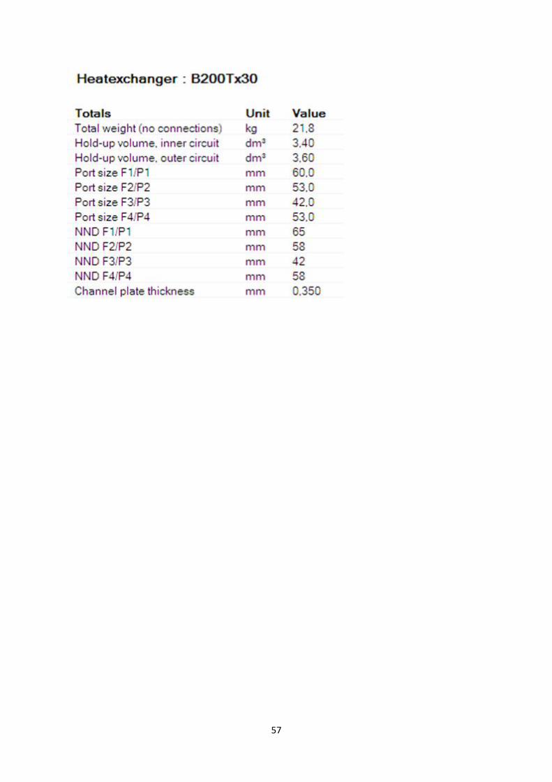
57

58
8.2 Pump, Expander & Reciever
Component Isentropic efficiency [%]
Volumetric efficency [%]
Template name in GT-Power
Pump 40 80 PumpPosDispRefrig
Expander 65 70 TurbPosDispRefrig
Reciever - - RecieverDryerRefrig
8.3 GT-Power results
In this section the simulation results for the other operating points in the ESC cycle are presented.
8.3.1 EGR temperature variation
The following results are for operating point 12 in the ESC cycle.
Figure 50. The steam power and EGR power for two steam pressures
10
15
20
25
30
35
40
45
50
30 35 40 45 50 55 60 65 70
E Ste
am [k
W]
EEGR [kW]
150 bar
90 bar

59
Figure 51. The expander power, steam power and the EGR power for two different steam pressures
Figure 52. The pressure ahead of the condenser
2
3
4
5
6
7
8
9
10
20
30
40
50
60
70
400 450 500 550 600 650 700
E Ste
am [k
W],
EEG
R [k
W]
EGR Temperature [°C]
EGR power_150 bar
EGR power_90 bar
Steam power_150 bar
Steam power_90 bar
Exp power_150 bar
Exp power_90 bar
E Exp
[kW
]
1
1,2
1,4
1,6
1,8
2
2,2
2,4
30 35 40 45 50 55 60 65 70
P4 R
ef [b
ar]
EEGR [kW]
90 bar
150 bar

60
Figure 53. The reduction in fuel consumption for two different steam pressures
8.3.2 EGR flow variation
The following results are for operating point 12 in the ESC cycle.
Figure 54. EGR power and steam power for operating point 12
1
1,5
2
2,5
3
3,5
4
4,5
30 35 40 45 50 55 60 65 70
RFC
[%
]
EEGR [kW]
150 bar
90 bar
10
12
14
16
18
20
22
24
26
30 35 40 45 50 55
E Ste
am [k
W]
EEGR [Power]
150 bar
90 bar

61
Figure 55. EGR power, steam power and expander power for two different steam pressures
Figure 56. The reduction in fuel consumption for two different steam pressures
2
2,5
3
3,5
4
4,5
5
10
15
20
25
30
35
40
45
50
55
100 120 140 160 180
E Ste
am
[kW
], E
EG
R [k
W]
EGR Flow [g/s]
Steam power_150 bar
Steam power_90 bar
EGR power_150 bar
EGR power_90 bar
Exp power_150 bar
Exp power_90 bar
E Exp
[kW
]
1
1,2
1,4
1,6
1,8
2
2,2
2,4
30 35 40 45 50 55
RFC
[%
]
EEGR [kW]
150 bar
90 bar

62
8.3.4 Optimizing the system
The result for operating points 3, 4, 6, 8, 10, 12 and 13 are presented in figures 57-69 below.
Figure 57. Expander power for several steam pressures, point 8
Figure 58. The thermal efficiency of the system for different steam pressures, point 8
4
4,1
4,2
4,3
4,4
4,5
4,6
30 50 70 90 110 130 150 170 190
E Exp
[kW
]
Pressure [bar]
10 degrees
20 degrees
40 degrees
60 degrees
1515,5
1616,5
1717,5
1818,5
1919,5
20
0 50 100 150 200
ηW
HR
[kW
]
Pressure [bar]
10 degrees
20 degrees
40 degrees
60 degrees

63
Figure 59. The steam power for different pressures, point 8
Figure 60. The expander speed for different steam pressures, point 8
Figure 61. The expander power, steam power and system efficiency for different pressures, point 10
17
19
21
23
25
27
29
31
20 40 60 80 100 120 140 160 180 200
E Ste
am [k
W]
Pressure [bar]
10 degrees
20 degrees
40 degrees
60 degrees
1000
3000
5000
7000
9000
11000
13000
20 40 60 80 100 120 140 160 180 200
Spee
d [R
PM
]
Pressure [bar]
10 degrees
20 degrees
40 degrees
60 degrees
4,45
4,5
4,55
4,6
4,65
4,7
4,75
4,8
0
5
10
15
20
25
30
35
0 50 100 150 200
E Ste
am [k
W],
ηW
HR
[%
]
Pressure [bar]
10 degrees_Steam
10 degrees_Efficiency
10 degrees_ExpanderE Exp
[kW
]

64
Figure 62. The expander power, steam power and system efficiency for different pressures, point 6
Figure 63. The expander power, steam power and system efficiency for different pressures, point 4
Figure 64. The expander power, steam power and system efficiency for different pressures, point 12
2,5
2,55
2,6
2,65
2,7
2,75
2,8
2,85
2,9
2,95
3
10
11
12
13
14
15
16
17
18
19
20
20 40 60 80 100 120 140
E Ste
am [k
W],
ηW
HR
[%
]
Pressure [bar]
10 degrees_Steam
10 degrees_Efficiency
10 degrees_Expander
E Exp
[kW
]
2,8
2,85
2,9
2,95
3
3,05
3,1
3,15
12
13
14
15
16
17
18
19
20
21
22
0 20 40 60 80 100 120 140
E Ste
am [k
W],
ηW
HR
[%
]
Pressure [Bar]
10 degrees_Steam
10 degrees_Efficiency
10 degrees_Expander
E Exp
[kW
]
2
2,2
2,4
2,6
2,8
3
3,2
3,4
12
14
16
18
20
22
24
0 20 40 60 80 100 120 140 160
E Ste
am[k
W],
ηW
HR
[%
]
Pressure [bar]
10 degrees_Steam
10 degrees_Efficiency
10 degrees_Expander
E Exp
[kW
]

65
Figure 65. Expander power for several steam pressures, point 3
Figure 66. Steam power for several steam pressures, point 3
Figure 67. The system efficiency for different steam pressures, point 3
1,4
1,45
1,5
1,55
1,6
1,65
1,7
1,75
1,8
1,85
20 30 40 50 60 70 80 90 100 110
E Exp
[kW
]
Pressure [bar]
10 degrees
20 degrees
40 degrees
60 degrees
6
7
8
9
10
11
12
13
20 30 40 50 60 70 80 90 100 110
E Ste
am
Pressure [bar]
10 degrees
20 degrees
40 degrees
60 degrees
12
13
14
15
16
17
18
19
0 20 40 60 80 100 120
ηW
HR
[%
]
Pressure [bar]
10 degrees
20 degrees
40 degrees
60 degrees

66
Figure 68. The expanders speed for different steam pressures, point 3
Figure 69. The expander power, steam power and system efficiency for different pressures, point 13
0
1000
2000
3000
4000
5000
6000
7000
20 30 40 50 60 70 80 90 100 110
Spe
ed
[RP
M]
Pressure [bar]
10 degrees
20 degrees
40 degrees
60 degrees
0
0,2
0,4
0,6
0,8
1
1,2
1,4
1,6
1,8
2
6
8
10
12
14
16
18
20
0 20 40 60 80 100 120
E Ste
am [k
W],
ηW
HR
[%
]
Pressure [bar]
10 degrees_Steam
10 degrees_Efficiency
10 degrees_ExpanderE Exp
[kW
]
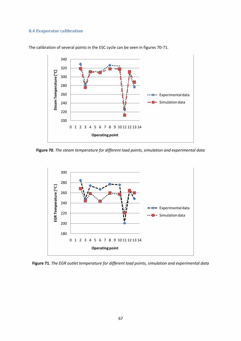
67
8.4 Evaporator calibration
The calibration of several points in the ESC cycle can be seen in figures 70-71.
Figure 70. The steam temperature for different load points, simulation and experimental data
Figure 71. The EGR outlet temperature for different load points, simulation and experimental data
200
220
240
260
280
300
320
340
0 1 2 3 4 5 6 7 8 9 10 11 12 13 14
Ste
am T
em
pe
ratu
re [°
C]
Operating point
Experimental data
Simulation data
180
200
220
240
260
280
300
0 1 2 3 4 5 6 7 8 9 10 11 12 13 14
EGR
Te
mp
erat
ure
[°C
]
Operating point
Experimental data
Simulation data


