How Access to Credit Affects Self-Employment: Differences by Gender during India’s Rural Banking Reform Nidhiya Menon, Brandeis University Yana van der Meulen Rodgers, Rutgers University Version: August 31, 2009 Corresponding author: Yana van der Meulen Rodgers, Women’s and Gender Studies Department, Rutgers University, New Brunswick, NJ 08901. Tel 732-932-9331, fax 732-932- 1335, email [email protected]. Contact information for Nidhiya Menon: Department of Economics & IBS, MS 021, Brandeis University, Waltham, MA 02454-9110. Tel 781-736-2230, fax 781-736-2269, email [email protected]. We thank Ghazala Mansuri and participants at the 2009 World Bank and University of Michigan Conference on Female Entrepreneurship. Thanks also to Rachel McCulloch for her detailed comments and suggestions. We acknowledge Ksenia Rogalo for her capable research assistance. This research is supported by the World Bank and by a Rutgers University Research Council Grant.
Transcript
How Access to Credit Affects Self-Employment:
Differences by Gender during India’s Rural Banking Reform
Nidhiya Menon, Brandeis University
Yana van der Meulen Rodgers, Rutgers University
Version: August 31, 2009
Corresponding author: Yana van der Meulen Rodgers, Women’s and Gender Studies
Department, Rutgers University, New Brunswick, NJ 08901. Tel 732-932-9331, fax 732-932-
1335, email [email protected]. Contact information for Nidhiya Menon: Department of
Economics & IBS, MS 021, Brandeis University, Waltham, MA 02454-9110. Tel 781-736-2230,
fax 781-736-2269, email [email protected]. We thank Ghazala Mansuri and participants at
the 2009 World Bank and University of Michigan Conference on Female Entrepreneurship.
Thanks also to Rachel McCulloch for her detailed comments and suggestions. We acknowledge
Ksenia Rogalo for her capable research assistance. This research is supported by the World Bank
and by a Rutgers University Research Council Grant.
1
How Access to Credit Affects Self-Employment:
Differences by Gender during India’s Rural Banking Reform
Abstract: This study uses a pooled sample of household survey data collected by India’s
National Sample Survey Organization between 1983 and 2000 to examine the impact of access
to credit on self-employment among men and women in rural labor households. Results indicate
that access to credit encourages women’s self-employment as own-account workers and
employers, while it discourages men’s self-employment as unpaid family workers. Additional
results indicate that ownership of land, a key form of collateral, serves as one of the strongest
predictors of men’s and women’s self-employment. There are also interesting class differences
within the bottom tier of India’s caste system: self-employment is less likely for members of
scheduled castes, but more likely for members of scheduled tribes.
Keywords: Women, India, Asia, Self-Employment, Loans, Rural Banks
2
I. Introduction
Microenterprises constitute an important source of productive employment for men and
women around the world. While some individuals start their own businesses as a means toward
greater flexibility in generating income and new opportunities for innovation, others resort to
self-employment in microenterprises as a coping strategy in the face of scarce employment
opportunities. Especially in developing countries where the very poor are more constrained in
their economic choices by the market environment, lack of infrastructure, and insufficient
sources of affordable credit, small-scale entrepreneurship serves as one of the primary vehicles
for income generation (Banerjee and Duflo 2007). In addition, women use self-employment as a
means of combining employment with childcare responsibilities. Household business ventures
often employ a substantial proportion of the workforce, particularly in less developed countries
with large informal sectors. Understanding the conditions under which people decide to operate
household enterprises can contribute to policy reforms that support self-employed individuals
and promote other such entrepreneurial activities.
A key area of policy intervention is the provision of small-scale loans through
microfinance and rural banks. Both have aided in reducing poverty by providing a diverse range
of financial services to the poor and the disenfranchised. While the Self Employed Women’s
Association (SEWA) in India and the Bangladesh Rural Advancement Committee (BRAC) and
Grameen Bank in Bangladesh have received an enormous amount of attention in scholarly and
policy discourse, other institutions in developing countries have also experimented with a
number of financial sector reforms to provide pecuniary resources to people without access to
conventional loans from commercial banks. An important example is India’s rural social banking
program, which was initialized following the nationalization of banks in 1969. This state-led
3
expansion of the banking sector focused primarily on opening new bank branches in previously
unbanked rural locations and was demonstrated by Burgess and Pande (2005) to have led to a
statistically significant reduction in poverty in rural India.
Our objective in this research is to examine whether greater access to financial resources
increased the likelihood of self-employment, and whether there were differences in effects along
gender lines. Since self-employed households tend to be less poor, if greater access to finances
increased self-employment probabilities, then this is one possible channel through which India’s
social banking program may have worked to reduce poverty. As noted in Das (2003), the extent
of rural self-employment varies by social affiliation, religion, and gender. In addition, the ten-
year period following bank nationalization saw a tremendous increase in the agricultural labor
force, which rose by a third for women (16 to 21 million) and almost 10 percent for men (32 to
34 million) (Bennett 1992). This study conducts a detailed examination of the determinants of
self-employment for men and women using combined micro-data and macro-data sources that
span the years 1983 to 2000. Following the classification in the National Sample Survey
Organization (NSSO) schedules, we denote the self-employed to be individuals who worked as
own-account workers and unpaid family workers.
We find that India’s rural banking reform program increased the likelihood of women’s
self-employment as own-account workers, while having little effect on men’s self-employment
work as own-account workers. A possible explanation is that since women have restricted
access to formal employment in developing countries such as India, when the household obtains
a loan, it is rational for women to become self-employed and to start a home-based business.
This explanation finds resonance in the conclusions of Luke and Munshi (2007), who argue that
underprivileged groups in society are much more likely to avail of new opportunities. Our
4
finding that the credit expansion had relatively stronger effects for women contributes to an
expanding literature, but one with conflicting results, on the impact of credit on economic
activity in developing countries.
Background
In India's rural areas, a substantial proportion of income is subject to crop-cycle
fluctuations that result from seasonality and unexpected weather patterns. Seasonality coupled
with the lack of access to formal insurance mechanisms implies that poor rural households can
undergo marked fluctuations in their annual incomes. Absent sources of income that do not
depend on weather outcomes, these fluctuations in income flows can not only affect household
consumption patterns, but also decisions about employment. Greater access to credit through
microfinance programs and rural banking facilities can improve the ability of households to
withstand shocks to consumption and production (Menon 2006).
In response to this potential role for credit in the rural sector and the inadequate coverage
then provided by existing formal credit and savings institutions, India’s government made a
concerted effort to increase the number of banks throughout rural India. In what Burgess and
Pande (2005) describe as the biggest bank expansion agenda followed by the government of any
country, India embarked on an aggressive program to increase opportunities for poor households
in the rural sector to acquire credit and deposit savings in formal institutions. Between 1969,
when the government nationalized India’s commercial banks, and 1990, when the official
licensing program (described in detail below) ended, approximately 30,000 new bank branches
opened in previously unbanked rural locations. The program included mandates based on
population and stock of branches per capita, with a particularly ambitious licensing reform in
5
1977 that required banks to open branches in four previously unbanked locations in order to
obtain a license to open a branch in a location that already had banks.
Not only did the government encourage branch openings in unbanked rural locations, it
also controlled deposit and lending policies so as to provide individuals with incentives to use
the new banks. It set savings rates above those in urban areas and lending rates below those of
urban areas. Additional provisions set targets on lending in priority areas that included
agriculture and small-scale entrepreneurs. After the program ended in 1990, no additional bank
branches were opened in unbanked rural locations (Burgess and Pande 2005). However, rural
banking activity continued to grow throughout the 1990s; total bank branches, commercial bank
deposits in the rural sector, and commercial bank advances in the rural sector all continued to
expand (Figure 1).
The increased availability of finance described above may mitigate circumstances that
tend to make women’s work in self-employment less productive and profitable. For example,
since much of rural female labor in India is uneducated and restricted in geographic mobility,
women are likely to be self-employed in “female” trades, which tend to be small-scale and only
marginally profitable (spinners, weavers, and makers of tobacco products). In this context,
improved access to credit may have provided the opportunity for female workers to move up the
ladder of self-employment activities and to undertake more profitable work in larger-scale
operations. Although we do not have the data on profits or number of employees hired in a self-
employment business to formally test this assertion, we can examine occupational patterns over
time to assess the extent to which credit may have facilitated shifts to more productive and
profitable work.
6
To this end, Figures 2 and 3 present descriptive statistics for men and women for the
most common occupational categories among the self-employed with and without loans in 1983
and in 1999-2000. The most common occupation for men and women was cultivators (owners).
The dominance of land cultivation as the primary occupation was particularly true for the self-
employed with no loans. While men showed more variation in other leading occupational
categories between 1983 and 2000, livestock farming and dairy farming consistently ranked high
for women (especially women with loans). Although these descriptive results are simple
correlations, they are consistent with the hypothesis that for women, credit can facilitate the
move from cultivation toward more capital-intensive livestock and dairy farming. A final point
of interest is the steady rise of bidi making as a leading occupation among rural self-employed
women during the 1990s, especially for women with no loans. Producing these hand-rolled
cigarettes is a highly labor-intensive process in an industry comprised of both factory-based and
home-based enterprises. The predominance of women with no loans in bidi production is
consistent with the low capital requirements in this industry.
A growing body of research has examined the effects of increased access to credit on
economic activity in low-income countries, with a range of sometimes contradictory findings.
For example, Pitt and Khandker (1998) found that credit given to female participants in Grameen
programs had strong positive effects on both male and female labor supply. Also evaluating the
effects of the Grameen bank as well as the Bangladesh Rural Advancement Committee (BRAC),
Hashemi et al. (1996) conclude that participants mostly used the loans for small-scale self-
employment in activities as diverse as rice-paddy processing, animal husbandry, and artisan
crafts. These programs increased women’s control over finances, raised women’s economic and
social standing, and boosted women’s productivity in and out of the home. Other research shows
7
that credit and non-credit services made available by participation in BRAC and Grameen
programs led to positive profits from self-employment (McKernan 2002), and that the presence
of village-level microfinance groups in Thailand stimulated asset growth and occupational
mobility (Kaboski and Townsend 2005).1
In contrast to these positive results, an experimental approach in de Mel et al. (2008)
showed that small cash or in-kind grants given to a randomly-selected group of microenterprises
in Sri Lanka resulted in high rates of return for men, on the order of about 5 percent per month,
but no positive returns for female-owned enterprises. Coleman (1999) finds that several group-
lending programs for women in Northeast Thailand had no statistically significant impact on a
number of measures of economic activity, including production, sales, and time spent working.
In a set of more nuanced results, Kevane and Wydick (2001) find that among those entrepreneurs
who borrowed from a microenterprise lending institution, women entrepreneurs of child-bearing
age were unsuccessful in creating employment with their businesses compared to other
entrepreneurs, but there were no gender differences in business sales following credit provision.
Finally, McKenzie’s (2009) review of a recent set of randomization trials lends support to the
argument that simply providing greater access to capital is not sufficient to help microenterprises
grow. McKenzie’s assessment of microenterprises and finance in developing countries concludes
that additional policies designed to improve business training, provide business-development
services, and facilitate shifts into more profitable sectors are likely to enhance the impact of
credit on small business ventures.
Methodology and Data
Our analysis examines the probability of engaging in self-employment, conditional on a
household’s access to credit and a set of other personal and household characteristics. Again, the
8
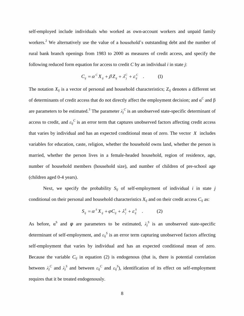
self-employed include individuals who worked as own-account workers and unpaid family
workers.2 We alternatively use the value of a household’s outstanding debt and the number of
rural bank branch openings from 1983 to 2000 as measures of credit access, and specify the
following reduced form equation for access to credit C by an individual i in state j:
)1(.C
ij
C
jijij
C
ij ZXC
The notation Xij is a vector of personal and household characteristics; Zij denotes a different set
of determinants of credit access that do not directly affect the employment decision; and αC and β
are parameters to be estimated.3 The parameter λj
C is an unobserved state-specific determinant of
access to credit, and εijC is an error term that captures unobserved factors affecting credit access
that varies by individual and has an expected conditional mean of zero. The vector X includes
variables for education, caste, religion, whether the household owns land, whether the person is
married, whether the person lives in a female-headed household, region of residence, age,
number of household members (household size), and number of children of pre-school age
(children aged 0-4 years).
Next, we specify the probability Sij of self-employment of individual i in state j
conditional on their personal and household characteristics Xij and on their credit access Cij as:
)2(.S
ij
S
jijij
S
ij CXS
As before, αS and φ are parameters to be estimated, λj
S is an unobserved state-specific
determinant of self-employment, and εijS is an error term capturing unobserved factors affecting
self-employment that varies by individual and has an expected conditional mean of zero.
Because the variable Cij in equation (2) is endogenous (that is, there is potential correlation
between λjC and λj
S and between εij
C and εij
S), identification of its effect on self-employment
requires that it be treated endogenously.
9
To estimate the model, we use a pooled sample comprised of four cross-sections of
household survey data collected by the NSSO. The data include the years 1983 (38th
round),
1987-1988 (43rd
round), 1993-1994 (50th
round), and 1999-2000 (55th
round). For each round,
we utilize the “Activity” file of the Employment and Unemployment module - Household
Schedule 10 - which contains detailed information on individual and household socioeconomic
characteristics for an average of about 643,000 individuals in each year. To construct our
working sample, we retain all working-age individuals (ages 18-59) living in rural households
classified as agricultural labor and other labor households. We restrict our analysis to rural labor
households since information on household loan activity in the NSSO data is available only for
these types of households. A final selection criterion involves keeping only households in India’s
16 largest geographical states for which data on rural bank branch openings are available (these
16 states are as in Burgess and Pande (2005)). These restrictions leave us with a total of 408,385
observations in the pooled sample.
Sample statistics in Table 1 indicate that about 14 percent of working-age men and
women residing in rural labor households report being self-employed as their primary economic
activity. While there is no gender difference in the likelihood of being self-employed, men and
women do differ in the type of self-employment they pursue: about a tenth of self-employed men
versus almost half of self-employed women are unpaid family workers. Table 1 also shows that
more than 80 percent of women had never received schooling during the period, compared to
about 60 percent of men. Interestingly, more than 40 percent of men and women belong to the
lowest tier of India’s class system: the scheduled castes and scheduled tribes (also known as
backward castes). A comparison of these statistics with other types of rural households indicates
a relatively high representation of uneducated adults and of the lowest-tier social classes in our
sample. Table 1 further indicates that the vast majority of men and women are Hindu, married,
10
and land owners, with a heavier concentration in southern and central states compared to other
regions of India. Women are much more likely to live in female-headed households compared to
men (11 percent versus 3 percent), while there is not much of a substantive difference between
the characteristics of women and men in other types of living arrangements shown. Reflecting
the social norm that related households reside together, the average household size is between
five and six people, one of whom is often a young child.
To examine how rural banks affect the decision to be self-employed, we merge the
employment data with a set of credit variables from the NSSO data files on household loan
activity for the same households for 1983, 1987-88, 1993-94, and 1999-2000. The credit
variables provide detailed information on loans and debt, including the source and purpose of the
loans as well as the value of outstanding debt. Sample means indicate that close to 40 percent of
working-age adults in rural labor households in every year have at least one outstanding loan,
and the average household loan size is about 4000 rupees in real terms. The data indicate a strong
reliance by households on different types of loans: the loans are more than twice as likely to be
cash-based loans rather than in-kind and other types of loans, and households with current loans
are about three times as likely to have obtained their loan from an informal source (including
employers, landlords, moneylenders, shopkeepers, relatives, and friends) as from a formal source
(including the government (both national and state), co-operative societies, and banks). Also of
note is the purpose of outstanding debt: about 60 percent of households with current loans have
used their loans for consumption, 25 percent have used them for production, and the remaining
15 percent have used their loans for other purposes such as debt repayment. Such diversification
of credit sources and uses is not specific to India’s rural sector. Previous evidence for Madras,
one of India’s largest cities, indicates that the majority of women who had obtained a loan at a
11
relatively low interest rate from a credit network had also obtained an informal high-interest loan
from a money lender (Noponen 1991). Similar to rural laborers in the NSSO data, Noponen finds
that credit recipients in Madras used the loans not only to generate income, but also to smooth
consumption and to repay outstanding loans obtained from money lenders.
Our alternative measure of access to credit is new rural bank branches in previously
unbanked locations. We merge the employment sample with the macro-level database on rural
bank branch openings constructed by Burgess and Pande (2005) for their study on India’s
banking reform. These data cover India’s 16 largest states from 1961 to 2000. The variables
include the number of rural bank branches in previously unbanked locations, total bank branches,
other measures of financial development, measures of population density, measures of state
income, and the number of rural locations in a state (locations in a state are classified as rural on
the basis of population numbers and other criteria).
Credit is endogenous for several reasons, including that individuals with higher
unobserved ability may be more able to obtain loans and also more likely to engage in self-
employment activities. Furthermore, if policy requires that new rural bank branches be placed in
areas that are relatively poor, then estimates of the effects of loan activity may also be biased. As
discussed in Menon (2006), the use of state-level fixed effects, which capture systematic
differences across states in such attributes as average interest rates, aids in removing some of the
bias. We instrument for possible self-selection and non-random bank branch placement using the
trend-reversals that resulted from the Central Bank of India’s imposition and subsequent removal
of the 1:4 licensing requirement (as in Burgess and Pande 2005).4 To improve access to bank
credit in rural India, the Central Bank mandated a new 1:4 licensing policy in 1977 whereby a
bank could obtain a license to open a branch in a location where other branches already existed
12
only if it opened four branches in a rural location where no other branch previously existed. This
requirement remained in place until 1990. Before this policy was implemented in 1977, banks
tended to locate in rich areas with high measures of financial development in order to maximize
profits. With the imposition of this licensing policy in 1977, the rate of branch expansion
increased more rapidly than before in rural poor areas with low measures of financial
development. After 1990, the trend was again reversed, with greater expansion in areas that were
more developed. The difference of the 1977-1990 and post-1990 trends from the pre-1977 trend
in the correlation between a location’s initial measure of financial development and bank branch
expansion in rural areas form our set of instruments for rural bank branch placement.
Burgess and Pande (2005) provide evidence that these trend-reversals were statistically
significant determinants of rural branch openings in previously unbanked locations. We test that
these reversals had no direct effects on self-employment probabilities by analyzing the impact of
the trend-reversals on exogenous covariates that could influence self-employment, including
different categories of education, land ownership, caste, and religion. These test results are
presented in Appendix Table 1. The high p-values for the F-tests in this table indicate that in all
cases we cannot reject the null hypothesis that the sum of the interacted trend variables is zero.
That is, there is no evidence of trend-reversals in control variables that could affect self-
employment, our dependent variable. The absence of such trend sequences in possibly
confounding variables, along with evidence in Burgess and Pande (2005) that the switches in
trends are statistically significant, indicate that the trend-reversals constitute a valid set of
instruments for analyzing bank branch placement. Location specific initial measures of financial
development that influence bank branch placement are also valid instruments for loans obtained
by rural labor households (see Burgess et al. 2005). Hence we use these initial measures of
13
financial development interacted with year dummies as instruments for loans obtained by rural
labor households.
In estimating equations (1) and (2), our analysis employs four procedures. First, we use
probit models to examine the determinants of self-employment and how they differ for men and
women. Next, we add measures of household loan activity to a set of “naïve” probit equations for
self-employment that treat credit exogenously in order to obtain a benchmark estimate for
responsiveness to credit. The coefficients obtained from these naïve estimates underline the
importance of treating credit endogenously. Next, we add the Burgess and Pande measures of
rural bank branch openings to the self-employment equations for men and women and estimate a
set of instrumental-variables probit estimations. Finally, we use the Burgess and Pande variables
to instrument for household loan activity in the self-employment regressions, again using
instrumental-variables probit models. To test for instrument validity, we report p-values from
Sargan’s over-identification test (1958).
Estimation Results
Determinants of Self-Employment: Individual and Household Characteristics
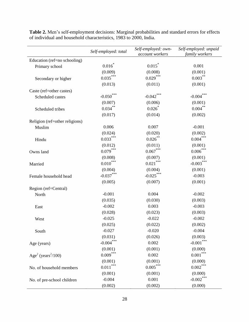
The estimation results begin with findings from the base regressions for the likelihood of
self-employment regressed on the complete set of individual and household characteristics using
the pooled 1983 to 2000 sample. The marginal probability estimates for men are reported in
Table 2 and for women in Table 3, with all variables set at their means in the calculations of the
self-employment probabilities. In both tables, marginal probabilities are reported for overall self-
employment (column one), self-employment as an own-account worker (column two), and self-
employment as an unpaid family worker (column three). Results indicate that for men, the
likelihood of self-employment as own-account workers depends positively on education; the
14
same is true for men’s self-employment as unpaid family workers, but the relationship is not
nearly as strong. For example, the probability of self-employment as own-account workers was
0.03 points higher for men with secondary education and 0.02 points higher for men with
primary education compared to men with no education. However, the probability of self-
employment as unpaid family workers was 0.003 points higher for men with secondary
education but measured imprecisely for men with primary education compared to men with no
education.
Caste and religion also play an important role in predicting men’s self-employment,
although in contrasting ways. While men in the scheduled caste group are 0.05 percentage points
less likely to be self-employed compared to men in higher tiers of the caste system, men in the
scheduled tribes category are about 0.03 percentage points more likely to be self-employed. The
direction of this result holds for both own-account self-employed workers and unpaid family
workers, but the magnitudes are larger for own-account workers. In India, policy makers often
treat the scheduled castes and scheduled tribes as a single category, so these differing effects are
unlikely to be caused by differing policies toward the two groups. Anecdotal evidence suggests
that members of scheduled tribes have some prior experience with home-based work producing
artisan- and cottage-industry goods. This argument is supported by findings in Kijima (2006) that
scheduled tribes, often found living in more remote areas than scheduled castes, have relatively
limited access to infrastructure, irrigation and communication facilities, and employment
opportunities in their villages. Thus, it is likely that scheduled tribes as a group rely more on
their own labor skills to make a living, and are thus more likely to be self-employed. The
scheduled tribes are also known for their seasonal migration, particularly to areas with markets to
produce income by selling their crafts. In contrast, members of scheduled castes tend to be
15
pressured by members of upper castes to remain in their traditional occupations. Therefore,
members of scheduled castes are often employed by others, as opposed to owning and operating
their own businesses (Vaid 2007).
Religion also yields a contrasting relationship, with men of Hindu backgrounds having a
0.03 point higher probability of self-employment and Muslim men showing no statistically
significant difference compared to men with other religious backgrounds. Results further show
that land ownership is one of the strongest predictors of men’s self-employment: the probability
of self-employment is 0.08 points higher for men who live in households that own land
compared to those who do not, with most of this result coming from men’s self-employment as
own-account workers. Finally, being married and having a larger household are positively
associated with men’s self-employment, while living in a female-headed household and age have
a negative association.
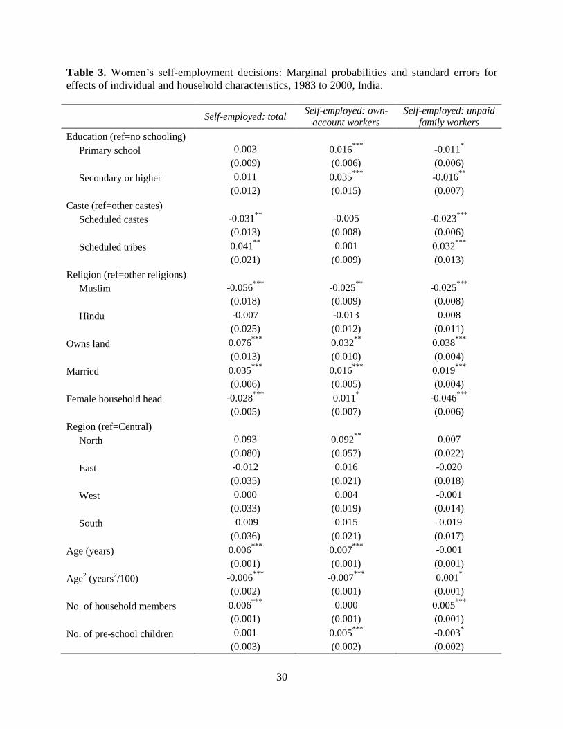
Many of these conclusions also hold for the likelihood of women’s self-employment,
although there are some nuances. Having an education is not as important an indicator of overall
self-employment for women compared to men, mostly because education acts in opposing ways
in affecting women’s self-employment as own-account workers and as unpaid family workers.
We see a strong positive effect for women’s self-employment as own-account workers, where
the probability of self-employment is 0.04 points higher for women with secondary education
and 0.02 points higher for women with primary education compared to women with no
education. However, these coefficient estimates are somewhat smaller in absolute value and take
on the opposite sign in decisions to become unpaid family workers. Like men, women show
strong and interesting differences across caste in the likelihood of self-employment: women in
scheduled castes are 0.03 percentage points less likely to be self-employed compared to women
16
in other castes, and women in scheduled tribes are 0.04 percentage points more likely to be self-
employed. Most of this caste effect is coming from self-employment as unpaid family workers.
Religion operates differently for women compared to men, with being Muslim serving as
a very strong negative predictor of women’s work as own-account workers as well as unpaid
family workers, and Hinduism having no statistically significant influence on self-employment.
As with men, a household’s land ownership is one of the most important predictors of women’s
self-employment. The probability of being self-employed increases 0.08 points for women who
live in households that own land. Interestingly, being married is a positive predictor of both types
of self-employment for women, while marriage decreases men’s probability of engaging in self-
employment as unpaid family workers. Also in contrast to men, women are more likely to
become self-employed as they age. Living in a female-headed household has a large negative
impact on the likelihood of self-employment as unpaid family workers, which appears to drive
the negative effect for overall self-employment. While living in larger households raises the
likelihood that women will be unpaid family workers, those living with a child of pre-school age
are more likely to work as own-account workers.
Household Loan Activity: “Naïve” Probits
The analysis continues by examining the effect of household loan activity on the self-
employment decision using the NSSO loan data merged with the NSSO employment files.
Results for men and women are reported in Table 4, where data are pooled from 1983 to 2000.
Each reported coefficient and standard error is obtained from a separate probit estimation. We
refer to these as the “naïve” probits as they do not instrument for household loans. Results for
men in Table 4 indicate that total loans, formal loans, informal loans, and loans taken for
production purposes all have strong positive effects on self-employment. Such effects persist
17
when self-employment is disaggregated into its components of own-account workers and unpaid
family workers, although magnitudes are in general larger for own-account workers.
Results for women mirror those for men, with the magnitudes of the loan coefficients
again larger for own-account workers compared to unpaid family workers. The repercussions of
India’s rural bank expansion program are expected to appear in the formal loan category; the
naïve estimates in Table 4 suggest that the bank expansion had slightly bigger marginal effects
on male self-employed as compared to female self-employed workers. However, these
implications change when household loans are treated endogenously, as demonstrated below.
Self-Employment and Rural Bank Expansion: Instrumental Variables
In this section, we provide evidence for the impact of credit on employment by merging
the pooled sample of NSSO rural labor households with the Burgess and Pande (2005) state-level
data on the number of bank branch openings in previously unbanked rural locations. The number
of new bank branches is an alternative measure of credit availability with variation across states
and over time.5 To correct for non-random branch placement, we instrument using the trend-
reversals discussed above and in Burgess and Pande (2005). To control for the aggregation bias
that may result from combining individual-level data and state-level data in a single regression,
we report clustered standard errors in all models. The presence of individual and aggregated
right-hand-side regressors causes a downward bias in the estimated standard errors of variables
measured at the state level, which leads to an upward bias in the precision attributed to their
coefficient estimates. By adjusting the standard errors for correlations, we avoid aggregation bias
(Moulton 1990).
Results are reported in Table 5. The most striking result is that women’s self-employment
responds positively to the number of new rural bank branches, and this result is coming entirely
18
from self-employment as own-account workers. In particular, women’s self-employment as own-
account workers rises by 0.16 percentage points following a unit increase in the number of
branches opened in rural unbanked locations per capita. In contrast, men’s self-employment
shows no statistically significant response to new bank branches. The second line of Table 5
indicates that from 1961 to 1990, an additional point of initial financial development reduced
men’s self-employment totals by 0.01 percentage points annually. All results for men and
women include regional and year dummies as well as other controls at the macro and micro
levels.
Another way to address aggregation bias is to use a common level of aggregation in all
regressors. As a robustness check for our results in Table 5, we used state-level data to
implement the instrumental-variables approach. We aggregated the NSSO employment data by
state, year, and gender, and merged these with the state-level data on new bank branch openings.
Because the rural bank data covered 16 states and we had only 4 years of NSSO data aggregates
(1983, 1987-88, 1993-94, and 1999-2000), we effectively had a total of 64 observations for each
of the male and female state-level regressions. We constructed several measures of self-
employment at the state level, including the average probability of engaging in self-employed
work for men and women; the proportion of women among all self-employed individuals; and
other measures that compared whether self-employed individuals were own-account workers,
employers, or unpaid family workers. The estimations tested the relationship between these
alternative state-level aggregated measures of self-employment and bank branch openings using
the trend-reversal variables as instruments, along with state-level controls for religion, caste,
education, and land; year dummy variables to capture year-specific fixed effects; and state
dummy variables to capture state-specific fixed effects. A large number of specification tests that
19
varied and limited the number of control variables yielded mostly insignificant coefficients,
leading us to the conclusion that our limited number of observations yielded too few degrees of
freedom for us to implement this approach successfully.
Self-Employment and Household Loans: Instrumental Variables
In the final set of tests, we employ the trend-reversal approach to instrument for
household loan activity. In particular, we use a measure of financial development in 1961
(number of bank branches per capita) interacted separately with a 1987 year dummy, a 1993 year
dummy, and a 1999 year dummy, to instrument for household loan activity. This approach
follows that in Burgess et al. (2005). We measure household loan activity using four alternative
continuous variables. The first measure is the total nominal value of a loan. The next two loan
variables represent nominal values of loans from formal sources and from informal sources, and
the final loan variables represent nominal values of loans used for production purposes. In all
four measures, individuals who live in households with no loans are assigned a value of zero for
the loan variables. In order for the instrumental-variables probit models to achieve convergence,
we had to use a 50 percent random sub-sample of our pooled data.
Table 6 reports the results. Each reported coefficient and standard error is obtained from
a separate instrumental-variables probit estimation that includes individual characteristics
(education, owns land, and female household head), state dummies, and year dummies as control
variables. The most striking overall results in Table 6 are the strong positive response of
women’s self-employment as own-account workers to having a loan and the strong negative
response of men’s self-employment as unpaid family workers to loan access. For three of the
four measures of loan activity, the probability of women’s self-employment depends positively
and significantly on the loan amount, while the relationship between men’s self-employment as
20
own-account workers and loan activity is small (or even negative) and statistically insignificant.
For example, the probability of women’s self-employment as an own-account worker rose by
0.102 points for a 10 percent change in total loans, compared to no statistically significant
change for men. In contrast, the probability of men’s self-employment as an unpaid family
worker fell by 0.065 points for a 10 percent change in total loans, compared to virtually no
change for women.
The difference between men and women is especially pronounced for formal loans from
banks and for loans used for production purposes. Interestingly, women’s probability of self-
employment as own-account workers shows greater responsiveness to loans from banks
compared to loans from informal sources such as moneylenders, employers, and family
members.6
Discussion and Policy Implications
This paper has examined the role of personal characteristics, household factors, and
access to credit as determinants of self-employment in India’s rural labor households from 1983
to 2000. We measure access to credit in two ways: the indebtedness of rural labor households in
the NSSO data, and the increase in the number of new bank branches in previously unbanked
rural locations that resulted from the Central Bank of India’s nationalization of banks and the
new licensing policy. Results obtained from instrumental variables probit estimations point to a
pronounced difference between men and women in the responsiveness of self-employment
probabilities to credit: formal bank loans and loans targeted for production purposes have a
substantially stronger positive impact on women’s likelihood of being self-employed as own-
account workers compared to men. Furthermore, whereas such loans significantly reduce the
probability of men’s self-employment as unpaid family workers, they have little effect on
21
women’s work under this category. This conclusion about the positive responsiveness of
women’s self-employment as own-account workers to credit also holds when credit is measured
at a more aggregate level as the number of new bank branches in previously unbanked rural
locations. Such benefits to women from formal banking could be explained by the fact that since
they have restricted access to formal employment as compared to men, with the availability of
loans, it is rational for them to start a home-based business.7 Increases in women’s likelihood of
self-employment as own-account workers may also have provided the required flexibility to ease
the path for men’s transition in other occupations.
It is well-documented that employment in home-based enterprises reduces vulnerability
and improves social security. Hence, at the grass-roots level, the greater outreach in rural finance
afforded by India’s nationalization of banks and the 1:4 licensing policy benefitted women by
increasing their probability of engaging in gainful self-employment beyond unpaid family work.
Our findings emphasize the importance of credit in helping people to earn a livelihood from their
own trade or business. As noted in Bennett (1992: 31), “Credit is, in a sense, the gateway to
productive self-employment.”
One of our most striking results from the analysis of self-employment determinants
related to class differences within the lowest tier of India’s social class system. For both men and
women, belonging to a scheduled caste reduced the likelihood of becoming self-employed while
belonging to a schedule tribe increased it. Moreover, land ownership serves as one of the
strongest predictors of both men’s and women’s self-employment decisions. This result may be
largely explained by the use of land as collateral in obtaining credit. Another notable result is
that having children of pre-school age is positively correlated with women’s work as own-
22
account workers. This result is consistent with earlier research that finds female manufacturing-
sector workers engaging in home-based work they can combine with childcare (Benería 2007).
Our research indicates that by improving access to financial resources, India’s rural bank
expansion increased self-employment for women as own-account workers. Employment shifts
away from unpaid or low-wage work toward more productive and profitable self-employment
activities has obvious welfare implications. In particular, our results signify that rural banking
reform brought relatively strong positive benefits to women who may otherwise have suffered
due to marginalization in credit markets and insufficient protection from risk.
23
References Cited:
Banerjee, Abhijit and Esther Duflo. 2007. “The Economic Lives of the Poor” Journal of
Economic Perspectives 21(1):141-167.
Benería, Lourdes. 2007. “Gender and the Social Construction of Markets.” In Irene van Staveren,
Diane Elson, Caren Grown and Nilüfer Çağatay (eds.) Feminist Economics of Trade.
Routledge, London.
Bennett, Lynn. 1992. “Women, Poverty, and Productivity in India,” Economic Development
Institute Seminar Paper No. 43. Washington, DC: World Bank.
Burgess, Robin, and Rohini Pande. 2005. “Do Rural Banks Matter? Evidence from the Indian
Social Banking Experiment,” American Economic Review 95 (3): 780-795.
Burgess, Robin, Pande, Rohini, and Grace Wong. 2005. “Banking for the Poor: Evidence from
India,” Journal of the European Economic Association Papers and Proceedings 3(2-3):
268-278.
Coleman, Brett. 1999. “The Impact of Group Lending in Northeast Thailand,” Journal of
Development Economics 60: 105-141.
Das, Maitreyi Bordia. 2003. “The Other Side of Self-Employment: Household Enterprises in
India,” World Bank Social Protection Discussion Paper No. 0318. Washington, DC:
World Bank.
de Mel, Suresh, David McKenzie, and Christopher Woodruff. 2008. “Returns to Capital in
Microenterprises: Evidence from a Field Experiment,” Quarterly Journal of Economics
123 (4): 1329-72.
Hashemi, Syed, Sidney Ruth Schuler, and Ann Riley. 1996. “Rural Credit Programs and
Women’s Empowerment in Bangladesh,” World Development 24 (4): 635-53.
24
Holtz-Eakin, Douglas, David Joulfaian, and Harvey Rosen. 1994a. “Entrepreneurial Decisions
and Liquidity Constraints,” Rand Journal of Economics 25 (2): 334-47.
Holtz-Eakin, Douglas, David Joulfaian, and Harvey Rosen. 1994b. "Sticking it Out:
Entrepreneurial Survival and Liquidity Constraints," Journal of Political Economy 102
(1): 53-75.
Kaboski, Joseph, and Robert Townsend. 2005. “Policies and Impact: An Analysis of Village-
Level Microfinance Institutions,” Journal of the European Economic Association 3 (1):
1-50.
Kevane, Michael, and Bruce Wydick. 2001. “Microenterprise Lending to Female Entrepreneurs:
Sacrificing Economic Growth for Poverty Alleviation?” World Development 29 (7):
1225-36.
Kijima, Yoko. 2006. “Caste and Tribe Inequality: Evidence from India, 1983-1999,” Economic
Development and Cultural Change 54 (2): 369-404.
Lindh, Thomas, and Henry Ohlsson. 1996. “Self-Employment and Windfall Gains: Evidence
from the Swedish Lottery,” The Economic Journal 106 (439): 1515-1526.
Luke, Nancy, and Kaivan Munshi. 2007. “Women as Agents of Change: Female Income and
Mobility in Developing Countries,” Mimeo, Brown University.
McKenzie, David. 2009. “Impact Assessments in Finance and Private Sector Development:
What Have We Learned and What Should We Learn?” World Bank Policy Research
Working Paper No. 4944.
McKernan, Signe-Mary. 2002. “The Impact of Microcredit Programs on Self-Employment
Profits: Do Noncredit Program Aspects Matter?” The Review of Economics and Statistics
84(1): 93-115.
25
Menon, Nidhiya. 2006. “Long-Term Benefits of Membership in Microfinance Programmes,”
Journal of International Development 18 (4): 571-594.
Moulton, Brent R. 1990. “An Illustration of a Pitfall in Estimating the Effects of Aggregate
Variables on Micro Units,” Review of Economics and Statistics, 72 (2): 334–338.
National Sample Survey Organization (NSSO). Various years. Employment and Unemployment
Module - Household Schedule 10. New Delhi, India: Ministry of Statistics and
Programme Implementation, Government of India.
Noponen, Helzi. 1991. “The Dynamics of Work and Survival for the Urban Poor: A Gender
Analysis of Panel Data from Madras,” Development and Change 22 (2): 233-260.
Pitt, Mark, and Shahidur Khandker. 2002. "Credit Programmes for the Poor and Seasonality in
Rural Bangladesh," Journal of Development Studies 39 (2): 1–24.
____________. 1998. “The Impact of Group-Based Credit Programs on Poor Households in
Bangladesh: Does the Gender of Participants Matter?” Journal of Political Economy 106
(5): 958-996.
Raveendran, G., Murthy, S.V.R. and Ajaya Kumar Naik. 2006. “Estimation of Informal
Employment in India,” Expert Group on Informal Sector Statistics (Delhi Group), Paper
No. 03.
Sargan, John Denis. 1958. “The Estimation of Economic Relationships Using Instrumental
Variables,” Econometrica 26(3): 393-415.
StataCorp. 2007. Stata Statistical Software: Release 10. StataCorp LP, College Station, TX.
Vaid, Divya. 2007. “Caste and Class in India: An Analysis.” Center for Research on Inequalities
and the Life Course Working Paper. New Haven, CT: Yale University.
26
Table 1. Individual characteristics and household factors for working-age adults in rural labor
households, pooled sample for 1983 to 2000, India.
Men Women Difference (M-W)
Dependent Variables (% of sample)
Self-employed: total 0.144 0.144 0.000
(0.351) (0.351) (0.001)
Self-employed: own-account 0.125 0.075 0.050***
workers and employers (0.331) (0.264) (0.001)
Self-employed: unpaid family 0.018 0.069 -0.051***
workers (0.134) (0.253) (0.001)
Categorical Independent Variables (% of sample)
Education
No schooling 0.571 0.824 -0.253***
(0.495) (0.381) (0.001)
Primary school 0.286 0.125 0.161***
(0.452) (0.331) (0.001)
Secondary or higher 0.143 0.051 0.092***
(0.351) (0.221) (0.001)
Caste
Scheduled castes 0.314 0.313 0.001
(0.464) (0.464) (0.001)
Scheduled tribes 0.128 0.141 -0.013***
(0.335) (0.348) (0.001)
Other castes 0.557 0.546 0.011***
(0.497) (0.498) (0.002)
Religion
Muslim 0.099 0.080 0.018***
(0.298) (0.272) (0.001)
Hindu 0.840 0.862 -0.022***
(0.366) (0.345) (0.001)
Other religions 0.061 0.058 0.003***
(0.239) (0.233) (0.001)
Owns land 0.905 0.902 0.002**
(0.294) (0.297) (0.001)
Married 0.781 0.811 -0.029***
(0.413) (0.392) (0.001)
Female Headed Household 0.030 0.105 -0.075***
(0.170) (0.306) (0.001)
Region
North 0.137 0.114 0.023***
(0.344) (0.318) (0.001)
East 0.142 0.120 0.022***
27
(0.349) (0.325) (0.001)
West 0.142 0.161 -0.019***
(0.349) (0.368) (0.001)
South 0.302 0.344 -0.042***
(0.459) (0.475) (0.001)
Central 0.276 0.261 0.015***
(0.447) (0.439) (0.001)
Continuous Independent Variables
Age (years) 34.145 33.961 0.183***
(10.991) (11.025) (0.035)
No. of household members 5.494 5.346 0.148***
(2.395) (2.372) (0.008)
No. of pre-school children 0.698 0.679 0.019***
(0.870) (0.862) (0.003)
No. observations 231,013 177,372 408,385
Notes: Standard deviations in parentheses for the first two columns; standard errors in
parentheses for the final column. Year dummies not included. The notation ***
is statistically
significant at 1%, **
at 5%, and *at 10%.
Source: Authors’ calculations based on NSSO (various years).
28
Table 2. Men’s self-employment decisions: Marginal probabilities and standard errors for effects
of individual and household characteristics, 1983 to 2000, India.
Self-employed: total
Self-employed: own-
account workers
Self-employed: unpaid
family workers
Education (ref=no schooling)
Primary school 0.016* 0.015
* 0.001
(0.009) (0.008) (0.001)
Secondary or higher 0.035***
0.029***
0.003**
(0.013) (0.011) (0.001)
Caste (ref=other castes)
Scheduled castes -0.050***
-0.042***
-0.004***
(0.007) (0.006) (0.001)
Scheduled tribes 0.034**
0.026* 0.004
**
(0.017) (0.014) (0.002)
Religion (ref=other religions)
Muslim 0.006 0.007 -0.001
(0.024) (0.020) (0.002)
Hindu 0.033***
0.026**
0.004***
(0.012) (0.011) (0.001)
Owns land 0.079***
0.067***
0.006***
(0.008) (0.007) (0.001)
Married 0.010***
0.021***
-0.003***
(0.004) (0.004) (0.001)
Female household head -0.037***
-0.025***
-0.003
(0.005) (0.007) (0.001)
Region (ref=Central)
North -0.001 0.004 -0.002
(0.035) (0.030) (0.003)
East -0.002 0.003 -0.003
(0.028) (0.023) (0.003)
West -0.025 -0.022 -0.002
(0.025) (0.022) (0.002)
South -0.027 -0.020 -0.004
(0.031) (0.026) (0.003)
Age (years) -0.004***
0.002 -0.001***
(0.001) (0.001) (0.000)
Age2 (years
2/100) 0.009
*** 0.002 0.001
***
(0.001) (0.001) (0.000)
No. of household members 0.011***
0.005***
0.002***
(0.001) (0.001) (0.000)
No. of pre-school children -0.004 0.001 -0.002***
(0.002) (0.002) (0.000)
29
Notes: Sample size = 231,013. Standard errors clustered by state are in parentheses. All
regressions include year dummies. The notation ***
is statistically significant at 1%, **
at 5%, and *at 10%. Standard errors clustered at household level.
Source: Authors’ calculations based on NSSO (various years).
30
Table 3. Women’s self-employment decisions: Marginal probabilities and standard errors for
effects of individual and household characteristics, 1983 to 2000, India.
Self-employed: total
Self-employed: own-
account workers
Self-employed: unpaid
family workers
Education (ref=no schooling)
Primary school 0.003 0.016***
-0.011*
(0.009) (0.006) (0.006)
Secondary or higher 0.011 0.035***
-0.016**
(0.012) (0.015) (0.007)
Caste (ref=other castes)
Scheduled castes -0.031**
-0.005 -0.023***
(0.013) (0.008) (0.006)
Scheduled tribes 0.041**
0.001 0.032***
(0.021) (0.009) (0.013)
Religion (ref=other religions)
Muslim -0.056***
-0.025**
-0.025***
(0.018) (0.009) (0.008)
Hindu -0.007 -0.013 0.008
(0.025) (0.012) (0.011)
Owns land 0.076***
0.032**
0.038***
(0.013) (0.010) (0.004)
Married 0.035***
0.016***
0.019***
(0.006) (0.005) (0.004)
Female household head -0.028***
0.011* -0.046
***
(0.005) (0.007) (0.006)
Region (ref=Central)
North 0.093 0.092**
0.007
(0.080) (0.057) (0.022)
East -0.012 0.016 -0.020
(0.035) (0.021) (0.018)
West 0.000 0.004 -0.001
(0.033) (0.019) (0.014)
South -0.009 0.015 -0.019
(0.036) (0.021) (0.017)
Age (years) 0.006***
0.007***
-0.001
(0.001) (0.001) (0.001)
Age2 (years
2/100) -0.006
*** -0.007
*** 0.001
*
(0.002) (0.001) (0.001)
No. of household members 0.006***
0.000 0.005***
(0.001) (0.001) (0.001)
No. of pre-school children 0.001 0.005***
-0.003*
(0.003) (0.002) (0.002)
31
Notes: Sample size = 177,372. Standard errors clustered by state are in parentheses. All
regressions include year dummies. The notation ***
is statistically significant at 1%, **
at 5%, and *at 10%. Standard errors clustered at household level.
Source: Authors’ calculations based on NSSO (various years).
32
Table 4. Naïve probit estimates for impact of household loan activity on self-employment
decisions, 1983 to 2000, India.
Self-employed: total
Self-employed: own-
account workers
Self-employed: unpaid
family workers
Men
Total Loan 0.020***
0.016***
0.002***
(0.001) (0.002) (0.000)
Formal Loan 0.031***
0.024***
0.003***
(0.006) (0.004) (0.001)
Informal Loan 0.015***
0.012***
0.002***
(0.003) (0.003) (0.000)
Production Loan 0.040***
0.032***
0.003***
(0.005) (0.004) (0.001)
Women
Total Loan 0.022***
0.013***
0.008***
(0.003) (0.002) (0.001)
Formal Loan 0.026***
0.014***
0.009***
(0.003) (0.002) (0.003)
Informal Loan 0.023***
0.013***
0.008***
(0.004) (0.002) (0.001)
Production Loan 0.034***
0.017***
0.013***
(0.002) (0.001) (0.002)
Notes: Sample size = 231,013 for men and 177,372 for women. Standard errors clustered by
state are in parentheses. Each marginal probability estimate is obtained from a separate probit
regression that includes the full set of individual and household characteristics listed in Tables 2
and 3. The notation *** is statistically significant at 1%,
** at 5%, and
*at 10%.
Source: Authors’ calculations based on NSSO (various years).
33
Table 5. Instrumental-variables evidence for impact of bank branch expansion on self-employment decisions, 1983 to 2000, India.
Men: Women:
Self-employed:
total
Self-employed:
own-account
workers
Self-employed:
unpaid family
workers
Self-employed:
total
Self-employed:
own-account
workers
Self-employed:
unpaid family
workers
Number of branches opened in rural
unbanked locations/capita
0.041 0.038 0.045 0.097* 0.163
*** -0.073
(0.035) (0.032) (0.063) (0.054) (0.048) (0.076)
Number of bank branches per capita
in 1961*(1961-2000) trend
-0.010**
-0.010**
-0.006 0.003 -0.005 0.016*
(0.005) (0.004) (0.008) (0.008) (0.010) (0.008)
Post-1989 dummy*(1990-2000)
trend
0.111 0.114 0.043 0.118 0.359**
-0.285
(0.090) (0.084) (0.198) (0.111) (0.150) (0.183)
Regional and year dummies YES YES YES YES YES YES
Other controls YES YES YES YES YES YES
Over-identification test [0.280] [0.000] [0.160] [0.030] [0.380] [0.380]
Notes: Sample size = 231,013 for men and 177,372 for women. Standard errors clustered by state are in parentheses and p-values are
in square brackets. Each set of marginal probability estimates is obtained from separate instrumental-variables probit regressions
(using maximum likelihood estimation) that include the full set of individual and household characteristics listed in Tables 3 and 4;
plus state population density, log state income per capita, and log rural locations per capita, each in 1961 and each interacted with a
time trend, a post-1976 time trend, and a post-1989 time trend. The over-identification test is due to Sargan (1958). The p-values from
this test indicate that in four of the six cases we cannot reject the null that our instruments are valid. The notation *** is statistically
significant at 1%, **
at 5%, and *at 10%.
Source: Authors’ calculations based on NSSO (various years).
34
Table 6. Instrumental-variables evidence for impact of household loan activity on self-
employment decisions, 1983 to 2000, India.
Self-employed: total
Self-employed: own-
account workers
Self-employed: unpaid
family workers
Men
Total Loan -0.704* -0.119 -0.648
***
(0.423) (0.344) (0.195)
Formal Loan -1.116**
-0.992 -1.038**
(0.564) (0.605) (0.413)
Informal Loan 0.108 0.338 -0.559
(2.382) (1.862) (0.415)
Production Loan -1.473* -1.392 -1.140
**
(0.760) (0.914) (0.550)
Women
Total Loan 0.541 1.017***
-0.086
(0.782) (0.210) (0.419)
Formal Loan 0.968 1.595***
-0.243
(0.979) (0.576) (0.994)
Informal Loan 0.381 0.931 0.162
(1.058) (1.425) (0.515)
Production Loan 1.607 1.990***
0.108
(1.213) (0.320) (1.562)
Notes: The sample is a 50% random sub-sample in order to achieve convergence. Standard
errors clustered by state are in parentheses. Each marginal probability estimate is obtained from a
separate instrumental-variables probit regression that includes individual characteristics
(education, owns land, and female household head), state dummies, and year dummies as control
variables. The instruments are a measure of financial development in 1961 (number of bank
branches per capita) interacted separately with a 1987 year dummy, a 1993 year dummy, and a
1999 year dummy. The notation *** is statistically significant at 1%,
** at 5%, and
*at 10%.
Source: Authors’ calculations based on NSSO (various years).
35
Appendix Table 1. Probit model tests for instrument validity, 1983 to 2000, India.
Dummy for
those who
are illiterate
Dummy for
those with
primary
education
Dummy for
those with
post primary
education
Dummy for
those who
own land
Dummy for
members of
Scheduled
Tribe
Dummy for
those who
are Hindu
Number of bank branches per
capita in 1961*(1961-2000) trend
-0.096***
0.082***
0.067***
-0.015 -0.092***
-0.021
(0.012) (0.008) (0.008) (0.019) (0.033) (0.014)
Number of bank branches per
capita in 1961*(1977-2000) trend
0.101***
-0.096***
-0.070***
0.017 0.074* 0.029
(0.015) (0.010) (0.009) (0.018) (0.042) (0.022)
Number of bank branches per -0.003 0.004 0.000 0.009 -0.001 -0.011
capita in 1961*(1990-2000) trend (0.013) (0.012) (0.009) (0.022) (0.027) (0.014)
Post-1989 dummy*(1990-2000)
Trend
-0.049 -0.097* 0.180
*** -0.052 0.251
* -0.027
(0.071) (0.050) (0.049) (0.130) (0.140) (0.077)
State and year dummies YES YES YES YES YES YES
Other controls YES YES YES YES YES YES
F-test 1 0.310 2.540 0.840 0.030 1.780 0.610
[0.576] [0.111] [0.358] [0.873] [0.182] [0.435]
F-test 2 0.010 1.300 0.300 0.160 0.760 0.110
[0.916] [0.254] [0.585] [0.689] [0.383] [0.744]
Notes: Sample size = 408,385. Standard errors clustered by state are in parentheses and p-values are in square brackets. F-test 1 and
F-test 2 are the joint significance tests for coefficients in the first two rows and the first three rows, respectively. Independent variables
include the interaction of a post-1976 dummy with a post-1976 time trend, but this variable is dropped from models due to
collinearity. Other controls include state population density, log state income per capita, and log rural locations per capita, each in
1961 and each interacted with a time trend, a post-1976 time trend, and a post-1989 time trend. The notation *** is statistically significant
at 1%, **
at 5%, and *at 10%.
Source: Authors’ calculations based on NSSO (various years).
36
Figure 1. Commercial bank activity, 1983 to 2000, India.
Panel A. Cumulative Branch Openings
Panel B. Total Commercial Bank Deposits in Rural Sector
Panel C. Total Commercial Bank Advances in Rural Sector
Source: Authors’ calculations using Burgess and Pande (2005).
0
20,000
40,000
60,000
80,000
100,000
120,000
1983 1985 1987 1989 1991 1993 1995 1997 1999
cro
res
(10
mill
ion
s) r
up
ees
0
20,000
40,000
60,000
80,000
100,000
120,000
1983 1985 1987 1989 1991 1993 1995 1997 1999
cro
res
(10
mill
ion
s) r
up
ees
0
10,000
20,000
30,000
40,000
50,000
1983 1985 1987 1989 1991 1993 1995 1997 1999
cro
res
(10
mill
ion
s) r
up
ees
37
Figure 2. Self-employed men and the most common occupations by loan status, 1983 to 2000, India.
Panel A. 1983 Panel B. 1999-2000
Source: Authors calculations based on NSSO (various years).
0 10 20 30 40 50 60
cultivators (owners)
agricultural laborers
livestock farmers
cultivators (tenants)
merchants and shopkeepers
dairy farmers
street vendors, canvassers
planters
% of sample
Men with no credit Men with credit
0 10 20 30 40 50 60
cultivators (owners)
merchants and shopkeepers
agricultural laborers
livestock farmers
dairy farmers
tailors and dressmakers
cultivators (tenants)
carpenters
% of sample
Men with no credit Men with credit
38
Figure 3. Self-employed women and the most common occupations by loan status, 1983 to 2000, India.
Panel A. 1983 Panel B. 1999-2000
Source: Authors calculations based on NSSO (various years).
0 10 20 30 40 50 60
cultivators (owners)
livestock farmers
dairy farmers
agricultural laborers
basketry weavers and brush makers
street vendors, canvassers
merchants and shopkeepers
laundrymen and washermen
% of sample
Women with no credit Women with credit
0 5 10 15 20 25 30 35 40 45 50
cultivators (owners)
livestock farmers
dairy farmers
agricultural laborers
bidi makers
merchants and shopkeepers
tailors and dressmakers
harvesters of forest products
% of sample
Women with no credit Women with credit
39
ENDNOTES
1 These results for developing countries are consistent with findings for industrialized countries
that the decision to become self-employed is constrained by access to credit, and relief of those
constraints through a loan or a windfall gain increases the probability of becoming or remaining
self-employed (e.g. Lindh and Ohlsson 1996, Holtz-Eakin et al. 1994a, 1994b).
2 In the NSSO schedules, individuals who are self-employed are divided into three groups: “own-
account workers”, “employers”, and “unpaid family workers”. “Own-account workers” are those
individuals who worked in their own household enterprise. “Employers” are those individuals
who hired others to work in the family enterprise, and “unpaid family workers” are those who
worked as helpers in the household enterprise. In our analysis, we combined “employers” with
“own-account workers” because less than 1 percent of the self-employed workers in our sample
reported “employer” as their primary economic activity. Thus the two categories of self-
employment in our study are “own-account workers” and “unpaid family workers”. This
classification is similar to that in Raveendran et al. (2006).
3 This first stage reduced form mirrors the reduced form in Pitt & Khandker (1998).
4 As in Burgess and Pande (2005), a “trend” variable is measured as the difference between the
four-digit year variable and a threshold value. For example, “trend61” is the difference between
the year variable and 1960. Hence a “trend-reversal” is the change in the direction of effects
measured by the different “trend” variables.
5 Aggregation to the village level rather than state level may generate more precise results, but
detailed banking data released by the Reserve Bank of India are at the state level rather than
village level.
40
6 Note that we re-ran all regressions using real loan values (nominal values deflated with India’s
CPI) as a robustness check. Our results did not differ in any meaningful way.
7 This potential explanation is supported with evidence in Pitt and Khandker (2002) for
Bangladesh, which cites women’s small amount of time spent in paid market work relative to
women’s total time spent working as the main reason why their labor supply responsiveness to
credit does not vary much by seasons, in contrast to that of men.