How individual preferences are aggregated in groups: An experimental study * Attila Ambrus † , Ben Greiner ‡ , and Parag A. Pathak § Abstract This paper experimentally investigates how individual preferences, through unrestricted delib- eration, are aggregated into a group decision in two contexts: reciprocating gifts and choosing between lotteries. In both contexts, we find that median group members have a significant impact on the group decision, but the median is not the only influential group member. Non-median mem- bers closer to the median tend to have more influence than other members. By investigating the same individual’s influence in different groups, we find evidence for relative position in the group having a direct effect on influence. These results are consistent with predictions from a spatial model of dynamic bargaining determining group choices. We also find that group deliberation involves bargaining and compromise as well as persuasion: preferences tend to shift towards the choice of the individual’s previous group, especially for those with extreme individual preferences. Keywords : group decision-making, role of deliberation, social influence JEL Classification : C72, C92, H41 * We thank the Warburg foundation and the Australian School of Business for financial support and Niels Joaquin and Peter Landry for valuable research assistance. Eric Budish, Georgy Egorov, Lars Ehlers, and Mihai Manea provided assistance in some of the experimental sessions. Gary Charness, Ignacio Esponda, Denzil Fiebig, Drew Fudenberg, Stephen Leider, Muriel Niederle, Patrick Schneider, Georg Weizs¨acker and seminar participants at the IAS in Princeton, the 2013 ESA conference in Santa Cruz, the 2014 APESA conference in Auckland, and the 2014 Design and Behavior workshop in Dallas provided helpful comments. † Duke University, Department of Economics, Durham, NC 27708, e-mail: aa231 AT duke.edu ‡ University of New South Wales, School of Economics, Sydney, NSW 2052, e-mail: bgreiner AT unsw.edu.au § MIT, Department of Economics, Cambridge, MA 02139 and NBER, e-mail: ppathak AT mit.edu
Transcript
How individual preferences are aggregated in groups:
An experimental study∗
Attila Ambrus†, Ben Greiner‡, and Parag A. Pathak§
Abstract
This paper experimentally investigates how individual preferences, through unrestricted delib-
eration, are aggregated into a group decision in two contexts: reciprocating gifts and choosing
between lotteries. In both contexts, we find that median group members have a significant impact
on the group decision, but the median is not the only influential group member. Non-median mem-
bers closer to the median tend to have more influence than other members. By investigating the
same individual’s influence in different groups, we find evidence for relative position in the group
having a direct effect on influence. These results are consistent with predictions from a spatial
model of dynamic bargaining determining group choices. We also find that group deliberation
involves bargaining and compromise as well as persuasion: preferences tend to shift towards the
choice of the individual’s previous group, especially for those with extreme individual preferences.
Keywords: group decision-making, role of deliberation, social influence
JEL Classification: C72, C92, H41
∗We thank the Warburg foundation and the Australian School of Business for financial support and Niels Joaquinand Peter Landry for valuable research assistance. Eric Budish, Georgy Egorov, Lars Ehlers, and Mihai Manea providedassistance in some of the experimental sessions. Gary Charness, Ignacio Esponda, Denzil Fiebig, Drew Fudenberg,Stephen Leider, Muriel Niederle, Patrick Schneider, Georg Weizsacker and seminar participants at the IAS in Princeton,the 2013 ESA conference in Santa Cruz, the 2014 APESA conference in Auckland, and the 2014 Design and Behaviorworkshop in Dallas provided helpful comments.†Duke University, Department of Economics, Durham, NC 27708, e-mail: aa231 AT duke.edu‡University of New South Wales, School of Economics, Sydney, NSW 2052, e-mail: bgreiner AT unsw.edu.au§MIT, Department of Economics, Cambridge, MA 02139 and NBER, e-mail: ppathak AT mit.edu
1 Introduction
Many important decisions, in various contexts, are made by groups, such as committees, governing
bodies, juries, business partners, teams, and families. Group decisions are typically preceded by
deliberation among members, who enter the process with varying opinions and preferences. The
expansion of democratic institutions and rapid progress in communication technology further highlight
the prevalence of group decisions - in politics and business, among other facets of society - and the
importance of investigating the process of such decisions (see the related discussion in Charness and
Sutter, 2012).
This paper presents an experimental investigation of group decision-making in two settings that are
stylized versions of important real-world decision problems: (i) choosing how much to reciprocate as
the second mover in a sequential gift-exchange game (Brandts and Charness, 2004; Fehr, Kirchsteiger
and Riedl, 1993), and (ii) choosing between (comparatively) safe and risky lotteries, using a version
of the risk-preference elicitation questionnaire of Holt and Laury (2002). Gift-exchange games are
often used as a stylized framework for employment relationships with incomplete labor contracts, in
which the employee performance is not always enforceable (for example, see Brown, Falk and Fehr,
2004; Charness, 2004; Charness, Cobo-Reyes, Jimenez, Lacomba and Lagos, 2012; Fehr and Gachter,
1998; Fehr et al., 1993), while the lottery choice can be considered a simplified version of financial
portfolio or investment decisions. For both of the tasks above, there is no clear normative criterion for
evaluating the quality of decisions.1 In the gift-exchange game, a group’s chosen reciprocation level
(conditional on the first-mover’s gift) should depend on members’ social preferences, while lottery
choices should depend on members’ risk preferences. Hence, in our experiments the main focus is how
different preferences shape the group decision, through bargaining and/or persuasion.
Experimental investigation of group decisions has long been a central research area in social psy-
chology, and has recently attracted more attention in experimental economics.2 A novel feature of our
design is that before deliberation, we solicited each member’s opinion on what she thought the group’s
choice should be. It was randomly determined whether the eventual group choice or one of the initial
individual opinions were implemented, making the solicited initial opinions payoff-relevant. In either
case, the implemented outcome applied to all members with respect to payoffs. Hence, the solicited
opinions can be interpreted as the outcome for the group that the individual would have chosen before
1Such tasks are dubbed “non-intellective” by Laughlin (1980) and Laughlin and Ellis (1986). For recent experimentalinvestigations of group decision-making with intellective tasks, see Blinder and Morgan (2005) and Cooper and Kagel(2005) and Kocher and Sutter (2005). Glaeser and Sunstein (2009) provide a related theoretical analysis.
2The investigation of risk attitudes of groups versus individuals started with Stoner (1961). See also Teger andPruitt (1967), Burnstein, Vinokur and Trope (1973), and Brown (1974). Recent papers in economics include Shuppand Williams (2008), Baker, Laury and Williams (2008) and Masclet, Colombier, Denant-Boemont and Loheac (2009).Groups’ attitudes towards cooperation and reciprocity were first examined in the context of prisoner’s dilemma games:see Pylyshyn, Agnew and Illingworth (1966), Wolosin, Sherman and Maynatt (1975), Lindskold, McElwain and Wayner(1977), Rabbie (1982), Insko, Schopler, Hoyle, Dardis and Graetz (1990), and Schopler and Insko (1992). Wildschut,Pinter, Vevea, Insko and Schopler (2003) provide a meta-analysis of the subject, while Charness, Rigotti and Rustichini(2007) is a more recent contribution in economics. Other treatments investigate centipede games (Bornstein, Kuglerand Ziegelmeyer, 2004), ultimatum games (Bornstein and Yaniv, 1998; Robert and Carnevale, 1997) and dictator games(Cason and Mui, 1997; Luhan, Kocher and Sutter, 2009). Closest to our work is Kocher and Sutter (2007), who investigategift exchange games similar to ours.
2
deliberation, as a dictator. Another distinguishing aspect of our experiment is that groups consist
of five individuals, unlike most existing studies, which investigate three-person groups.3 Five-person
groups allow us to compare the influence of the extreme group members to the non-median members
who are not at the extremes.
Our central empirical investigation regresses the group decision on the ordered individual decisions
by the group members.4 This regression provides a detailed picture of how a member’s influence on
the group decision depends on her relative position within the group. In contrast, most of the existing
literature focuses on comparing aggregate statistics of group and individual decisions.5
Conceptually, our empirical methodology is motivated by the influential work of Davis (1973), who
defines social decision schemes as mappings between individual preferences and the group decision.6
To provide a more formal conceptual framework, and generate testable predictions, we propose a one-
dimensional version of the random-proposer spatial bargaining game analyzed in Banks and Duggan
(2000). We show that the model generates similar predictions both for the case of simple majority rule
and unanimity rule. In particular, the expected group decision is a convex combination of individual
opinions, and depending on the level of patience, it can span the range between the mean individual
opinion (in the case of low levels of patience) and the median individual opinion (in the case of high
levels of patience). In general, the model predicts that relative position within the group matters in
how much influence the individual has on the group decision, and in particular members closer to the
median member have more influence than extreme group members.
Our empirical findings confirm most of these predictions, in both the gift-exchange and lottery-
choice settings. First, we find that the coefficient of the constant is insignificant, and we cannot
reject the hypothesis that the sum of the coefficients of members’ individual decisions is one. This is
consistent with the group decision being a convex combination of the members’ decisions. A constant
significantly different from zero would indicate a level shift in group decisions, suggesting that the
group decision situation itself sways members’ preferences in a particular direction, independently of
initial opinions. Second, the median group member always has a significant effect on the group choice.
However, some (but not all) of the other group members also have an impact on the group choice. In
3Among the papers closest to our experimental design, Cason and Mui (1997) use two-person groups, while Luhanet al. (2009) use three-person groups.
4In the gift-exchange games, ordering is based on the extent of reciprocation of the first mover’s gift. In the lotterychoice problem, ordering is based on the frequency of choosing the safer (low-spread) lottery over the high-spread lotteryin a list of lotteries with increasing odds of the higher outcome. In the main text we report results from OLS specifications,as the interpretation of regression coefficients is clearer in this case. In the Supplementary Appendix we also provideTobit specifications and show that all our results qualitatively remain the same.
5For example, Teger and Pruitt (1967) and Myers and Arenson (1972) focus solely on comparing mean individualand mean group decisions. We are aware of four papers that examine the relationship between individual preferencesand the group decision: Fiorina and Plott (1978), Corfman and Harlam (1998), Arora and Allenby (1999), and Zhangand Casari (2012). In the first three of the above papers preferences are exogenously imposed by the experimenter,essentially constructing pure bargaining situations. Zhang and Casari report on experiments in a lottery choice context,conducted in parallel to ours, in which subjects offer proposals to each other until an agreement is reached, wheremembers’ initial proposals are interpreted as their individual preferences. However, since initial proposals might reflectstrategic considerations, they can easily differ from the choices of subjects if they were in a dictatorial position, that wesolicit in our experiments.
6For a detailed discussion on how various social decision schemes affect the ways in which the distributions of groupand individual choices might differ, see Kerr, MacCoun and Kramer (1996).
3
the gift-exchange context, the members immediately above and below the median have a significant
impact, but the members at the extremes do not. In the lottery choice context, besides the median, the
second least risk-averse and the most risk-averse group members seem to be influential. Overall, while
there is a tendency for groups to ignore extreme individual opinions, the most risk-averse member
has some influence on the group decision, possibly because the arguments that can be brought up
to support risk-averse choices are particularly persuasive.7 In both settings we can reject the “mean
hypothesis” that all members’ opinions matter equally, and the “median hypothesis” that only the
median member’s opinion matters,8 even though our results confirm that the median member has a
significant influence.
The above analysis does not distinguish between the direct effect of relative positions within a group
on the group choice and the effect of unobserved characteristics of individuals which may be correlated
with their relative positions. We investigate this issue utilizing the experimental design feature that
each subject participates in multiple groups and decisions. We compare three econometric models
explaining the absolute difference between an individual’s decision and the group decision. In the first
one, the independent variables are relative positions of individuals in their group. In the second model
we only allow subject-specific fixed effects to explain the difference between group and individual.
Finally, in the third model we allow for both types of explanatory variables. We find that the first
model has better explanatory power than the second one, and the combined third model improves
explanatory power only by a modest amount relative to the first model. Controlling for individual fixed
effects does not change significance and magnitude of the coefficients of relative position. A robust
finding from these specifications is that being at either of the extreme relative positions significantly
increases the difference between the group decision and the individual’s decision, relative to the median
member’s difference to the group. At the same time, being at a non-median position next to the median
does not increase the above difference significantly, relative to the median.
The above findings are also useful for interpreting aggregate level differences between individual
and group choices. Consistent with earlier papers, we observe that groups on average reciprocate less
than individuals in the gift-exchange setting - standardly referred to as the “selfish shift.” Our data
suggests that this shift is not attributable to subjects behaving differently in groups,9 or to arguments
to be selfish being especially persuasive, as in the persuasive argument theory. The influences of the
7The persuasive argument theory (Brown, 1974; Burnstein et al., 1973), which originated in social psychology, positsthat deliberation drives group decisions in a particular direction because arguments in that direction are more persuasive.A related explanation is that people with certain preferences tend to be more persuasive than others (for example, moreselfish individuals are also more aggressive in deliberation).
8The latter would hold theoretically under a simple majority voting rule provided preferences are single-peaked (seeMoulin, 1980).
9An influential explanation in social psychology, the social comparison theory, argues that people behave fundamen-tally differently in group settings than individually (Levinger and Schneider, 1969). It posits that people are motivatedboth to perceive and to present themselves in a socially desirable way. To accomplish this, a person might react in a waythat is closer to what he regards as the social norm than how he would act in isolation.
There are several other explanations of why people make decisions differently in groups, that apply to particular typesof choices. The identifiability explanation (Wallach, Kogan and Bem, 1962, 1964) claims that people in group decisionsact more selfishly because the other side’s ability to assign personal responsibility is more limited. In the context oflottery choices, Eliaz, Ray and Razin (2005) point out that subjects who are not expected utility maximizers exhibita group shift, because the decision problem associated with the possibility of being pivotal in a group’s lottery choicedecision differs from individually deciding on the lottery choice if the probability of being pivotal is less than 1.
4
group members immediately next to the median roughly cancel each other out, and on average the
group choice is very close to the median member’s choice. The selfish shift arises mainly because
the distribution of individual preferences is skewed: in particular the median member’s preferred
reciprocation level is below that of the mean.10 For lottery choices, groups are on average more risk-
averse than individuals. Although the most risk-averse member influences the group choice, she is
not the main driver of this “cautious shift”, as her influence is roughly cancelled out by that of the
second least risk-averse member, and again on average the group choice is very close to the median.
The cautious shift arises primarily because the median individual choice is more risk-averse than the
mean one. This observation also suggests an explanation for why earlier experiments sometimes found
cautious shifts, while others found risky shifts: namely, that for some types of lottery choice problems
the median individual tends to be more risk-averse than the mean, while in other types the opposite
holds.11
In both of our settings, the variance of group choices is smaller than that of individual decisions,
mainly because extreme member preferences tend to be curbed by groups. This suggests that, in
the types of decision contexts we examine, delegating the decision to a committee can reduce the
variability of outcomes, and reduce the likelihood of extreme outcomes.12
We also find evidence of social influence in our experiments, in that group choices affect the
subsequent individual choices of subjects. In particular, individuals tend to adjust their individual
choices in the direction of prior group decisions. Since individual decisions are submitted secretly,
this effect is not due to social pressure. This suggests that the group decision process does not just
involve bargaining and compromise, but also persuasion, i.e. members trying to change each others’
opinions. We also find that the members who tend to change their opinions (in the direction of the
previous group decision) are the extreme ones, hence deliberation leads to depolarization of opinions
in the settings we examine. This finding suggests that social decision making, as in a deliberative
democracy, could have an important role in preference formation, besides preference elicitation and
aggregation.
An important feature of our experimental design is that group members can freely deliberate
(face-to-face communication in a private room, with no experimenter present) and can select their
own way to arrive at a group decision. This is motivated by the observation that for many real-world
group decision problems, there is no externally-imposed decision mechanism (such as a voting rule),
and there are no hard constraints on the amount of deliberation before the decision. This aspect
is an important difference between our work and Goeree and Yariv (2011)’s recent experimental
investigation of collective deliberation, in which different voting mechanisms (simple majority, two-
thirds majority, and unanimity) are imposed.13 In general, as there are some settings in which a
10The observation that the distribution of attitudes towards reciprocity is skewed towards the selfish direction is made,for example, in Ledyard (1995), Palfrey and Prisbey (1997), Brandts and Schram (2001), Fischbacher, Gachter and Fehr(2001), and Ambrus and Pathak (2012).
11As Hong (1978) demonstrates, the cultural setting can also influence the direction of the shift.12In different contexts, particularly those in which groups are asked to form a political opinion, deliberation can lead
to extremization of opinions (Manin, 2005; Sunstein, 2000, 2002), although it can also lead to depolarization of opinions(Burnstein, 1982; Ferguson and Vidmar, 1971).
13The experiments of Goeree and Yariv also differ from ours with regards to the decision tasks, as well as many aspects
5
decision rule is externally imposed and others in which there is no such constraint, we believe the
investigation of both cases is warranted.
As shown recently by several papers (Charness and Jackson, 2009; Charness et al., 2007; Chen
and Li, 2009; Sutter, 2009), individuals’ decisions depend on whether their consequences only apply
to them or to the entire group to which they belong.14 Our main focus is not directly related to this
effect, as we are interested in comparing initial individual opinions on what the group should choose
to the group choice itself. Nevertheless, to compare this effect to the effects of preference aggregation,
in one of our sessions we also solicited group members’ choices before deliberation in a scenario in
which the choice was only payoff-relevant for themselves (and all other group members received a
constant payment independent of the choice). In this session it was randomly selected whether the
group choice, or one of the individual-for-group choices, or one of the individual-for-individual choices
got implemented.15 Consistent with the existing literature, we find that individuals reciprocate less
when deciding for the group than for only themselves, and are less risk-averse. In both of the examined
settings, the magnitudes of these differences are similar to the differences between average individual-
for-group choices and average group choices resulting from preference aggregation.
2 Experimental design and procedures
To explore how individual opinions are aggregated in groups, our experiment utilizes non-intellective
decision-making situations from the two main domains of economic experiments: strategic social
interaction and non-strategic, individual decision making. We confront subjects with the choice of
a second mover in a gift-exchange game, and with a list of binary lottery choice situations. As we
elicit both individual and group choices from the same individuals over the same decision task for the
group, our design allows us to observe the aggregation of individual choices to group decisions.
The first game featured in our experiments is structurally the same as the one in Brandts and
Charness (2004), and following their terminology we refer to it as a gift-exchange game.16 In our
version of the game, a first mover and a second mover are each endowed with 10 tokens, which have
monetary value. First, the first mover may send a gift of 0 to 10 tokens to the second mover. The
amount is deducted from the first mover’s account, but is tripled on the way before being awarded
to the second mover. Then the second mover decides whether to send a gift of 0 to 10 tokens to the
first mover under the same conditions: for each token sent, one token is deducted from the second
of experimental design (including the nature of communication, which is impersonal in their experiments, via a computernetwork). Hence, our results are not directly comparable to theirs. For an earlier experimental investigation of groupdecision making with externally imposed voting rules, see Bower (1965).
14This is related to the in-group versus out-group sentiments theory in social psychology (Kramer, 1991; Tajfel, Billig,Bundy and Flament, 1971), which posits that subjects develop more other-regarding preferences toward their groupmembers than towards subjects outside the group.
15Cason and Mui (1997) and Luhan et al. (2009) also solicit individual-for-individual decisions, besides group decisions,but they did not solicit individual-for-group decisions, which is the central component of our analysis. Furthermore, inthese studies, individuals interact with individuals, and groups interact with groups, while the first-mover in our gift-exchange game is always an individual.
16The term gift-exchange game was introduced by Fehr et al. (1993). Gift-exchange games are similar in structure totrust games, and can be more generally classified as sequential social dilemma games.
6
mover’s account, and triple the amount is added to the first mover’s account. While the socially
optimal behavior is to exchange maximal gifts, in the unique Nash equilibrium outcome neither player
contributes any gift.
The typical experimental data on this game shows first movers extend trust and there is a significant
likelihood of reciprocation among second movers, yielding outcomes that are closer to the socially
efficient one. Individuals differ both in their degrees of trust as well as in their pattern of reciprocation.
In our experiment we concentrate on the latter, studying how individual reciprocal patterns to a diverse
set of stimuli are aggregated to group behavior.
For the risk choice situation, we used a version of the risk preference elicitation questionnaire of Holt
and Laury (2002). Subjects made ten choices between two lotteries, namely p[$11.50]⊕ (1− p)[$0.30]
vs. p[$6.00]⊕ (1− p)[$4.80] with p ∈ {0, 0.1, 0.2, ..., 0.9}. Of this choice list, one lottery was randomly
selected, the decision implemented and the corresponding lottery played out. Most lottery-choice
experiments of this kind observe heterogeneous individual risk attitudes, with a majority of people
being slightly to strongly risk averse.17 Our experiment studies how these individual risk preferences
are aggregated to a group risk attitude when the group has to make a decision that applies to all
members.
The experimental sessions took place in 2008 and 2010 in the Computer Laboratory for Experi-
mental Research at Harvard Business School. We conducted seven sessions with a total of 172 student
subjects, each session comprising either 21, 26, or 36 participants, and lasting approximately one hour
and thirty minutes.
The experiment was computerized using the z-Tree software (Fischbacher, 2007). After subjects
arrived instructions were distributed.18 An experimenter (the same in all sessions) led subjects through
the instructions and answered open questions. Then, subjects were randomly assigned to be either
one of 6 purely individual decision-makers, or to be a member of a group of 5 participants, by drawing
a numbered card.
The six purely individual decision-makers stayed in the main lab and made n first-mover decisions
in a row at the beginning of the experiment, without any feedback, with n equal to the number of
groups in the session.19 Afterwards they had to stay in the lab until the end of the session.
Group participants were led to small group rooms to make their decisions. For them, each session
consisted of three phases. Between phases, the initial random assignment to the n groups g was
reshuffled by assigning each group member i to her new group g + i (mod n). During a phase groups
stayed constant. In each phase, group members made decisions as second movers in two gift-exchange
games (with two different first movers) and in one lottery task. In each game, after seeing the first
mover’s gift, group members first made individual decisions (i.e. their choice if they can dictate the
group decision), and submitted their decisions secretly to a researcher conducting the experiment.
17A typical result observed in Holt and Laury (2002) lottery tasks is that some participants make non-monotonic/inconsistent choices, i.e. make more than one switch between the safe and risky lotteries when going downthe ordered list of choices. As Holt and Laury (2002), we consider the total number of safe choices per lottery task asour outcome measure. Overall, we observe relatively little inconsistency. While 3.1% of individual lottery tasks exhibitnon-monotonic choices (5.4% of the very first tasks in a session), none of the observed group decisions was inconsistent.
18Instructions are included in the Supplementary Appendix.19About half of first movers in our sessions did vary their offers, despite receiving no feedback between offers, while
the other half didn’t. Each decision of a single first mover was played against a different group.
7
Then they freely discussed and made a group decision. After all decisions in all three phases had been
made, group members filled in a post-experimental questionnaire asking for demographic data and
containing open questions for motivations of subjects’ decisions.
At the end of the experiment all participants were paid in cash. Tokens for the gift-exchange
game were converted to real money at a fixed exchange rate, plus subjects received an additional fixed
show-up fee of $10.20 Group members earned the income from each gift-exchange game and from one
randomly chosen of the three lottery questionnaire choices they were involved in. Subjects were told
that for each of those choices with 50% probability one of the individual decisions would become the
effective group choice, with equal probability allocated to every member’s decision, and that in this
case it would not be revealed which individual’s decision was implemented. With the remaining 50%
probability, the group’s joint decision became the effective group choice.
In the last session, in addition to individuals’ choices on behalf of the group, we also elicited indi-
viduals’ choices on behalf of themselves. That is, if an individual-for-individual decision was randomly
selected at the end of the experiment, then the corresponding choice would only be implemented for
that individual, while the other four group members received a fixed payment of 15 tokens/$5.50
for that choice. This allows us to test in a small sample whether individual-for-group choices differ
substantially from individual-for-individual choices in our two settings. In this session, the 50% prob-
ability of individual choices to matter for payoff was split equally between individual-for-group and
individual-for-individual choices.
Overall, we collected five individual choices and one group choice for each of the 156 gift-exchange
games and 78 ten-decision lottery tasks. In the last session, we collected an additional 90 individual-
for-individual decisions for the gift-exchange game and 45 individual-for-individual decisions for lottery
tasks.
3 Theoretical Background
To embed our experimental investigation in a conceptual framework, we propose a stylized theoretical
model of the group decision-making situation. In particular, we consider a bargaining game, in which
different members have different ideal points, and members prefer the group decision to be as close as
possible to their own ideal point, and that agreements are reached sooner rather than later.21 We also
consider the possibility that interacting with members with different ideal points can subsequently
change the ideal point of a subject, as discussed at the end of this section.
The model below, like all formal models of bargaining, is stylized, and we do not think that it
literally describes how negotiations occur in group decision-making. Nevertheless, it yields a set of
predictions that we can test in a reduced-form econometric analysis.
20The exchange rate for gift-exchange games of $0.10 per token was verbally announced at the beginning of sessions.21Although the time horizon of group discussions in our experiments was much shorter than in most real world
negotiations (where they can take days, or months), subjects showed signs of not wanting to stay in the lab andparticipate in discussions for too long. Even though we did not impose any time restriction, no group discussion lastedlonger than 10 minutes.
8
Formally, our analysis is based on a 1-dimensional version of the spatial bargaining model analyzed
in Banks and Duggan (2000).22 In particular, we consider a dynamic game in which in every period
a proposer is selected randomly and independently, and she makes a proposal from a one-dimensional
choice set. If the proposal is accepted, the group decision becomes the proposal, and the game ends.
Otherwise the game proceeds to the next period.
In the simplest version of the model, players’ ideal points are commonly known, and acceptance of
a proposal requires a simple majority. Later we show that the predictions generated from this model
extend, in weaker forms, to versions of the model in which ideal points are private information, and
when accepting a proposal requires unanimity.
Formally, consider a 5-player dynamic bargaining game, in which at each period (t = 0, 1, 2, . . .)
the proposer is chosen i.i.d., with each of the five players chosen with probability 1/5. A proposer
must propose an action on [0, 1]. Player i’s type, or ideal point, is xi ∈ [0, 1], and her payoff when an
agreement y is reached at period t is δt(1− (xi − y)2), where δ ∈ (0, 1) is a common discount factor.
Assume 0 ≤ x1 ≤ x2 ≤ x3 ≤ x4 ≤ x5 ≤ 1. After an offer is made, players announce sequentially, in a
random order, whether they accept or reject the offer. The proposal is accepted if and only if at least
3 group members accept.23
Our assumption of a 1-dimensional state space corresponds to the existence of a natural ordering
of choices in both types of decision problems featured in our experiments (amount to be reciprocated
in the gift-exchange game, and the switching point from safe to risky lotteries in lottery choices).
We assume a continuum of choices for analytical convenience only: the qualitative predictions of the
model remain the same if the set of possible action choices is a finite subset of the unit interval.
We focus on stationary subgame-perfect equillibria (SSPE) of the game, that is, subgame-perfect
equilibria (SPE) in which players’ proposal strategies and acceptance rules do not change over time.
While there is a severe multiplicity of SPE for general discount factors in a game like above, as we show
below, SSPE is unique, generating sharp predictions for how the group decision depends on various
parameters of the model. Furthermore, there are several recent papers that provide micro-foundations
for selecting Markov perfect equilibria (equivalent to SSPE in our context) in sequential-move games.24
In this game, for any specification of ideal points and the discount factor, SSPE is unique, and it
is characterized by a compact set of acceptable proposals A ⊆ [0, 1], of which x3 is an interior point
(relative to [0, 1]). When given the opportunity, each player proposes the point of A closest to her
ideal point. This implies that the median player always proposes her ideal point. Other players either
propose their ideal points (if included in A) or the closest boundary point of A.
To demonstrate how the set of acceptable proposals depends on the discount factor, it is useful to
look at a concrete example with the following ideal points: x1 = .1, x2 = .2, x3 = .4, x4 = .7, x5 = 1.
22The model of Banks and Duggan (2000) is an adaptation of the seminal multilateral bargaining model of Baron andFerejohn (1989) to settings with non-transferrable utilities.
23Sequentiality of responses ensures that there is no potential coordination issue among players in accepting a proposal:if it is in a majority’s interest that the proposal is accepted, then the proposal does get accepted in a subgame-perfectequilibrium. This can be established in general using standard backward induction arguments.
24See Bhaskar and Vega-Redondo (2002) and Bhaskar, Mailath and Morris (2013) for general classes of asynchronous-move games, and Ambrus and Lu (forthcoming) in the context of dynamic bargaining.
9
In this example, δ ≤ 160221 implies that the acceptance set is the whole unit interval, and that player i
proposes yi = xi for all i. In particular, any proposal to the left of the (next round) expected proposal
(the average proposal over all five players) is preferred by players 1, 2 and 3 to rejecting the proposal
and waiting for a randomly drawn new proposer in the subsequent round. Similarly, any proposal to
the right of the expected proposal is preferred by players 3, 4 and 5 to letting the game pass to the
subsequent round. For δ ∈ (160221 ,6567 ] players 1-4 can still propose their ideal points, but player 5, whose
ideal point is the furthest away from the median, has to propose the right boundary of A.25 Next, for
δ ∈ (6567 ,120121 ], only the median player and player 2, who is the closest non-median player to the median,
can propose their ideal points.26 Lastly, for δ ∈ (120121 , 1), A becomes [.4−√
5(1−δ)5−4δ , .4 +
√5(1−δ)5−4δ ], and
only the median player can propose her ideal point. Players 1 and 2 propose the left boundary of A,
while players 4 and 5 propose the right boundary of A. Acceptance set A shrinks to x3 as δ → 1.
The qualitative features of this example extend to any specification of our model, as summarized
in the theorem below. The proof is in the Appendix, and it explicitly solves for the unique SSPE in
every region of parameter values.27
Theorem 1: In a bargaining game with publicly known ideal points and plurality decision rule,
SSPE is unique. For any set of ideal points, the set of acceptable proposals A monotonically decreases
in δ, it converges to the whole choice set as δ → 0, and it converges to the median ideal point as δ → 1.
The proof in the Appendix also reveals that for generic specifications of ideal points – when the
median is not an extreme point of the choice set – for low enough δ in fact A = [0, 1] and hence all
players can propose their ideal points. Conversely, for high enough δ only players with ideal point
equal to the median can propose their ideal points. This means that if players are impatient enough,
then the expected action chosen by the group is equal to the mean of the ideal points, while if players
are very patient then the expected group choice is very close to the median ideal point. In general, the
equilibrium prediction of the model for the expected group decision, for different levels of patience,
spans a range between the mean and median ideal point. For intermediate levels of patience only
players closer to the median can propose their ideal points, and player 2 (the less extreme member
to the left of the median) is more likely to influence the expected group decision than player 1 (the
left extreme member). Similarly, player 4 is more likely to influence the group decision than player 5.
In short, the prediction is that if players are not very patient then non-median members’ ideal points
can also affect the expected group decision, but extreme members’ ideal points are less likely to be
influential than the ideal points of non-median members next to the median.28
25Acceptance set A becomes [max{0, 0.4−√
5(1−δ)+.22δ5−δ }, 0.4 +
√5(1−δ)+.22δ
5−δ ].
26Acceptance set A becomes [0.4−√
5(1−δ)+.04δ5−3δ
, 0.4 +√
5(1−δ)+.04δ5−3δ
].27The result on convergence to the median when players become patient also follows from Theorem 5 of Banks and
Duggan (2000).28When applying the model directly to the groups we observe in our experiment and predicting group choices from
individual preferences, and then regressing those predictions on the individual choices using an OLS model (as we doin our main empirical analysis reported below), we find exactly the discussed pyramid shape in coefficients on orderedindividual opinions, the steepness of which is moderated by δ. In addition, all linear regressions have R2 > 0.99, indicating
10
The above analysis assumes that the ideal points of group members are known at the beginning
of the bargaining game. In the experiments, we kept the individual decisions preceding the group
discussion private information. Therefore, taken literally, the above model implicitly assumes that
members truthfully reveal their ideal points to each other before they start bargaining. This can
be the case for example when there are costs associated with lying or misrepresenting one’s true
preferences. If, however, subjects are strategic, then we have a bargaining game with multi-sided
asymmetric information. Such games are notoriously difficult to analyze, and they tend to have a
severe multiplicity of equilibria.29 Nevertheless, below we show that some of the qualitative features
carry over to situations in which ideal points are privately known, and players are strategic in reporting
their ideal points.
To formally analyze situations like above, we modify the previous model in two ways (besides
assuming that ideal points are private information). First, we augment the game with one round
of cheap talk before bargaining, in which members simultaneously and publicly announce ideal
points. Second, here we assume that the set of possible action choices, and hence the set of possible
types of players, is a finite subset of (0, 1).30 Assume that the distribution of types are iid across
members, with distribution function F allocating positive probability to each possible type. The
next result shows that for both very impatient, and for very patient players, there exist sequential
equilibria in which players truthfully announce their types at the beginning of the game, and then
bargain the same way as in the game with publicly known ideal points. In particular, this results
in all members proposing their ideal points when the discount factor is low enough (hence the
expected group decision is the mean ideal point), and all members proposing the median ideal point
when the discount factor is high enough. Moreover, the above outcome is the unique equilibrium
outcome with low levels of patience, although such uniqueness does not hold for high levels of patience.
Theorem 2: In a bargaining game with private ideal points and simple majority rule, preceded
by a round of cheap talk, for low enough discount factors there is a sequential equilibrium in which
members announce their types truthfully, and then all members propose their ideal points in the
bargaining phase. Moreover, all sequential equilibria are outcome-equivalent to the equilibrium above.
Conversely, for high enough discount factors there is a sequential equilibrium in which members
announce their types truthfully, and then all members propose the median announced ideal point in
the bargaining phase.
In both versions of the model above, it is assumed that groups use simple majority rule to get to an
agreement. However, similar results hold, with some caveats in the case of very patient players, when
that a linear approximation is able to capture the model’s predictions almost perfectly (non-linear components of themodel only play a minor role).
29See for example Fudenberg and Tirole (1983) and Cramton (1984, 1992).30In our abstract bargaining model, endpoints 0 and 1 do not have inherent meanings, therefore it is not restrictive
to exclude them from the finite type space. The important assumption we need for the theorem below is that even themost extreme types accept each others’ ideal points when the level of patience is low enough. Alternatively, we couldallow for types 0 and 1 and slightly modify the utility function instead.
11
the group adopts some supermajority rule or unanimity as decision criterion. In a Supplementary
Appendix we report a full analysis of the unanimity rule case. Similar to the case of simple majority,
the acceptance set in an SSPE converges to the set of all possible choices as δ → 0 (and hence when
members are very impatient, all of them can propose their ideal points), it monotonically decreases
with δ, and converges to a single action choice as δ → 1. The difference is that in general the latter
limit point is between the mean and the median ideal point under unanimity, although with the
restriction that the median is equidistant to the two extreme ideal points, the limit point is exactly
the median.31
Summarizing the predictions of the bargaining model above:
(i) the group decision is a convex combination of individual decisions;
(ii) if players are very impatient then the expected group decision is close to the mean individual
decision;
(iii) if players are very patient then the expected group decision is close to the median individual
decision;
(iv) for intermediate levels of patience, the further a member is from the median, the less effect she
has in expectation on the group decision.
Lastly, our model can be extended to incorporate the possibility of persuasion, in particular others
in the group persuading a member to change her ideal point (as opposed to just agreeing upon
a compromise). Note that since the tasks in our experiments are not intellective, persuasion in
our context does not involve transmission of hard information as in standard economic models of
persuasion (see, for example, Grossman and Hart, 1980, Milgrom and Roberts, 1986, or more recently,
Kamenica and Gentzkow, 2011), and hence has to include a psychological component, as in Cialdini
and Goldstein (2004) and Cooper and Rege (2011). There are two straightforward ways to incorporate
this into our theoretical framework. One possibility is that it is the group decision itself that persuades
members to change their ideal points, presumably towards the group decision. Formally, the shifted
ideal point is: xi = gi(xi, y − xi), where xi is the member’s ideal point before the group decision, and
y − xi is the difference between the group decision and the original ideal point, with gi1, gi2 ≥ 0. The
function determining the shifted ideal point is indexed by the member’s position in the group, allowing
for relative position within the group influencing the magnitude of the shift. In this case persuasion
does not directly affect the analysis of the current group decision process, instead the outcome of the
decision process changes the ideal points subjects start out with in the next group decision problem.
Another possibility is that persuasion happens during communication among group members, before
the bargaining stage. The formal analysis of this game is as before, with the caveat that the relevant
ideal points in the bargaining stage are not the originals, but the ideal points after persuasion. In this
case, the effect of an individual’s original ideal point on the eventual group decision measures both
31Note that this condition does not restrict x2 and x3 to be the same distance from the median, and therefore forspecifications satisfying the restriction the median typically differs from the mean.
12
the individual’s capacity to affect others’ ideal points through persuasion as well as the individual’s
leverage to influence the expected outcome of the resulting bargaining game.
4 Competing Hypotheses
Our stylized model motivates a number of competing hypotheses for the experiment. We investigate
situations in which five individuals first make an individual choice, and then jointly decide on a group
choice, for the same decision problem. Our main empirical model can be generally written as:
ygt = f(xi1gt, xi2gt, xi3gt, xi4gt, xi5gt, Xgt)
where t stands for a time period (at which every group is associated with one particular decision
problem), ygt is group g’s observed decision in period t, xigt is the observed decision of individual i in
the same period, and Xgt is a vector of characteristics of the decision situation. We will use x(j)gt to
refer to the jth lowest decision among the individuals in group g (in particular x(1)gt referring to the
lowest, and x(5)gt referring to the highest decision).
For gift-exchange games, variable xigt corresponds to member i’s individual reciprocation decision
to the first mover, relative to the first mover’s offer.32 Thus, x(1)gt represents the reciprocation of the
most selfish member, minus the first mover’s offer, while x(5)gt represents the reciprocation of the most
generous member, minus the first mover’s offer. In the lottery tasks, choices might be inconsistent
in that individuals might switch more than once from the safe to the risky lottery (about 3% of our
subjects do so), such that their “cutoff” is not well-defined. We follow Holt and Laury (2002) and use
the total number of safe choices per lottery task as a measure of risk aversion. (Our results presented
below would not be qualitatively different when we used the position of the first switch to the risky
lottery instead.) So for lottery choices, x(1)gt equals the lowest number of safe choices in a group and
corresponds to the most risk-loving group member, while x(5)gt equals the number of safe choices of the
most risk-averse group member.
We focus on models in which the group decision is a linear function of (xigt)i=1,..,5:
ygt = α+ β1x(1)gt + β2x
(2)gt + β3x
(3)gt + β4x
(4)gt + β5x
(5)gt + εgt. (1)
First we investigate whether there is a systematic shift between the group’s decision and the
individual decision. In particular, we test the hypothesis that α = 0. Note that α 6= 0 would imply
that there is a difference between individual and group decisions that is independent of members’
preferences.
Next, we investigate the hypothesis that the coefficients of individual decisions sum up to one:
32In the Supplementary Appendix we also present an alternative specification for gift-exchange games in which wedo not normalize the reciprocation decisions by the first offer, and instead add the first offer as an additional controlvariable in the regressions. The results from this alternative specification are qualitatively the same.
13
5∑i=1
βi = 1.
Note that α = 0 and∑5
i=1 βi = 1 imply that the group decision is a convex combination of
individual decisions; hence, the coefficients of the latter can be interpreted as the weights of different
members in shaping the group decision.
Next we examine the mean hypothesis, which implies that the group’s decision is simply a function
of the mean individual decision:
ygt = α+ β
(1
5
5∑i=1
x(i)gt
).
That is, the mean is a sufficient statistic for the group’s decision. If β = 1, then the mean exactly pre-
dicts the component of the group decision that varies with individual preferences. In our econometric
tests, we test whether we can reject the hypothesis that β1 = β2 = β3 = β4 = β5. The version of the
mean hypothesis which further requires the mean to exactly predict the group decision, what we call
the strong mean hypothesis, involves tests of the hypothesis that β1 = β2 = β3 = β4 = β5 = 15 .
A competing hypothesis, the median hypothesis, implies that the group’s decision is a function of
the median individual decision only, so that
ygt = α+ βx(3)gt .
In our econometric tests, we estimate equation (1), and test whether we can reject the hypothesis that
β1 = β2 = β4 = β5 = 0. The version of the hypothesis which further requires the median to exactly
predict the group decision, what we call the strong median hypothesis, involves testing whether we can
reject both β1 = β2 = β4 = β5 = 0 and β3 = 1.
The last hypothesis, the extreme-irrelevance hypothesis, implies that extreme opinions are ignored
in the group decision: β1 = β5 = 0.
5 Results
5.a Summary Statistics
The upper part of Table 1 lists averages of gift-exchange and lottery decisions at the individual and
group level. We observe that on average, both individuals and groups reciprocate less as second movers
than what they received from the first mover (the returned gifts, normalized by the received gifts,
are negative), and are generally risk-averse. Compared to the mean individual decision, the median
decision is less altruistic and more risk-averse. On average, group decisions are between the mean and
median individual decisions, but closer to the median.
We use Datta and Satten (2008)’s signed-rank test for clustered data to compare our matched
data on group means/medians and group decisions, with clustering at the session level.33 For gift-
33Due to our group rematching procedure, our data is clustered at the session level. The tests we use are similar toWilcoxon signed-rank tests or Sign tests, but allow the distribution of pair-wise differences to differ between clusters.Details are given in Datta and Satten (2008). We are grateful to Tom Wilkening for providing us with an Excel macroimplementation of the test. We obtain the same qualitative results when using session averages and traditional Wilcoxon
14
exchange decisions, we find that groups reciprocate less than the average member (p = 0.035), while
there is no difference between group decisions and the median members’ decisions (p = 0.277). For
lottery decisions, we observe a similar pattern: group decisions are significantly more risk averse than
the average of members’ decisions (p = 0.037), but not different to the median member’s decision
(p = 0.449).
TABLE 1
Average choices at individual and group level in gift-exchange games and lotterytasks
Gift-exchange decisions Lottery decisions(Normalized amount returned) (Number of safe choices)N Avg StdDev N Avg StdDev
Only last sessionIndividual for individual 90 -2.29 2.71 45 6.56 1.16Individual for group 90 -2.44 2.18 45 6.29 1.24
Standard deviations of group and individual choices are reported in columns 3 and 6 of rows 1 and
3 of Table 1, respectively. We find that the variance of group choices is smaller than the variance of
individual decisions, for both decision tasks. To provide statistical corroboration for this observation,
which controls for the clustering in our data, we calculate the variance of group and individual decisions
for each session separately, and use these session data points in non-parametric Wilcoxon signed-ranks
tests. The tests yield p = 0.018 for gift-exchange decisions and p = 0.018 for lottery decisions, allowing
us to reject the Null hypothesis of equal variances of group and individual choices.34
The individual decisions considered above were taken on behalf of the group, such that the object
and scope of the group and individual decisions were the same. In the last session, we elicited two
types of individual decisions: individual-for-individual and individual-for-group. The lower part of
Table 1 contains summary statistics for these two types of decisions in the last session. Individuals in
this session give slightly less when deciding for the group rather than themselves (0.15 fewer tokens
on average), but are slightly more risk-taking (0.27 fewer safe choices on average). Testing these
differences statistically is difficult, since our independent unit of observation is the session.35 In general,
the magnitude of the difference between individual-for-individual and individual-for-group decisions
is similar to the difference between individual-for-group and group decisions caused by preference
aggregation.
signed-ranks tests.34Traditional F tests for the homogeneity of variances, which ignore the clustering of data at session level and are
based on all individual-group decision pairs, yield p-values of p < 0.001 for both gift-exchange and lottery tasks, rejectingthe Null hypothesis of equality of variance of individual and group decisions.
35Wilcoxon signed-ranks tests, applied to the respective 15 very first (and thereby statistically independent) individualdecisions for self and group in this session yield p-values of p = 0.629 and p = 0.103 for gift-exchange and lottery choices,respectively.
15
5.b Main results
Table 2 reports the results of our main econometric specifications, regressing the group decision on the
ordered individual decisions in the group. Models (1) and (3) represent the basic linear specifications,
while Models (2) and (4) verify robustness with respect to including session-phase fixed effects into
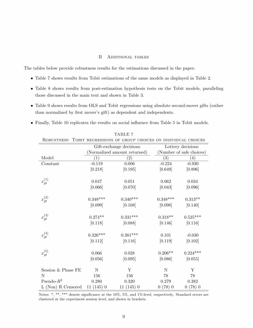
the model. 36
TABLE 2
OLS regressions of group choices on individual choices
Gift-exchange decisions Lottery decisions(Normalized amount returned) (Number of safe choices)
Session-Phase FE N Y N YN 156 156 78 78R2 0.771 0.811 0.505 0.618
Notes: *, **, *** denote significance at the 10%, 5%, and 1%-level, respectively. Standard errorsare clustered at the experiment session level, and shown in brackets.
In all models, the coefficient on the median member’s choice, β3, is positive and significant. In
gift-exchange decisions, also the second highest and the fourth highest individual choice contribute
to explaining the group choice, while the coefficients on the extreme individual choices β1 and β5 are
insignificant. In lottery choices, on the other hand, the member one position less risk-averse than the
median, as well as the most risk-averse member have a significant effect, besides the median member.
36Our hypotheses developed in Section 4 assume a linear structural model of how individual decisions are aggregatedto group decisions. Thus, reporting OLS estimates and running post-estimation hypotheses tests on their results (seeTable 3) is appropriate here. To test for robustness of our results, we ran the same models as Tobit specifications, andwith absolute gifts rather than normalized gifts, including the first mover’s offer as a control. The results are reported inthe Supplementary Appendix in Tables 7 and 9. In general, all our results and conclusions are robust to the specification.
16
When controlling for session-phase effects, the coefficient on x(5)gt stays significant, while the coefficient
on x(2)gt just misses the 10%-level with a p-value of p = 0.115.37
Our results do not support the hypothesis of a level shift – in both models (1) and (3) we do
not observe a significant constant α. Table 3 reports the results from post-estimation hypothesis tests
which directly test the competing hypotheses in Section 4 for the four OLS models reported in Table 2.
We reject both the weak and strong versions of the mean and the median hypotheses for all models:
neither are all five individual choices equally important, nor is only the median important and none
of the other individual decisions. Consistent with our finding that the constant is not significant in
models (1) and (3), we cannot reject the complementary hypothesis that the coefficients on individual
choices add up to 1 in any of our models. We also cannot reject the hypothesis that extreme choices
do not matter, except for model (4) on lottery decisions which includes session-phase fixed effects.
TABLE 3
Results from post-estimation hypothesis tests, p-values
ModelHypothesis (1) (2) (3) (4)
Weak mean 0.024** 0.051* 0.068* 0.061*Strong mean 0.032** <0.001*** 0.075* <0.001***Weak median 0.004*** 0.003*** 0.016** <0.001***Strong median 0.005*** 0.005*** <0.001*** <0.001***Extreme-irrelevance 0.339 0.953 0.131 <0.001***Convex combination 0.741 0.427 0.739 0.688
Note: *, **, *** denote significance at the 10%, 5%, and 1%-level, respectively.
5.c Order versus subject-specific effects
The results in the previous section establish that the median member, and certain other members have
significant influence on the group decision. However, they do not rule out that there are unobserved
individual characteristics, correlated with relative positions in groups, that determine how influential
different members are with respect to the group decision. Since each individual participates in 6 (3)
decisions in three different groups in our experiment, we can investigate this issue further, at the
individual level.
Below we compare three empirical models, in all of which the dependent variable is the absolute
difference between the group choice and an individual’s choice (∆gi). In the first model, we regress
this variable on a set of independents indicating the relative position of the individual in the given
group. In the second model, we aim to explain the same dependent variable purely by subject-specific
individual fixed effects. In the third model, we allow both the relative position within the group and
individual effects to influence the variable of interest. Formally, the models we investigate are:
37In Tobit versions of these analyses reported in Table 7 in the Supplementary Appendix, the coefficient of x(2)gt is
significant in model (4).
17
∆gi = α+ β1p(1)gi + β2p
(2)gi + β4p
(4)gi + β5p
(5)gi + εgi.
∆gi = α+ γi + εgi.
∆gi = α+ β1p(1)gi + β2p
(2)gi + β4p
(4)gi + β5p
(5)gi + γi + εgi.
In the above regression equations, γi with i ∈ {1, ..., N} represent subject fixed-effects, with the
constraint∑N
i=1 γi = 0. The variables p(k)gi indicate the (tie-weighted) relative position of individual i
in group g. If individual i’s position in the group is the unique kth lowest within the group, p(k)gi takes
the value of 1, while all p(k′)gi for k′ 6= k take the value 0. If individuals il1 , ..., ilm are tied at positions
k, ..., k+m then all p(k)gi for k ∈ {k, ..., k+m} take the value 1/|{k, ..., k+m}| and all other p
(k′)gi take
the value of 0. Thus, for example, if an individual i is tied with another group member at the lowest
value in the group, we would have p(1)gi = 0.5, p
(2)gi = 0.5, p
(3)gi = 0, p
(4)gi = 0, p
(5)gi = 0.
In our estimations, the indicator variable for the 3rd position (median) is omitted to avoid perfect
multicollinearity, in the presence of the constant term. Given this, the constant α represents the
average difference of the group choice from the median member. Coefficients β1, β2, β4, β5 represent
how much further away from the group choice the individual decisions of individuals at positions 1, 2,
4, and 5 are. To return to our example of individual i tied with another group member at positions 1
and 2, the post-estimation prediction of the difference between the group and the individual choice of
this subject according to the third model above would be the sum of constant, individual effect, and
weighted average of position-effects 1 and 2, ∆gi = α+ 0.5β1 + 0.5β2 + γi.
Table 4 summarises the results of our investigation, which are remarkably similar across our two
domains of decisions, gift-exchange and lottery choices. Models (1) and (4) show the estimates from
the first equation, which only includes order indicators. While being at positions 1 and 5 implies that
the group decision is significantly further away from the individual’s decision than from the median’s
decision, for positions 2 and 4 the difference is not significant or depends on the specification. In
models (2) and (4), using only subject fixed-effects as explanatory variables of the difference between
an individual’s choice and the choice of her group (the second equation above), we observe a drop in
explanatory power. Adding these subject fixed-effects to the base model with order indicators (the
third equation) increases the explanatory power only modestly, and has basically no effect on the size
and significance of the order coefficients.
In sum, the relative position of an individual choice within a group seems to be the most important
indicator of the individual’s impact on the group’s choice, and is particularly robust against controlling
for possible (unobserved) individual characteristics which might additionally influence an individual’s
effect on the group choice.
18
TABLE 4
OLS regressions of difference between individual and group choice
Notes: *, **, *** denote significance at the 10%, 5%, and 1%-level, respectively. Standard errorsare clustered at the experiment session level, and shown in brackets. Subject fixed-effects areconstrained in that their sum is equal to zero.
5.d Social influence
Our experimental design allows us to study the effect of group decisions on subsequent decisions of
the involved individuals. Subjects made two gift-exchange decisions and one lottery decision within
the same group, before being rematched to another group in the next of three phases. Thus, for
gift-exchange decisions, when looking at the first decision in a phase, the previous decision (in t− 1)
was made in a different group. For the second decision in a phase, however, the previous decision (in
t − 1) was made in the same group. The first two models presented in Table 5 regress the first and
second individual choice in a phase, respectively, on the subject’s own decisions in t− 1 as well as the
difference between the group’s choice and the own choice in t − 1. We find that the first individual
choice in a phase is correlated with the own previous decision, but not with the group choice in the
previous, different group. The second choice in a phase, however, is correlated both with the own
previous choice and with the difference between group decision and own decision in the same group in
t− 1 (such that when the group decision was more generous than the own decision in t− 1, the own
decision becomes more generous in t).
A similar analysis for lottery decisions in provided in the third model in Table 5. We find that the
current decision of an individual, besides being highly correlated with the own previous decision, is
19
TABLE 5
OLS regressions of current individual choices on choices made before in a differentgroup or the same group
Own decision in t–1 0.734*** 0.659*** 1.022***[0.064] [0.046] [0.027]
Diff to Group in t–1 0.061 0.176*** 0.393***[0.042] [0.045] [0.048]
N 260 390 260R2 0.478 0.338 0.679
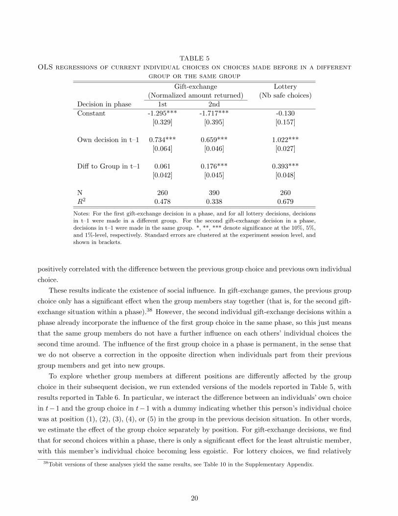
Notes: For the first gift-exchange decision in a phase, and for all lottery decisions, decisionsin t–1 were made in a different group. For the second gift-exchange decision in a phase,decisions in t–1 were made in the same group. *, **, *** denote significance at the 10%, 5%,and 1%-level, respectively. Standard errors are clustered at the experiment session level, andshown in brackets.
positively correlated with the difference between the previous group choice and previous own individual
choice.
These results indicate the existence of social influence. In gift-exchange games, the previous group
choice only has a significant effect when the group members stay together (that is, for the second gift-
exchange situation within a phase).38 However, the second individual gift-exchange decisions within a
phase already incorporate the influence of the first group choice in the same phase, so this just means
that the same group members do not have a further influence on each others’ individual choices the
second time around. The influence of the first group choice in a phase is permanent, in the sense that
we do not observe a correction in the opposite direction when individuals part from their previous
group members and get into new groups.
To explore whether group members at different positions are differently affected by the group
choice in their subsequent decision, we run extended versions of the models reported in Table 5, with
results reported in Table 6. In particular, we interact the difference between an individuals’ own choice
in t− 1 and the group choice in t− 1 with a dummy indicating whether this person’s individual choice
was at position (1), (2), (3), (4), or (5) in the group in the previous decision situation. In other words,
we estimate the effect of the group choice separately by position. For gift-exchange decisions, we find
that for second choices within a phase, there is only a significant effect for the least altruistic member,
with this member’s individual choice becoming less egoistic. For lottery choices, we find relatively
38Tobit versions of these analyses yield the same results, see Table 10 in the Supplementary Appendix.
20
TABLE 6
OLS regressions of current individual choices on choices made before, conditionalon previous position
Gift-exchange Lottery2nd decision in phase
(Normalized amount returned) (Nb safe choices)
Constant -1.939*** 0.012[0.406] [0.342]
Own decision in t–1 0.665*** 1.003***[0.04] [0.052]
Was (1) 0.296* 0.312**× Diff to Group in t–1 [0.146] [0.121]
Was (2) 0.063 0.16× Diff to Group in t–1 [0.194] [0.103]
Was (3) 0.189 0.07× Diff to Group in t–1 [0.115] [0.102]
Was (4) 0.069 -0.305× Diff to Group in t–1 [0.056] [0.185]
Was (5) 0.024 0.566***× Diff to Group in t–1 [0.102] [0.111]
N 260 260R2 0.338 0.679
Notes: *, **, *** denote significance at the 10%, 5%, and 1%-level, respectively. Standard errorsare clustered at the experiment session level, and shown in brackets.
strong significant effects for both the most risk-averse and the most risk-loving person, both of whom
adjust their subsequent lottery task decision towards the previous group choice.
These results suggest that deliberation not only suppresses extreme opinions in the current decision,
but that it also has a long-lasting effect by changing the opinions of extreme group members, bringing
them closer to the median.
6 Conclusion
This paper investigates how groups come to an agreement through deliberation, and which group
members have a significant influence on the group choice. We find that the member with the median
opinion has the greatest influence on the choice, but there are members in both direction from the
median who can also influence the choice. We observe that extreme opinions tend to be suppressed
in group decision making. We also find evidence that persuasion is part of deliberation, as individ-
ual opinions tend to move towards previous group decisions the individuals participated in. This
21
particularly holds for individuals with extreme opinions, implying that deliberation has a permanent
depolarizing effect in the population. This is consistent with the idea behind deliberative democracy,
in that deliberation, not merely voting, provides real authenticity to social choices.
References
Ambrus, A. and Lu, S.-E. (forthcoming), ‘A continuous-time model of multilateral bargaining’, Amer-
ican Economic Journal: Microeconomics .
Ambrus, A. and Pathak, P. (2012), ‘Cooperation over finite horizons: A theory and experiments’,
Journal of Public Economics 95, 500–512.
Arora, N. and Allenby, G. (1999), ‘Measuring the influence of individual preference structures in group
decision making’, Journal of Marketing Research 36, 476–487.
Baker, R. J., Laury, S. K. and Williams, A. W. (2008), ‘Comparing small-group and individual behavior
in lottery-choice experiments’, Southern Economic Journal 75, 367–382.
Banks, J. S. and Duggan, J. (2000), ‘A bargaining model of collective choice’, American Political
Science Review 94, 73–88.
Baron, D. P. and Ferejohn, J. A. (1989), ‘Bargaining in legislatures’, The American Political Science
Review 83(4), 1181–1206.
Bhaskar, V., Mailath, G. and Morris, S. (2013), ‘A foundation for markov equilibria in sequential
games with finite social memory’, Review of Economic Studies 80, 925–948.
Bhaskar, V. and Vega-Redondo, F. (2002), ‘Asynchronous choice and markov equilibria’, Journal of
Economic Theory 103(2), 334–350.
Blinder, A. and Morgan, J. (2005), ‘Are two heads better than one? an experimental analysis of group
versus individual decision making’, Journal of Money, Credit and Banking 37, 789–811.
Bornstein, G., Kugler, T. and Ziegelmeyer, A. (2004), ‘Individual and group decisions in the centipede
game: are groups more ”rational” players?’, Journal of Experimental Social Psychology 40, 599–605.
Bornstein, G. and Yaniv, I. (1998), ‘Individual and group behavior in the ultimatum game: Are groups
more ”rational” players?’, Experimental Economics 1(101-108).
Bower, J. (1965), ‘The role of conflict in economic decision-making groups: Some empirical results’,
Quarterly Journal of Economics 79, 263–277.
Brandts, J. and Charness, G. (2004), ‘Do labour market conditions affect gift exchange? some exper-
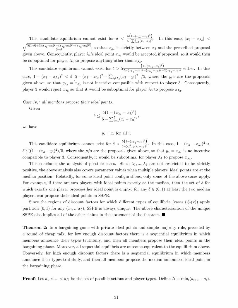
Setting the payoff of player 3 equal to v and setting y = xλ4 gives the next bound on δ:
5(1− (xλ4 − x3)2
)5−
∑5i=1(xi − x3)2
< δ ≤5(1− (xλ3 − x3)2
)5− (xλ1 − x3)2 − (xλ2 − x3)2 − 2(xλ3 − x3)2
.
Then, given the above inequality holds,
y3 = x3, yλk =
xλk if k ≤ 3
x3 −√
5(1−δ) + δ[(xλ1−x3)2 + (xλ2−x3)2 + (xλ3−x3)2]5− δ
if k=4, λ4<3
x3 +
√5(1−δ) + δ[(xλ1−x3)2 + (xλ2−x3)2 + (xλ3−x3)2]
5− δif k=4, λ4>3
30
This candidate equilibrium cannot exist for δ <5(1−(xλ4−x3)
2)
5−∑5i=1(xi−x3)2
. In this case, |x3 − xλ4 | <√5(1−δ)+δ[(xλ1−x3)
2+(xλ2−x3)2+(xλ3−x3)
2]
5−δ , so that xλ4 is strictly between x3 and the prescribed proposal
given above. Consequently, player λ4’s ideal point xλ4 would be accepted if proposed, so it would then
be suboptimal for player λ4 to propose anything other than xλ4 .
This candidate equilibrium cannot exist for δ > 5
(1−(xλ3−x3)
2)
5−(xλ1−x3)2−(xλ2−x3)
2−2(xλ3−x3)2 either. In this
case, 1 − (x3 − xλ3)2 < δ[5− (x3 − xλ3)2 −
∑i 6=λ3(x3 − yi)2
]/5, where the yi’s are the proposals
given above, so that yλ3 = xλ3 is not incentive compatible with respect to player 3. Consequently,
player 3 would reject xλ3 so that it would be suboptimal for player λ3 to propose xλ3 .
Case (v): all members propose their ideal points.
Given
δ ≤5(1− (xλ4 − x3)2
)5−
∑5i=1(xi − x3)2
,
we have
yi = xi for all i.
This candidate equilibrium cannot exist for δ >5(1−(xλ4−x3)
2)
5−∑5i=1(xi−x3)2
. In this case, 1 − (x3 − xλ4)2 <
δ∑(
1 − (x3 − yi)2)/5, where the yi’s are the proposals given above, so that y4 = xλ4 is no incentive
compatible to player 3. Consequently, it would be suboptimal for player λ4 to propose xλ4 .
This concludes the analysis of possible cases. Since λ1, ..., λ4 are not restricted to be strictly
positive, the above analysis also covers parameter values when multiple players’ ideal points are at the
median position. Relatedly, for some ideal point configurations, only some of the above cases apply.
For example, if there are two players with ideal points exactly at the median, then the set of δ for
which exactly one player proposes her ideal point is empty: for any δ ∈ (0, 1) at least the two median
players can propose their ideal points in SSPE.
Since the regions of discount factors for which different types of equilibria (cases (i)-(v)) apply
partition (0, 1) for any (x1, .., x5), SSPE is always unique. The above characterization of the unique
SSPE also implies all of the other claims in the statement of the theorem. �
Theorem 2: In a bargaining game with private ideal points and simple majority rule, preceded by
a round of cheap talk, for low enough discount factors there is a sequential equilibrium in which
members announce their types truthfully, and then all members propose their ideal points in the
bargaining phase. Moreover, all sequential equilibria are outcome-equivalent to the equilibrium above.
Conversely, for high enough discount factors there is a sequential equilibrium in which members
announce their types truthfully, and then all members propose the median announced ideal point in
the bargaining phase.
Proof: Let a1 < ... < aN be the set of possible actions and player types. Define ∆ ≡ mini(ai+1− ai).
31
Consider first the continuation game on the equilibrium path following the reporting stage. Note
that player 3’s continuation payoff at any stage, in case of no agreement, is δ, as according to the
candidate equilibrium profile all players propose x3 subsequently. Therefore δ ≥ 1 −∆2 implies that
player 3 rejects any proposal other than x3. Moreover, any proposal y < x3 gets rejected by players 4
and 5, and any proposal y > x3 gets rejected by players 1 and 2. Conversely, a proposal y = x3 gets
gets accepted by any player i, since it yields a payoff of 1− (xi−x3)2 > 0, which is strictly larger than
the continuation payoff δ(1− (xi−x3)2). This also implies that any player i strictly prefers proposing
x3 to any other proposal.
Now we consider the stage in which players report their valuations. Suppose a player with true
ideal point xi reports x′i 6= xi, and consider each of the possible cases: (a) misreporting leads other
players to believe the median ideal point is not xi, when in fact it is xi, (b) misreporting leads other
players to believe the median ideal point is not xj , when in fact it is xj 6= xi, (c) misreporting has no
effect on other players’ beliefs regarding the median ideal point.
For case (a), misreporting strictly decreases player i’s payoff because other players will no longer
propose player i’s ideal point if recognized in the first period. Therefore no matter how the game
proceeds thereafter, player i is strictly worse than if other players were to propose the true median of
xi in the first period.
For case (b), other players’ beliefs regarding the median ideal point can only be affected by player
i misreporting if xj is strictly between xi and x′i. Therefore, the perceived median, xj is further
from player i’s ideal point than the true median: |xj − xi| > |xj − xi|. Consequently, other players
(if recognized) propose xj , which gives player i a strictly worse payoff regardless of whether or not
the proposal is accepted than the payoff if other players propose (and accept) xj , as in the truthful
equilibrium.
For case (c), player i’s payoff is not affected by the deviation.
Therefore, player i cannot profit from misreporting in any of the three cases, and is strictly hurt by
misreporting in cases (a) and (b). Moreover, for any xi, player i’s ex-ante expectation of xi being the
true median ideal point is nonzero for a finite type space with independently distributed types. The
likelihood of strictly hurting oneself by misreporting is strictly positive for any xi. Thus, truth-telling
is the unique optimal action in the reporting stage. �
32
Supplementary Appendix to
Attila Ambrus, Ben Greiner, Parag A. Pathak:
”How individual preferences are aggregated in groups:
An experimental study”
(not for publication)
June 2014
A Theory
In this Supplementary Appendix we assume that ideal points are commonly known to be 0 ≤ x1 ≤... ≤ x5 ≤ 1, and that the agreement of all five players is required for a proposal to pass.
Convexity of Set of Acceptable Agreements
First we establish that the set of acceptable agreements, denoted by Y , in any SSPE is convex.
Given y1, . . . , y5, and conditional on all other players accepting, player i’s potential payoff from
accepting player j’s proposal yj is 1− (yj −xi)2, while the continuation value in case of no acceptance
is vi ≤ δ5 . The difference between the potential payoff from acceptance and the continuation value,
i.e. 1 − (yj − xi)2 − vi, is decreasing as |yj − xi| increases. Therefore, if 1 − (yj − xi)
2 − vi ≥ 0
and |yj′ − xi| < |yj − xi| both hold, we must have that 1 − (yj′ − xi)2 − vi(yj′) ≥ 0, implying that
yj′ — like yj — is in the acceptance region for player i. Thus, the set of proposals that player
i is willing to accept, denoted Yi, is convex. Furthermore, this set is the intersection of the unit
interval and a closed interval in R centered at xi: Yi = [0, 1] ∩ [xi − zj , xi + zj ], where zj > 0 is
implicitly defined above. Since the intersection of convex sets is convex, the set of mutually acceptable
agreements, Y ≡ Y1 ∩ . . . Y5, is also convex. Consequently, if xi ∈ Y and xi+k ∈ Y for k ≥ 1, then
xi+1 ∈ [xi, xi+k] ∈ Y . Therefore any player with an ideal point that is between the minimum and the
maximum ideal points of players who propose their ideal point in a given SSPE must also propose their
ideal point in that SSPE. This feature means we can limit our consideration to the cases covered below.
Case (i): all members propose their ideal points.
For one of the extreme members, n = {1, 5}, the incentive compatibility condition to lure all other
voters is
1− (x1 − x5)2 ≥ δ[5−5∑i=1
(xi − xn)2]/5,
which gives the upper bound on δ:
δ ≤ minn∈{1,5}
{5[1− (x5 − x1)2]
5−∑5
i=1(xi − xn)2
}.
Then, given the above inequality holds, yi = xi for all i.
1
This candidate equilibrium cannot exist for δ > minn∈{1,5}
{5[1−(x5−x1)2]
5−∑5i=1(xi−xn)2
}. In this case,
1 − (x3 − xm)2 < δ∑(
1 − (x3 − yi)2)/5, where the yi’s are the proposals given above and
m ≡ arg minn∈{1,5}
{5[1−(x5−x1)2]
5−∑5i=1(xi−xn)2
}, so that ym = xm is not incentive compatible to player 6 −m
(i.e. to the opposite extreme). Consequently, it would be suboptimal for player m to propose xm.
Case (ii): four consecutive members propose their ideal points.
Now, one – but not both – of the extreme members, n = {1, 5}, is willing to accept the other’s
ideal point. Thus, the corresponding range for δ is:
minn∈{1,5}
{5[1− (x5 − x1)2]
5−∑5
i=1(xi − xn)2
}≤ δ ≤ max
n∈{1,5}
{5[1− (x5 − x1)2]
5−∑5
i=1(xi − xn)2
}.
The incentive compatibility condition for n to accept the other extreme member’s offer is
v = δ[v + 4−4∑i=2
(xi − xn)2]/5
Define
γ ≡ arg maxn∈{1,5}
{5∑i=1
(xi − xn)2
}.
Provided δ is in the range specified above, letting the payoff function for γ equal to v and solving for
the other extreme member’s offer gives:
yk =
xk if : k ∈ {2, 3, 4, γ}
x1 +
√5(1−δ) + δ[(x2−x1)2 + (x3−x1)2 + (x4−x1)2]
5− δif k = 5, γ = 1
x5 −√
5(1−δ) + δ[(x2−x5)2 + (x3−x5)2 + (x4−x5)2]5− δ
if k = 1, γ = 5
This candidate equilibrium cannot exist for δ < minn∈{1,5}
{5[1−(x5−x1)2]
5−∑5i=1(xi−xn)2
}. In this case, |xγ −
x6−γ | <√
5(1−δ)+δ[(x2−x1)2+(x3−x1)2+(x4−x1)2]5−δ , so that x6−γ is strictly between xγ and the prescribed
proposal y6−γ given above. Consequently, player 6 − γ’s ideal point x6−γ is in the set of mutually
acceptable agreements (in particular, it is acceptable to the opposite extreme, γ), so that it is no
longer optimal for player 6− γ to propose anything other than x6−γ .
This candidate equilibrium cannot exist for δ > maxn∈{1,5}
{5[1−(x5−x1)2]
5−∑5i=1(xi−xn)2
}. In this case,
1− (x6−γ −xγ)2 < δ[5− (x6−γ − xγ)2 −
∑i 6=6−γ(yi − xγ)2
]/5, where the yi’s are the proposals given
above, so that yγ = xγ is not incentive compatible to player 6 − γ (i.e. to the opposite extreme).
Consequently, it would be suboptimal for player γ to propose xγ .
Case (iii): three consecutive members propose their ideal points.
2
In this case, neither extreme accepts the other’s ideal point, but accepts all other members’ ideal
points. The indifference conditions that determine the extreme members’ proposals are:
Session & Phase FE N Y N YN 156 156 78 78Pseudo-R2 0.280 0.320 0.279 0.382L (Non) R Censored 11 (145) 0 11 (145) 0 0 (78) 0 0 (78) 0
Notes: *, **, *** denote significance at the 10%, 5%, and 1%-level, respectively. Standard errors areclustered at the experiment session level, and shown in brackets.
9
TABLE 8
Robustness: Results from post-estimation hypothesis tests on Tobit modelsreported in Table 7, p-values
ModelHypothesis (1) (2) (3) (4)
Weak mean 0.003*** 0.013** 0.004*** 0.004***Strong mean 0.001*** <0.001*** 0.004*** <0.001***Weak median <0.001*** <0.001*** <0.001*** <0.001***Strong median <0.001*** <0.001*** <0.001*** <0.001***Extreme-irrelevance 0.356 0.764 0.050* <0.001***Convex combination 0.032** 0.025** 0.719 0.610
Note: *, **, *** denote significance at the 10%, 5%, and 1%-level, respectively.
TABLE 9
Robustness: OLS and Tobit regressions of group choices on individual choices ingift-exchange games, using absolute choices (amount returned out of 10)
First-mover’s gift 0.008 0.006 -0.017 -0.090[0.040] [0.070] [0.095] [0.111]
Session-Phase FE N Y N YN 156 156 156 156(Pseudo) R2 0.772 0.817 0.304 0.375L (Non) R Censored 71 (72) 13 71 (72) 13
Notes: *, **, *** denote significance at the 10%, 5%, and 1%-level, respectively.Standard errors are clustered at the experiment session level, and shown in brackets.
10
TABLE 10
Robustness: Tobit regressions of current individual choices on choices made beforein a different group or the same group
Own decision in t–1 0.768*** 0.687*** 1.022***[0.073] [0.051] [0.026]
Diff to Group in t–1 0.062 0.173*** 0.393***[0.044] [0.054] [0.048]
N 260 260 260Pseudo-R2 0.111 0.074 0.3501Left (Non) Right Censored 26 (233) 1 31 (358) 0 0 (260) 0
Note: See also notes to Table 5 in paper. *, **, *** denote significance at the 10%, 5%, and 1%-level,respectively. Standard errors are clustered at the experiment session level, and shown in brackets.