How Many Clusters? Which Clustering Method? Answers Via Model-Based Cluster Analysis 1 C. Fraley and A. E. Raftery Technical Report No. 329 Department of Statistics University of Washington Box 354322 Seattle, WA 98195-4322 USA 1 Funded by the Office of Naval Research under contracts N00014-96-1-0192 and N00014-96-1- 0330. Thanks go to Simon Byers for providing the NNclean denoising procedure.
Transcript
How Many Clusters? Which Clustering Method?Answers Via Model-Based Cluster Analysis 1
C. Fraley and A. E. Raftery
Technical Report No. 329
Department of StatisticsUniversity of Washington
Box 354322Seattle, WA 98195-4322 USA
1Funded by the Office of Naval Research under contracts N00014-96-1-0192 and N00014-96-1-0330. Thanks go to Simon Byers for providing the NNclean denoising procedure.
Abstract
We consider the problem of determining the structure of clustered data, without priorknowledge of the number of clusters or any other information about their composition. Dataare represented by a mixture model in which each component corresponds to a differentcluster. Models with varying geometric properties are obtained through Gaussian compo-nents with different parameterizations and cross-cluster constraints. Noise and outliers canbe modeled by adding a Poisson process component. Partitions are determined by the EM(expectation-maximization) algorithm for maximum likelihood, with initial values from ag-glomerative hierarchical clustering.
Models are compared using an approximation to the Bayes factor based on the BayesianInformation Criterion (BIC); unlike significance tests, this allows comparison of more thantwo models at the same time, and removes the restriction that the models compared benested. The problems of determining the number of clusters and the clustering methodare solved simultaneously by choosing the best model. Moreover, the EM result provides ameasure of uncertainty about the associated classification of each data point.
Examples are given, showing that this approach can give performance that is much betterthan standard procedures, which often fail to identify groups that are either overlapping orof varying sizes and shapes.
1 Parameterizations of Σk and their geometric interpretation. . . . . . . . . . . . . 42 Reciprocal condition estimates for model-based methods applied to the diabetes data. 12
List of Figures
1 Three-group classifications for diabetes data using various clustering methods. . . 22 EM for clustering via Gaussian mixtures. . . . . . . . . . . . . . . . . . . . . . 63 Clinical classification of the diabetes data. . . . . . . . . . . . . . . . . . . . . . 104 BIC and uncertainty for the diabetes data. . . . . . . . . . . . . . . . . . . . . 115 Model-based classification of a simulated minefield with noise. . . . . . . . . . . . 13
i
1 Introduction
We consider the problem of determining the intrinsic structure of clustered data when noinformation other than the observed values is available. This problem is known as clusteranalysis, and should be distinguished from the related problem of discriminant analysis, inwhich known groupings of some observations are used to categorize others and infer thestructure of the data as a whole.
Probability models have been proposed for quite some time as a basis for cluster analysis.In this approach, the data are viewed as coming from a mixture of probability distributions,each representing a different cluster. Recently, methods of this type have shown promise ina number of practical applications, including character recognition (Murtagh and Raftery[53]), tissue segmentation (Banfield and Raftery [7]), minefield and seismic fault detection(Dasgupta and Raftery [27]), identification of textile flaws from images (Campbell et al.[21]), and classification of astronomical data (Celeux and Govaert [24], Mukerjee et al. [51]).
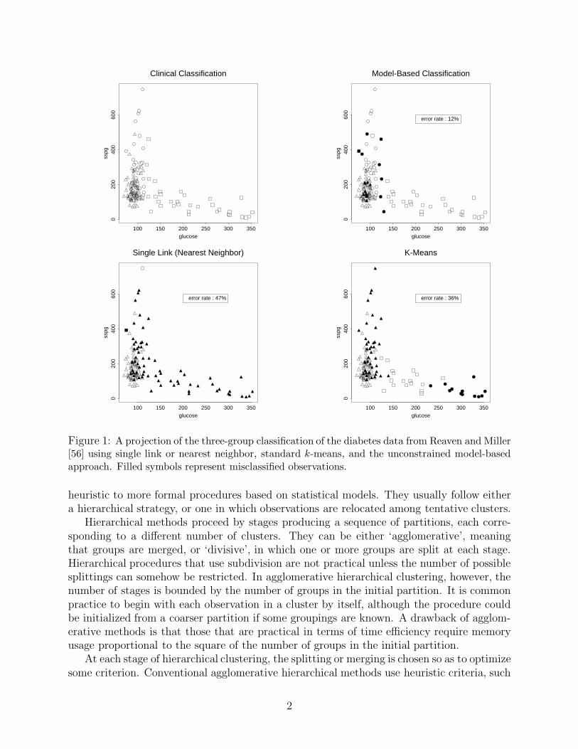
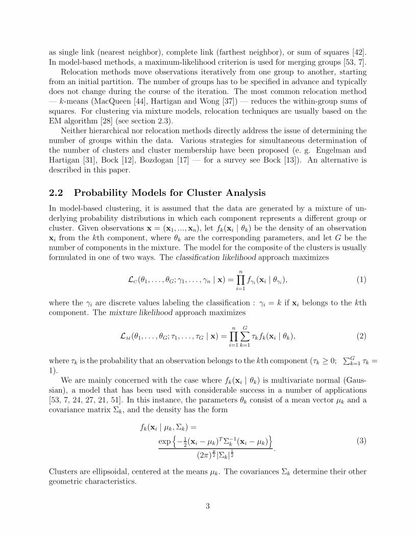
Bayes factors, approximated by the Bayesian Information Criterion (BIC), have beenapplied successfully to the problem of determining the number of components in a model[27], [51] and for deciding which among two or more partitions most closely matches thedata for a given model [21]. We describe a clustering methodology based on multivariatenormal mixtures in which the BIC is used for direct comparison of models that may differnot only in the number of components in the mixture, but also in the underlying densitiesof the various components. Partitions are determined (as in [27]) by a combination ofhierarchical clustering and the EM (expectation-maximization) algorithm (Dempster, Lairdand Rubin [28]) for maximum likelihood. This approach can give much better performancethan existing methods. Moreover, the EM result also provides a measure of uncertainty aboutthe resulting classification. Figure 1 shows an example in which model-based classificationis able to match the clinical classification of a biomedical data set much more closely thansingle-link (nearest-neighbor) or standard k-means, in the absence of any training data.
This paper is organized as follows. In Section 2, we give the necessary background inmultivariate cluster analysis, including discussions of probability models, the EM algorithmfor clustering and approximate Bayes factors. The basic model-based strategy and modi-fications for handling noise are described in Sections 2.5 and 2.6, respectively. A detailedanalysis of the multivariate data set shown in Figure 1 is given in Section 3.1, followed byan example from minefield detection in the presence of noise in Section 3.2. Information onavailable software for the various procedures used in this approach is given in Section 4. Afinal section summarizes and indicates extensions to the method.
2 Model-Based Cluster Analysis
2.1 Cluster Analysis Background
By cluster analysis we mean the partitioning of data into meaningful subgroups, when thenumber of subgroups and other information about their composition may be unknown; goodintroductions include Hartigan [36], Gordon [35], Murtagh [52], McLachlan and Basford [46],and Kaufman and Rousseeuw [42]. Clustering methods range from those that are largely
1
glucose
sspg
100 150 200 250 300 350
020
040
060
0
Clinical Classification
glucose
sspg
100 150 200 250 300 350
020
040
060
0
Model-Based Classification
error rate : 12%
glucose
sspg
100 150 200 250 300 350
020
040
060
0
Single Link (Nearest Neighbor)
error rate : 47%
glucose
sspg
100 150 200 250 300 350
020
040
060
0
error rate : 36%
K-Means
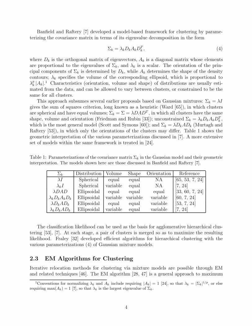
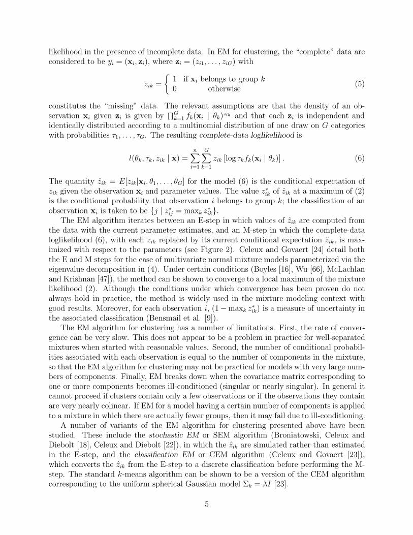
Figure 1: A projection of the three-group classification of the diabetes data from Reaven and Miller[56] using single link or nearest neighbor, standard k-means, and the unconstrained model-basedapproach. Filled symbols represent misclassified observations.
heuristic to more formal procedures based on statistical models. They usually follow eithera hierarchical strategy, or one in which observations are relocated among tentative clusters.
Hierarchical methods proceed by stages producing a sequence of partitions, each corre-sponding to a different number of clusters. They can be either ‘agglomerative’, meaningthat groups are merged, or ‘divisive’, in which one or more groups are split at each stage.Hierarchical procedures that use subdivision are not practical unless the number of possiblesplittings can somehow be restricted. In agglomerative hierarchical clustering, however, thenumber of stages is bounded by the number of groups in the initial partition. It is commonpractice to begin with each observation in a cluster by itself, although the procedure couldbe initialized from a coarser partition if some groupings are known. A drawback of agglom-erative methods is that those that are practical in terms of time efficiency require memoryusage proportional to the square of the number of groups in the initial partition.
At each stage of hierarchical clustering, the splitting or merging is chosen so as to optimizesome criterion. Conventional agglomerative hierarchical methods use heuristic criteria, such
2
as single link (nearest neighbor), complete link (farthest neighbor), or sum of squares [42].In model-based methods, a maximum-likelihood criterion is used for merging groups [53, 7].
Relocation methods move observations iteratively from one group to another, startingfrom an initial partition. The number of groups has to be specified in advance and typicallydoes not change during the course of the iteration. The most common relocation method— k-means (MacQueen [44], Hartigan and Wong [37]) — reduces the within-group sums ofsquares. For clustering via mixture models, relocation techniques are usually based on theEM algorithm [28] (see section 2.3).
Neither hierarchical nor relocation methods directly address the issue of determining thenumber of groups within the data. Various strategies for simultaneous determination ofthe number of clusters and cluster membership have been proposed (e. g. Engelman andHartigan [31], Bock [12], Bozdogan [17] — for a survey see Bock [13]). An alternative isdescribed in this paper.
2.2 Probability Models for Cluster Analysis
In model-based clustering, it is assumed that the data are generated by a mixture of un-derlying probability distributions in which each component represents a different group orcluster. Given observations x = (x1, ...,xn), let fk(xi | θk) be the density of an observationxi from the kth component, where θk are the corresponding parameters, and let G be thenumber of components in the mixture. The model for the composite of the clusters is usuallyformulated in one of two ways. The classification likelihood approach maximizes
LC(θ1, . . . , θG; γ1, . . . , γn | x) =n∏
i=1
fγi(xi | θγi), (1)
where the γi are discrete values labeling the classification : γi = k if xi belongs to the kthcomponent. The mixture likelihood approach maximizes
LM(θ1, . . . , θG; τ1, . . . , τG | x) =n∏
i=1
G∑k=1
τkfk(xi | θk), (2)
where τk is the probability that an observation belongs to the kth component (τk ≥ 0;∑G
k=1 τk =1).
We are mainly concerned with the case where fk(xi | θk) is multivariate normal (Gaus-sian), a model that has been used with considerable success in a number of applications[53, 7, 24, 27, 21, 51]. In this instance, the parameters θk consist of a mean vector µk and acovariance matrix Σk, and the density has the form
fk(xi | µk, Σk) =
exp{−1
2(xi − µk)T Σ−1
k (xi − µk)}
(2π)p2 |Σk|
12
.(3)
Clusters are ellipsoidal, centered at the means µk. The covariances Σk determine their othergeometric characteristics.
3
Banfield and Raftery [7] developed a model-based framework for clustering by parame-terizing the covariance matrix in terms of its eigenvalue decomposition in the form
Σk = λkDkAkDTk , (4)
where Dk is the orthogonal matrix of eigenvectors, Ak is a diagonal matrix whose elementsare proportional to the eigenvalues of Σk, and λk is a scalar. The orientation of the prin-cipal components of Σk is determined by Dk, while Ak determines the shape of the densitycontours; λk specifies the volume of the corresponding ellipsoid, which is proportional toλp
k |Ak|.1 Characteristics (orientation, volume and shape) of distributions are usually esti-mated from the data, and can be allowed to vary between clusters, or constrained to be thesame for all clusters.
This approach subsumes several earlier proposals based on Gaussian mixtures: Σk = λIgives the sum of squares criterion, long known as a heuristic (Ward [65]), in which clustersare spherical and have equal volumes; Σk = Σ = λDADT , in which all clusters have the sameshape, volume and orientation (Friedman and Rubin [33]); unconstrained Σk = λkDkAkDT
k ,which is the most general model (Scott and Symons [60]); and Σk = λDkADk (Murtagh andRaftery [53]), in which only the orientations of the clusters may differ. Table 1 shows thegeometric interpretation of the various parameterizations discussed in [7]. A more extensiveset of models within the same framework is treated in [24].
Table 1: Parameterizations of the covariance matrix Σk in the Gaussian model and their geometricinterpretation. The models shown here are those discussed in Banfield and Raftery [7].
Σk Distribution Volume Shape Orientation ReferenceλI Spherical equal equal NA [65, 53, 7, 24]λkI Spherical variable equal NA [7, 24]
The classification likelihood can be used as the basis for agglomerative hierarchical clus-tering [53], [7]. At each stage, a pair of clusters is merged so as to maximize the resultinglikelihood. Fraley [32] developed efficient algorithms for hierarchical clustering with thevarious parameterizations (4) of Gaussian mixture models.
2.3 EM Algorithms for Clustering
Iterative relocation methods for clustering via mixture models are possible through EMand related techniques [46]. The EM algorithm [28, 47] is a general approach to maximum
1Conventions for normalizing λk and Ak include requiring |Ak| = 1 [24], so that λk = |Σk|1/p, or elserequiring max(Ak) = 1 [7], so that λk is the largest eigenvalue of Σk.
4
likelihood in the presence of incomplete data. In EM for clustering, the “complete” data areconsidered to be yi = (xi, zi), where zi = (zi1, . . . , ziG) with
zik =
{1 if xi belongs to group k0 otherwise
(5)
constitutes the “missing” data. The relevant assumptions are that the density of an ob-servation xi given zi is given by
∏Gk=1 fk(xi | θk)zik and that each zi is independent and
identically distributed according to a multinomial distribution of one draw on G categorieswith probabilities τ1, . . . , τG. The resulting complete-data loglikelihood is
l(θk, τk, zik | x) =n∑
i=1
G∑k=1
zik [log τkfk(xi | θk)] . (6)
The quantity zik = E[zik|xi, θ1, . . . , θG] for the model (6) is the conditional expectation ofzik given the observation xi and parameter values. The value z∗ik of zik at a maximum of (2)is the conditional probability that observation i belongs to group k; the classification of anobservation xi is taken to be {j | z∗ij = maxk z∗
ik}.The EM algorithm iterates between an E-step in which values of zik are computed from
the data with the current parameter estimates, and an M-step in which the complete-dataloglikelihood (6), with each zik replaced by its current conditional expectation zik, is max-imized with respect to the parameters (see Figure 2). Celeux and Govaert [24] detail boththe E and M steps for the case of multivariate normal mixture models parameterized via theeigenvalue decomposition in (4). Under certain conditions (Boyles [16], Wu [66], McLachlanand Krishnan [47]), the method can be shown to converge to a local maximum of the mixturelikelihood (2). Although the conditions under which convergence has been proven do notalways hold in practice, the method is widely used in the mixture modeling context withgood results. Moreover, for each observation i, (1−maxk z∗
ik) is a measure of uncertainty inthe associated classification (Bensmail et al. [9]).
The EM algorithm for clustering has a number of limitations. First, the rate of conver-gence can be very slow. This does not appear to be a problem in practice for well-separatedmixtures when started with reasonable values. Second, the number of conditional probabil-ities associated with each observation is equal to the number of components in the mixture,so that the EM algorithm for clustering may not be practical for models with very large num-bers of components. Finally, EM breaks down when the covariance matrix corresponding toone or more components becomes ill-conditioned (singular or nearly singular). In general itcannot proceed if clusters contain only a few observations or if the observations they containare very nearly colinear. If EM for a model having a certain number of components is appliedto a mixture in which there are actually fewer groups, then it may fail due to ill-conditioning.
A number of variants of the EM algorithm for clustering presented above have beenstudied. These include the stochastic EM or SEM algorithm (Broniatowski, Celeux andDiebolt [18], Celeux and Diebolt [22]), in which the zik are simulated rather than estimatedin the E-step, and the classification EM or CEM algorithm (Celeux and Govaert [23]),which converts the zik from the E-step to a discrete classification before performing the M-step. The standard k-means algorithm can be shown to be a version of the CEM algorithmcorresponding to the uniform spherical Gaussian model Σk = λI [23].
5
initialize zik (this can be from a discrete classification (5))
repeat
M-step: maximize (6) given zik (fk as in (3)
nk ← ∑ni=1 zik
τk ← nk
n
µk ←∑n
i=1 zikxi
nk
Σk : depends on the model — see Celeux and Govaert [24]
E-step: compute zik given the parameter estimates from the M-step
zik ← τkfk(xi | µk, Σk)∑Gj=1 τjfj(xi | µj, Σj)
, where fk has the form (3).
until convergence criteria are satisfied
Figure 2: EM algorithm for clustering via Gaussian mixture models. The strategy described inthis paper initializes the iteration with indicator variables (5) corresponding to partitions fromhierarchical clustering, and terminates when the relative difference between successive values of themixture loglikelihood falls below a small threshold.
6
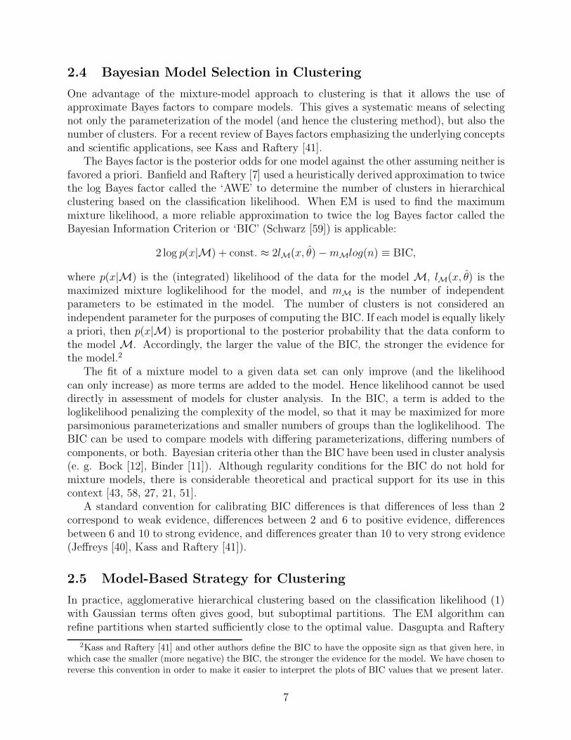
2.4 Bayesian Model Selection in Clustering
One advantage of the mixture-model approach to clustering is that it allows the use ofapproximate Bayes factors to compare models. This gives a systematic means of selectingnot only the parameterization of the model (and hence the clustering method), but also thenumber of clusters. For a recent review of Bayes factors emphasizing the underlying conceptsand scientific applications, see Kass and Raftery [41].
The Bayes factor is the posterior odds for one model against the other assuming neither isfavored a priori. Banfield and Raftery [7] used a heuristically derived approximation to twicethe log Bayes factor called the ‘AWE’ to determine the number of clusters in hierarchicalclustering based on the classification likelihood. When EM is used to find the maximummixture likelihood, a more reliable approximation to twice the log Bayes factor called theBayesian Information Criterion or ‘BIC’ (Schwarz [59]) is applicable:
where p(x|M) is the (integrated) likelihood of the data for the model M, lM(x, θ) is themaximized mixture loglikelihood for the model, and mM is the number of independentparameters to be estimated in the model. The number of clusters is not considered anindependent parameter for the purposes of computing the BIC. If each model is equally likelya priori, then p(x|M) is proportional to the posterior probability that the data conform tothe model M. Accordingly, the larger the value of the BIC, the stronger the evidence forthe model.2
The fit of a mixture model to a given data set can only improve (and the likelihoodcan only increase) as more terms are added to the model. Hence likelihood cannot be useddirectly in assessment of models for cluster analysis. In the BIC, a term is added to theloglikelihood penalizing the complexity of the model, so that it may be maximized for moreparsimonious parameterizations and smaller numbers of groups than the loglikelihood. TheBIC can be used to compare models with differing parameterizations, differing numbers ofcomponents, or both. Bayesian criteria other than the BIC have been used in cluster analysis(e. g. Bock [12], Binder [11]). Although regularity conditions for the BIC do not hold formixture models, there is considerable theoretical and practical support for its use in thiscontext [43, 58, 27, 21, 51].
A standard convention for calibrating BIC differences is that differences of less than 2correspond to weak evidence, differences between 2 and 6 to positive evidence, differencesbetween 6 and 10 to strong evidence, and differences greater than 10 to very strong evidence(Jeffreys [40], Kass and Raftery [41]).
2.5 Model-Based Strategy for Clustering
In practice, agglomerative hierarchical clustering based on the classification likelihood (1)with Gaussian terms often gives good, but suboptimal partitions. The EM algorithm canrefine partitions when started sufficiently close to the optimal value. Dasgupta and Raftery
2Kass and Raftery [41] and other authors define the BIC to have the opposite sign as that given here, inwhich case the smaller (more negative) the BIC, the stronger the evidence for the model. We have chosen toreverse this convention in order to make it easier to interpret the plots of BIC values that we present later.
7
[27] were able to obtain good results in a number of examples by using the partitions pro-duced by model-based hierarchical agglomeration as starting values for an EM algorithm forconstant-shape Gaussian models, together with the BIC to determine the number of clusters.Their approach forms the basis for a more general model-based strategy for clustering:
• Determine a maximum number of clusters to consider (M), and a set of candidateparameterizations of the Gaussian model to consider. In general M should be as smallas possible.
• Do agglomerative hierarchical clustering for the unconstrained Gaussian model,3 andobtain the corresponding classifications for up to M groups.
• Do EM for each parameterization and each number of clusters 2, . . . , M , startingwith the classification from hierarchical clustering.
• Compute the BIC for the one-cluster model for each parameterization, and for themixture likelihood with the optimal parameters from EM for 2, . . . , M clusters. Thisgives a matrix of BIC values corresponding to each possible combination of parame-terization and number of clusters.
• Plot the BIC values for each model. A decisive first local maximum indicates strongevidence for a model (parameterization + number of clusters).
It is important to avoid applying this procedure to a larger number of components thannecessary. One reason for this is to minimize computational effort; other reasons have beendiscussed in Section 2.3. A heuristic that works well in practice is to select the number ofclusters corresponding to the first decisive local maximum (if any) over all the parameteriza-tions considered. There may in some cases be local maxima giving larger values of BIC dueto ill-conditioning rather than a genuine indication of a better model (for further discussion,see section 3.1).
2.6 Modeling Noise and Outliers
Although the model-based strategy for cluster analysis as described in Section 2.5 is notdirectly applicable to noisy data, the model can be modified so that EM works well witha reasonably good initial identification of the noise and clusters. Noise is modeled as aconstant-rate Poisson process, resulting in the mixture likelihood
LM(θ1, . . . , θG; τ0, τ1, . . . , τG | x) =
∏ni=1
[τ0
V+
G∑k=1
τkfk(xi | θk)
],
(7)
where V is the hypervolume of the data region,∑G
k=0 τk = 1, and each fk(xi | θk) is mul-tivariate normal. An observation contributes 1/V if it belongs to the noise; otherwise itcontributes a Gaussian term.
3While there is a hierarchical clustering method corresponding to each parameterization of the Gaussianmodel, it appears to be sufficient in practice to use only the unconstrained model for initialization.
8
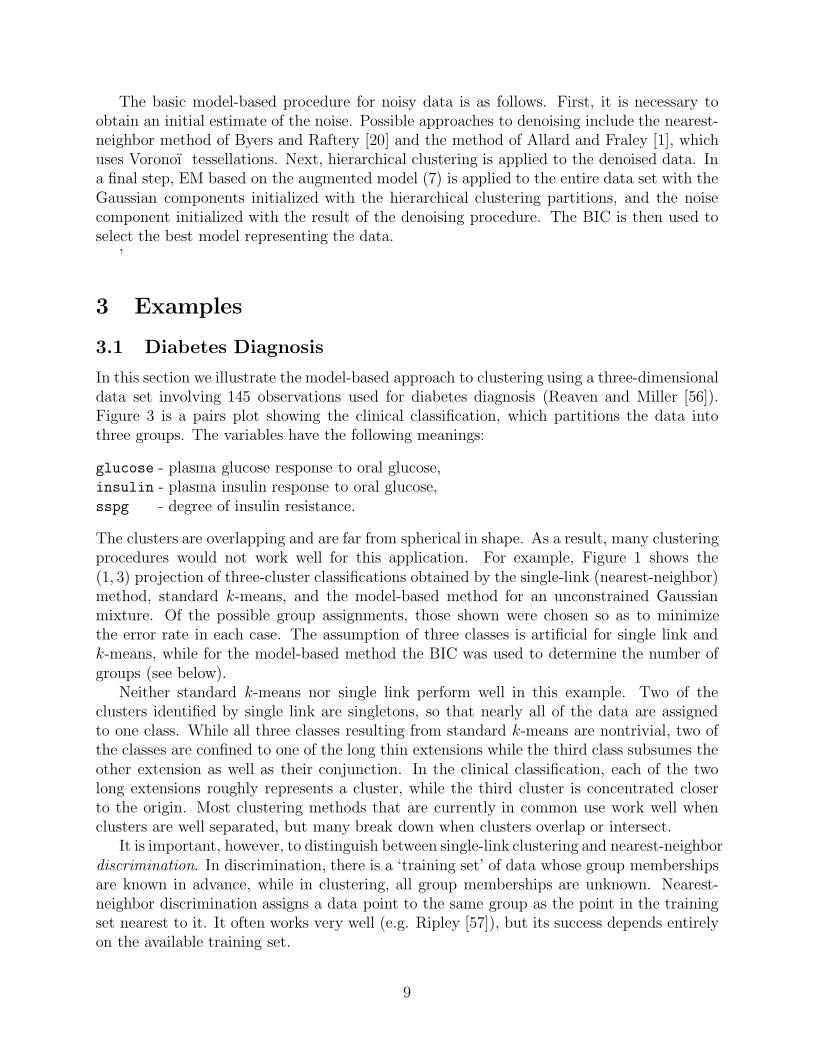
The basic model-based procedure for noisy data is as follows. First, it is necessary toobtain an initial estimate of the noise. Possible approaches to denoising include the nearest-neighbor method of Byers and Raftery [20] and the method of Allard and Fraley [1], whichuses Voronoı tessellations. Next, hierarchical clustering is applied to the denoised data. Ina final step, EM based on the augmented model (7) is applied to the entire data set with theGaussian components initialized with the hierarchical clustering partitions, and the noisecomponent initialized with the result of the denoising procedure. The BIC is then used toselect the best model representing the data.
’
3 Examples
3.1 Diabetes Diagnosis
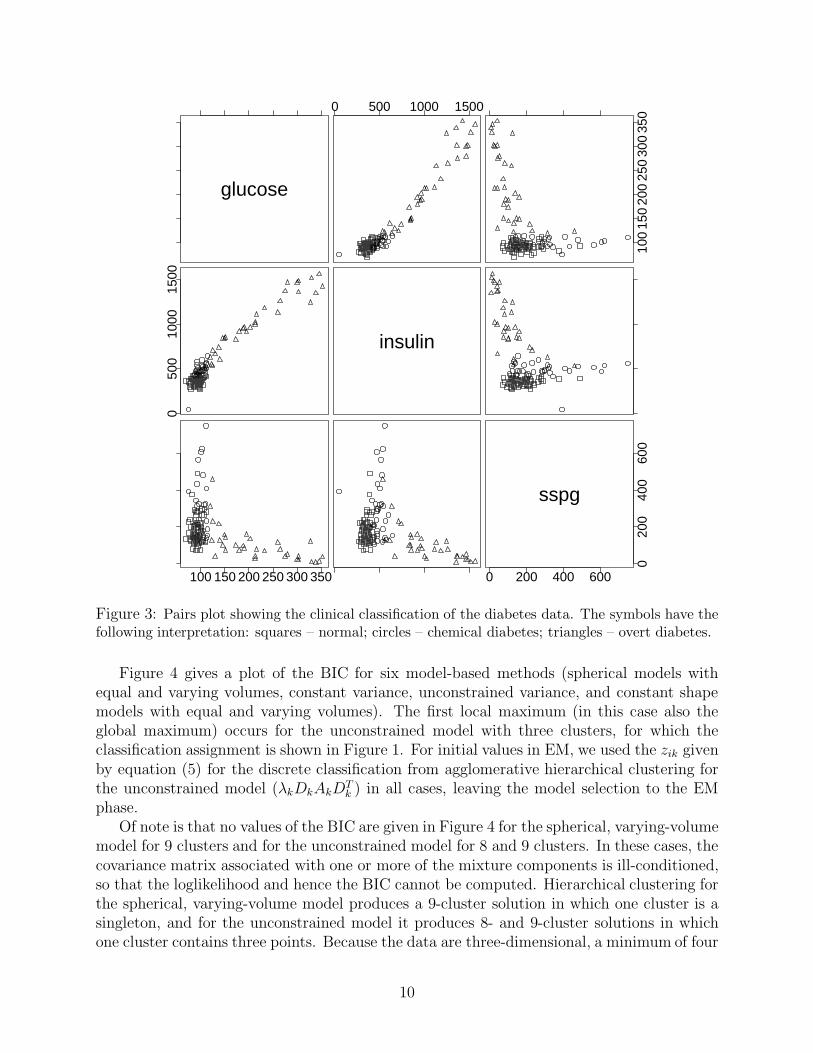
In this section we illustrate the model-based approach to clustering using a three-dimensionaldata set involving 145 observations used for diabetes diagnosis (Reaven and Miller [56]).Figure 3 is a pairs plot showing the clinical classification, which partitions the data intothree groups. The variables have the following meanings:
glucose - plasma glucose response to oral glucose,insulin - plasma insulin response to oral glucose,sspg - degree of insulin resistance.
The clusters are overlapping and are far from spherical in shape. As a result, many clusteringprocedures would not work well for this application. For example, Figure 1 shows the(1, 3) projection of three-cluster classifications obtained by the single-link (nearest-neighbor)method, standard k-means, and the model-based method for an unconstrained Gaussianmixture. Of the possible group assignments, those shown were chosen so as to minimizethe error rate in each case. The assumption of three classes is artificial for single link andk-means, while for the model-based method the BIC was used to determine the number ofgroups (see below).
Neither standard k-means nor single link perform well in this example. Two of theclusters identified by single link are singletons, so that nearly all of the data are assignedto one class. While all three classes resulting from standard k-means are nontrivial, two ofthe classes are confined to one of the long thin extensions while the third class subsumes theother extension as well as their conjunction. In the clinical classification, each of the twolong extensions roughly represents a cluster, while the third cluster is concentrated closerto the origin. Most clustering methods that are currently in common use work well whenclusters are well separated, but many break down when clusters overlap or intersect.
It is important, however, to distinguish between single-link clustering and nearest-neighbordiscrimination. In discrimination, there is a ‘training set’ of data whose group membershipsare known in advance, while in clustering, all group memberships are unknown. Nearest-neighbor discrimination assigns a data point to the same group as the point in the trainingset nearest to it. It often works very well (e.g. Ripley [57]), but its success depends entirelyon the available training set.
9
glucose
0 500 1000 1500
100
150
200
250
300
350
050
010
0015
00
insulin
100 150 200 250 300 350 0 200 400 600
020
040
060
0
sspg
Figure 3: Pairs plot showing the clinical classification of the diabetes data. The symbols have thefollowing interpretation: squares – normal; circles – chemical diabetes; triangles – overt diabetes.
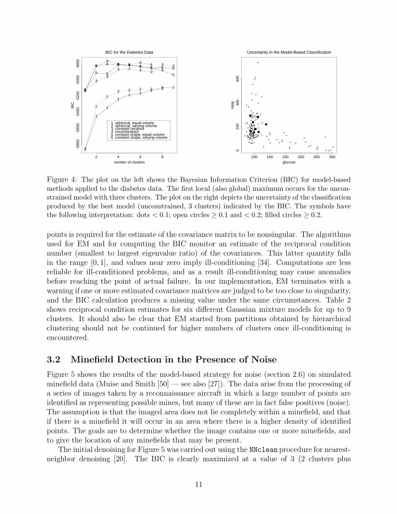
Figure 4 gives a plot of the BIC for six model-based methods (spherical models withequal and varying volumes, constant variance, unconstrained variance, and constant shapemodels with equal and varying volumes). The first local maximum (in this case also theglobal maximum) occurs for the unconstrained model with three clusters, for which theclassification assignment is shown in Figure 1. For initial values in EM, we used the zik givenby equation (5) for the discrete classification from agglomerative hierarchical clustering forthe unconstrained model (λkDkAkDT
k ) in all cases, leaving the model selection to the EMphase.
Of note is that no values of the BIC are given in Figure 4 for the spherical, varying-volumemodel for 9 clusters and for the unconstrained model for 8 and 9 clusters. In these cases, thecovariance matrix associated with one or more of the mixture components is ill-conditioned,so that the loglikelihood and hence the BIC cannot be computed. Hierarchical clustering forthe spherical, varying-volume model produces a 9-cluster solution in which one cluster is asingleton, and for the unconstrained model it produces 8- and 9-cluster solutions in whichone cluster contains three points. Because the data are three-dimensional, a minimum of four
Figure 4: The plot on the left shows the Bayesian Information Criterion (BIC) for model-basedmethods applied to the diabetes data. The first local (also global) maximum occurs for the uncon-strained model with three clusters. The plot on the right depicts the uncertainty of the classificationproduced by the best model (unconstrained, 3 clusters) indicated by the BIC. The symbols havethe following interpretation: dots < 0.1; open circles ≥ 0.1 and < 0.2; filled circles ≥ 0.2.
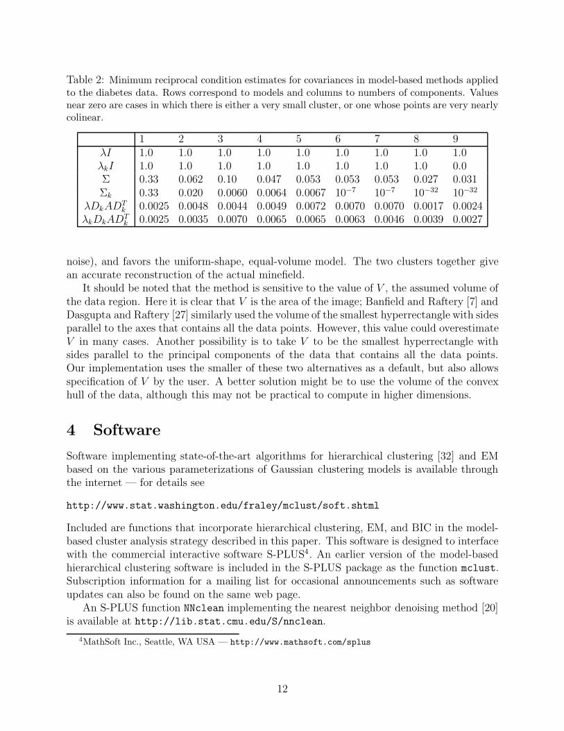
points is required for the estimate of the covariance matrix to be nonsingular. The algorithmsused for EM and for computing the BIC monitor an estimate of the reciprocal conditionnumber (smallest to largest eigenvalue ratio) of the covariances. This latter quantity fallsin the range [0, 1], and values near zero imply ill-conditioning [34]. Computations are lessreliable for ill-conditioned problems, and as a result ill-conditioning may cause anomaliesbefore reaching the point of actual failure. In our implementation, EM terminates with awarning if one or more estimated covariance matrices are judged to be too close to singularity,and the BIC calculation produces a missing value under the same circumstances. Table 2shows reciprocal condition estimates for six different Gaussian mixture models for up to 9clusters. It should also be clear that EM started from partitions obtained by hierarchicalclustering should not be continued for higher numbers of clusters once ill-conditioning isencountered.
3.2 Minefield Detection in the Presence of Noise
Figure 5 shows the results of the model-based strategy for noise (section 2.6) on simulatedminefield data (Muise and Smith [50] — see also [27]). The data arise from the processing ofa series of images taken by a reconnaissance aircraft in which a large number of points areidentified as representing possible mines, but many of these are in fact false positives (noise).The assumption is that the imaged area does not lie completely within a minefield, and thatif there is a minefield it will occur in an area where there is a higher density of identifiedpoints. The goals are to determine whether the image contains one or more minefields, andto give the location of any minefields that may be present.
The initial denoising for Figure 5 was carried out using the NNclean procedure for nearest-neighbor denoising [20]. The BIC is clearly maximized at a value of 3 (2 clusters plus
11
Table 2: Minimum reciprocal condition estimates for covariances in model-based methods appliedto the diabetes data. Rows correspond to models and columns to numbers of components. Valuesnear zero are cases in which there is either a very small cluster, or one whose points are very nearlycolinear.
noise), and favors the uniform-shape, equal-volume model. The two clusters together givean accurate reconstruction of the actual minefield.
It should be noted that the method is sensitive to the value of V , the assumed volume ofthe data region. Here it is clear that V is the area of the image; Banfield and Raftery [7] andDasgupta and Raftery [27] similarly used the volume of the smallest hyperrectangle with sidesparallel to the axes that contains all the data points. However, this value could overestimateV in many cases. Another possibility is to take V to be the smallest hyperrectangle withsides parallel to the principal components of the data that contains all the data points.Our implementation uses the smaller of these two alternatives as a default, but also allowsspecification of V by the user. A better solution might be to use the volume of the convexhull of the data, although this may not be practical to compute in higher dimensions.
4 Software
Software implementing state-of-the-art algorithms for hierarchical clustering [32] and EMbased on the various parameterizations of Gaussian clustering models is available throughthe internet — for details see
Included are functions that incorporate hierarchical clustering, EM, and BIC in the model-based cluster analysis strategy described in this paper. This software is designed to interfacewith the commercial interactive software S-PLUS4. An earlier version of the model-basedhierarchical clustering software is included in the S-PLUS package as the function mclust.Subscription information for a mailing list for occasional announcements such as softwareupdates can also be found on the same web page.
An S-PLUS function NNclean implementing the nearest neighbor denoising method [20]is available at http://lib.stat.cmu.edu/S/nnclean.
4MathSoft Inc., Seattle, WA USA — http://www.mathsoft.com/splus
Figure 5: Model-based classification of a simulated minefield with noise. Hierarchical clusteringwas first applied to data after 5 nearest neighbor denoising. EM was then applied to the full dataset with the noise term included in the model.
5 Discussion
We have described a clustering methodology based on multivariate normal mixture modelsand shown that it can give much better performance than existing methods. This approachuses model-based agglomerative hierarchical clustering to initialize the EM algorithm fora variety of models, and applies Bayesian model selection methods to determine the bestclustering method along with the number of clusters. The uncertainty associated with thefinal classification can be assessed through the conditional probabilities from EM.
This approach has some limitations, however. The first is that computational methodsfor hierarchical clustering have storage and time requirements that grow at a faster thanlinear rate relative to the size of the initial partition, so that they cannot be directly appliedto large data sets. One way around this is to determine the structure of some subset of thedata according to the strategy given here, and either use the resulting parameters as initialvalues for EM with all of the data, or else classify the remaining observations via supervised
13
classification or discriminant analysis [7]. Bensmail and Celeux [8] have developed a methodfor regularized discriminant analysis based on the full range of parameterizations of Gaussianmixtures (4). Alternatively, fast methods for determining an initial rough partition can beused to reduce computational requirements. Posse [55] suggested a method based on theminimum spanning tree for this purpose, and has shown that it works well in practice.
Second, although experience to date suggests that models based on the multivariatenormal distribution are sufficiently flexible to accommodate many practical situations, theunderlying assumption is that groups are concentrated locally about linear subspaces, sothat other models or methods may be more suitable in some instances. In Section 3.2,we obtained good results on noisy data by combining the model-based methodology witha separate denoising procedure. This example also suggests that nonlinear features can insome instances be well represented in the present framework as piecewise linear features,using several groups. There are alterative models in which classes are characterized bydifferent geometries such as linear manifolds (e. g. Bock [12], Diday [29], Spath [61]). Whenfeatures are strongly curvilinear, curves about which groups are centered can be modeled byusing principal curves (Hastie and Stuetzle [38]). Clustering about principal curves has beensuccessfully applied to automatic identification of ice-floe contours [5, 6], tracking of ice floes[3], and modeling ice-floe leads [4]. Initial estimation of ice-floe outlines is accomplished bymeans of mathematical morphology (e.g. [39]). Principal curve clustering in the presence ofnoise using BIC is discussed in Stanford and Raftery [62].
In situations where the BIC is not definitive, more computationally intensive Bayesiananalysis may provide a solution. Bensmail et al. [9] showed that exact Bayesian inference viaGibbs sampling, with calculations of Bayes factors using the Laplace-Metropolis estimator,works well in several real and simulated examples.
Approaches to clustering based on the classification likelihood (1) are also known asclassification maximum likelihood methods (e. g. McLachlan [45], Bryant and Williamson[19]) or fixed-classification methods (e. g. Bock [14, 13, 15]). There are alternatives to theclassification and mixture likelihoods given in section 2.2, such as the classification likelihoodof Symons [64]
The former is the complete data likelihood for the EM algorithm when the zik are restrictedto be indicator variables (5), while the later has the same form as the complete data likelihoodfor the EM algorithm, but includes the zik as parameters to be estimated. Fuzzy clusteringmethods (Bezdek [10]), which are not model-based, also provide degrees of membership forobservations.
The k-means algorithm has been applied not only to the classical sum-of-squares crite-rion but also to other model-based clustering criterion (e. g. Bock [12, 13, 15], Diday and
14
Govaert [30], Diday [29], Spath [61], Celeux and Govaert [24]). Other model-based clus-tering methodologies include Cheeseman and Stutz [25, 63], implemented in the AutoClass
software, and McLachlan et al. [46, 48, 54], implemented in the EMMIX (formerly MIXFIT)software. AutoClass handles both discrete data and continuous data, as well as data thathas both discrete and continuous variables. Both AutoClass for continuous data and EMMIX
rely on the EM algorithm for the multivariate normal distribution; EMMIX allows the choiceof either equal, unconstrained, or diagonal covariance matrices, while in Autoclass the co-variances are assumed to be diagonal. As in our approach, AutoClass uses approximateBayes factors to choose the number of clusters (see also Chickering and Heckerman [26]),although their approximation differs from the BIC. EMMIX determines the number of clustersby resampling, and has the option of modeling outliers by fitting mixtures of multivariatet-distributions (McLachlan and Peel [49]). In Autoclass, EM is initialized using randomstarting values, the number of trials being determined through specification of a limit on therunning time. Options for initializing EM in EMMIX include the most common heuristic hier-archical clustering methods, as well as k-means, whereas we use the model-based hierarchicalclustering solution as an initial value.
References
[1] D. Allard and C. Fraley. Nonparametric maximum likelihood estimation of features inspatial point processes using Voronoı tessellation. Journal of the American StatisticalAssociation, 92:1485–1493, December 1997.
[2] J. J. Anderson. Normal mixtures and the number of clusters problem. ComputationalStatistics Quarterly, 2:3–14, 1985.
[3] J. D. Banfield. Automated tracking of ice floes : A statistical approach. IEEE Trans-actions on Geoscience and Remote Sensing, 29(6):905–911, November 1991.
[4] J. D. Banfield. Skeletal modeling of ice leads. IEEE Transactions on Geoscience andRemote Sensing, 30(5):918–923, September 1992.
[5] J. D. Banfield and A. E. Raftery. Ice floe identification in satellite images using math-ematical morphology and clustering about principle curves. Journal of the AmericanStatistical Association, 87:7–16, 1992.
[6] J. D. Banfield and A. E. Raftery. Identifying ice floes in satellite images. Naval ResearchReviews, 43:2–18, 1992.
[7] J. D. Banfield and A. E. Raftery. Model-based Gaussian and non-Gaussian clustering.Biometrics, 49:803–821, 1993.
[8] H. Bensmail and G. Celeux. Regularized Gaussian discriminant analysis through eigen-value decomposition. Journal of the American Statistical Association, 91:1743–1748,December 1996.
15
[9] H. Bensmail, G. Celeux, A. E. Raftery, and C. P. Robert. Inference in model-basedcluster analysis. Statistics and Computing, 7:1–10, March 1997.
[10] J. C. Bezdek. Pattern Recognition with Fuzzy Objective Function Algorithms. Plenum,1981.
[11] D. A. Binder. Bayesian cluster analysis. Biometrika, 65:31–38, 1978.
[12] H. H. Bock. Automatische Klassifikation (Clusteranalyse). Vandenhoek & Ruprecht,1974.
[13] H. H. Bock. Probability models and hypotheis testing in partitioning cluster analysis.In P. Arabie, L. Hubert, and G. DeSorte, editors, Clustering and Classification, pages377–453. World Science Publishers, 1996.
[14] H. H. Bock. Probability models in partitional cluster analysis. Computational Statisticsand Data Analysis, 23:5–28, 1996.
[15] H. H. Bock. Probability models in partitional cluster analysis. In A. Ferligoj andA. Kramberger, editors, Developments in Data Analysis, pages 3–25. FDV, Metodoloskizvezki 12, Ljubljana, Slovenia, 1996.
[16] R. A. Boyles. On the convergence of the EM algorithm. Journal of the Royal StatisticalSociety, Series B, 45:47–50, 1983.
[17] H. Bozdogan. Choosing the number of component clusters in the mixture model usinga new informational complexity criterion of the inverse Fisher information matrix. InO. Opitz, B. Lausen, and R. Klar, editors, Information and Classification, pages 40–54.Springer-Verlag, 1993.
[18] M. Broniatowski, G. Celeux, and J. Diebolt. Reconnaissance de melanges de densitespar un algorithme d’apprentissage probabiliste. In E. Diday, M. Jambu, L. Lebart, J.-P.Pages, and R. Tomassone, editors, Data Analysis and Informatics, III, pages 359–373.Elsevier Science, 1984.
[19] P. Bryant and A. J. Williamson. Maximum likelihood and classification : a comparisonof three approaches. In W. Gaul and R. Schader, editors, Classification as a Tool ofResearch, pages 33–45. Elsevier Science, 1986.
[20] S. D. Byers and A. E. Raftery. Nearest neighbor clutter removal for estimating featuresin spatial point processes. Journal of the American Statistical Association, 93:577–584,June 1998.
[21] J. G. Campbell, C. Fraley, F. Murtagh, and A. E. Raftery. Linear flaw detection inwoven textiles using model-based clustering. Pattern Recognition Letters, 18:1539–1548,December 1997.
[22] G. Celeux and J. Diebolt. The SEM algorithm : A probabilistic teacher algorithmderived from the EM algorithm for the mixture problem. Computational StatisticsQuarterly, 2:73–82, 1985.
16
[23] G. Celeux and G. Govaert. A classification EM algorithm for clustering and two stochas-tic versions. Computational Statistics and Data Analysis, 14:315–332, 1992.
[24] G. Celeux and G. Govaert. Gaussian parsimonious clustering models. Pattern Recogni-tion, 28:781–793, 1995.
[25] P. Cheeseman and J. Stutz. Bayesian classification (AutoClass): Theory and results.In U. Fayyad, G. Piatesky-Shapiro, P. Smyth, and R. Uthurusamy, editors, Advancesin Knowledge Discovery and Data Mining, pages 153–180. AAAI Press, 1995.
[26] D. M. Chickering and D. Heckerman. Efficient approximations for the marginal likeli-hood of Bayesian networks with hidden variables. Machine Learning, 29:181–244, 1997.
[27] A. Dasgupta and A. E. Raftery. Detecting features in spatial point processes withclutter via model-based clustering. Journal of the American Statistical Association,93(441):294–302, March 1998.
[28] A. P. Dempster, N. M. Laird, and D. B. Rubin. Maximum likelihood for incompletedata via the EM algorithm. Journal of the Royal Statistical Society, Series B, 39:1–38,1977.
[29] E. Diday. Optimisation en classification automatique. INRIA (France), 1979.
[30] E. Diday and G. Govaert. Classification avec distances adaptives. Comptes RenduesAcad. Sci. Paris, serie A, 278:993, 1974.
[31] L. Engelman and J. A. Hartigan. Percentage points of a test for clusters. Journal ofthe American Statistical Association, 64:1647, 1969.
[32] C. Fraley. Algorithms for model-based Gaussian hierarchical clustering. SIAM Journalon Scientific Computing, 20(1):270–281, 1998.
[33] H. P. Friedman and J. Rubin. On some invariant criteria for grouping data. Journal ofthe American Statistical Association, 62:1159–1178, 1967.
[34] G. H. Golub and C. F. Van Loan. Matrix Computations. Johns Hopkins, 3rd edition,1996.
[35] A. D. Gordon. Classification: Methods for the Exploratory Analysis of MultivariateData. Chapman and Hall, 1981.
[36] J. A. Hartigan. Clustering Algorithms. Wiley, 1975.
[37] J. A. Hartigan and M. A. Wong. Algorithm AS 136 : A k-means clustering algorithm.Applied Statistics, 28:100–108, 1978.
[38] T. Hastie and W. Stuetzle. Principal curves. Journal of the American Statistical Asso-ciation, 84:502–516, 1989.
[39] H. J. A. M. Heijmans. Mathematical morphology: A modern approach in image pro-cessing based on algebra and geometry. SIAM Review, 37(1):1–36, March 1995.
17
[40] H. Jeffreys. Theory of Probability. Clarendon, 3rd edition, 1961.
[41] R. E. Kass and A. E. Raftery. Bayes factors. Journal of the American StatisticalAssociation, 90:773–795, 1995.
[42] L. Kaufman and P. J. Rousseeuw. Finding Groups in Data. Wiley, 1990.
[43] M. Leroux. Consistent estimation of a mixing distribution. The Annals of Statistics,20:1350–1360, 1992.
[44] J. MacQueen. Some methods for classification and analysis of multivariate observations.In L. M. Le Cam and J. Neyman, editors, Proceedings of the 5th Berkeley Symposiumon Mathematical Statistics and Probability, volume 1, pages 281–297. University of Cal-ifornia Press, 1967.
[45] G. McLachlan. The classification and mixture maximum likelihood approaches to clusteranalysis. In P. R. Krishnaiah and L. N. Kanal, editors, Handbook of Statistics, volume 2,pages 199–208. North-Holland, 1982.
[46] G. J. McLachlan and K. E. Basford. Mixture Models : Inference and Applications toClustering. Marcel Dekker, 1988.
[47] G. J. McLachlan and T. Krishnan. The EM Algorithm and Extensions. Wiley, 1997.
[48] G. J. McLachlan and D. Peel. Mixfit: An algorithm for automatic fitting and testingof normal mixtures. In Proceedings of the 14th International Conference on PatternRecognition, volume 1, pages 553–557. IEEE Computer Society, 1998.
[49] G. J. McLachlan and D. Peel. Robust cluster analysis via mixtures of multivariate t-distributions. In A. Amin, D. Dori, P. Pudil, and H. Freeman, editors, Lecture Notes inComputer Science, volume 1451, pages 658–666. Springer, 1998.
[50] R. Muise and C. Smith. Nonparametric minefield detection and localization. TechnicalReport CSS-TM-591-91, Coastal Systems Station, Panama City, Florida, 1991.
[51] S. Mukerjee, E. D. Feigelson, G. J. Babu, F. Murtagh, C. Fraley, and A. E. Raftery.Three types of gamma ray bursts. The Astrophysical Journal, 508:314–327, November1998.
[52] F. Murtagh. Multidimensional Clustering Algorithms, volume 4 of CompStat Lectures.Physica-Verlag, 1985.
[53] F. Murtagh and A. E. Raftery. Fitting straight lines to point patterns. Pattern Recog-nition, 17:479–483, 1984.
[54] D. Peel and G. J. McLachlan. User’s guide to EMMIX - version 1.0. University ofQueensland, Australia, 1998.
[55] C. Posse. Hierarchical model-based clustering for large data sets. Technical report,University of Minnesota, School of Statistics, 1998.
18
[56] G. M. Reaven and R. G. Miller. An attempt to define the nature of chemical diabetesusing a multidimensional analysis. Diabetologia, 16:17–24, 1979.
[57] B. D. Ripley. Neural networks and related methods for classification. Journal of theRoyal Statistical Society, Series B, 56:409–456, 1994.
[58] K. Roeder and L. Wasserman. Practical Bayesian density estimation using mixtures ofnormals. Journal of the American Statistical Association, 92:894–902, 1997.
[59] G. Schwarz. Estimating the dimension of a model. The Annals of Statistics, 6:461–464,1978.
[60] A. J. Scott and M. J. Symons. Clustering methods based on likelihood ratio criteria.Biometrics, 27:387–397, 1971.
[61] H. Spath. Cluster Dissection and Analysis: Theory, Fortran Programs, Examples. EllisHorwood, 1985.
[62] D. Stanford and A. E. Raftery. Principal curve clustering with noise. Technical Report317, University of Washington, Department of Statistics, February 1997.
[63] J. Stutz and P. Cheeseman. AutoClass - a Bayesian approach to classification. InJ. Skilling and S. Sibisi, editors, Maximum Entropy and Bayesian Methods, Cambridge1994. Kluwer, 1995.
[64] M. J. Symons. Clustering criteria and multivariate normal mixtures. Biometrics, 37:35–43, 1981.
[65] J. H. Ward. Hierarchical groupings to optimize an objective function. Journal of theAmerican Statistical Association, 58:234–244, 1963.
[66] C. F. J. Wu. On convergence properties of the EM algorithm. The Annals of Statistics,11:95–103, 1983.