How Many Stable EquilibriaWill a Large Complex System Have?

1

Yan V Fyodorov

Department of Mathematics

Project supported by the EPSRC grant EP/N009436/1

1Based on: YVF & B.A. Khoruzhenko Proc. Natl. Acad. Sci. USA 113,(25): 6827–6832 (2016);G. Ben Arous, YVF & B.A. Khoruzhenko, in progress

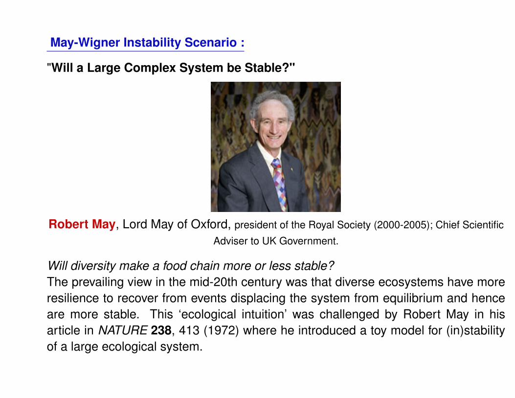
May-Wigner Instability Scenario :

"Will a Large Complex System be Stable?"

Robert May, Lord May of Oxford, president of the Royal Society (2000-2005); Chief Scientific

Adviser to UK Government.

Will diversity make a food chain more or less stable?The prevailing view in the mid-20th century was that diverse ecosystems have moreresilience to recover from events displacing the system from equilibrium and henceare more stable. This ‘ecological intuition’ was challenged by Robert May in hisarticle in NATURE 238, 413 (1972) where he introduced a toy model for (in)stabilityof a large ecological system.

May-Wigner Instability Scenario :

May suggested to consider a toy linear model for the dynamics of many interactingspecies represented by a state vector x ∈ RN :

x = −µx + Jx, µ > 0, x =

x1

. . .xN

Without interactions the part x = −µx describes a simple exponential relaxationof N uncoupled degrees of freedom xi with the same rate µ > 0 towards the stableequilibrium x = 0.

A complicated interaction between dynamics of different degrees of freedom ismimicked by a general real asymmetric N ×N random community matrix J withmean zero and prescribed variance α2 of all entries. As a typical eigenvalue of Jwith the largest real part grows as α

√N the equilibrium at x = 0 becomes unstable

as long as µ < µc = α√N .

This scenario is known in the literature as the "May-Wigner instability" and despiteits oversimplifying and schematic nature attracted very considerable attention inmathematical ecology and complex systems theory over the years.

Limitations of May-Wigner Instabilty Scenario:

• Typical evolution equations are generically nonlinear. The May’s analysis isessentially based on a linearization around a given equilibrium (set at x = 0) ,and hence tells us only about local asymptotic stability. It therefore does not allowto describe what may happen with the system when it does become unstable.

• The model has only limited bearing for dynamics of populations operating out-of-equilibrium. An instability does not necessarily imply lack of persistence:populations could coexist thanks to limit cycles or chaotic attractors, whichtypically originate from unstable equilibrium points. Interesting questions thenrelate to classification of equilibria by stability, studying the basins of attraction,and other features of global dynamics.

It is therefore desirable to have a generic nonlinear model which would be richenough to allow description of May-Wigner instability as a feature of its global phaseportrait, yet simple enough to allow analytical insights.

A Nonlinear Analogue of May-Wigner model:

We suggest a natural nonlinear extension of the May’s model to a system of Ncoupled nonlinear autonomous random ODE’s:

xi = −µxi + fi(x1, . . . , xN), i = 1, . . . , N

where couplings fi(x) represent components of an N−dimensional vector field andare chosen as a sum of a "gradient" and "solenoidal" contributions:

fi(x) = −∂V (x)∂xi

+ 1√N

∑Nj=1

∂Aij(x)

∂xj, i = 1, . . . , N

where we require the fields Aij(x) to be antisymmetric: Aij = −Aji. To make themodel as simple as possible and amenable to a detailed mathematical analysis wechoose the scalar potential V (x) and the fields Aij(x) to be independent mean zeroGaussian random fields, with additional assumptions of stationarity and isotropyw.r.t. the variables x = (x1, . . . , xN)T reflected in the covariance structure

E{V (x1)V (x2)} = v2ΓV(|x1 − x2|2

)E{Aij(x1)Anm(x2)} = a2ΓA

(|x1 − x2|2

)(δinδjm − δimδjn)

assuming certain smoothness of ΓV,A normalized such that Γ′′V (0) = Γ′′A(0) = 1.

Counting equilibria:

The standard analysis of autonomous ODE’s starts with finding equilibrium pointsand classifying them by stability properties.

Ideally, we would like to have the full statistical characterization of the total numberNtot(D) of all possible equilibria in a domain D of RN for the system of nonlinearautonomous random ODE’s :

xi = −µxi + fi(x1, . . . , xN), i = 1, . . . , N

and further of the numberNst(D) of stable equilibria attracting the dynamics in theirvicinity.

Control parameters of the model are:i) the ’May ratio’ of the relaxation rate to the characteristic value set by interaction:

m = µ/µc. µc =√N(a2 + v2)

ii) The ’non-potentiality’ parameter

τ = v2/(v2 + a2)

characterizing the ratio of variances of gradient and solenoidal components ofthe field such that τ = 0 corresponds to purely solenoidal, and τ = 1 to purelygradient descent dynamics.

Mean number of equilibria and the Elliptic Ensemble:

Using Kac-Rice approach we are able to count the mean values E{Ntot} andE{Nst} of all possible equilibria and of all stable equilibria. The first one turnsout to be given by the following integral:

E{Ntot} = 1mN

∫∞−∞ 〈|det (x−X)|〉X

e−Nt2

2 dt√2π/N

where x = m+t√τ , and the brackets 〈...〉X denote the averaging over the ensemble

of random real asymmetric matrix X known as the Gaussian Elliptic Ensemble:

P(X) = CN(τ)e− N

2(1−τ2)[TrXXT−τTrX2]

, τ ∈ [0, 1]

One can see that the real Ginibre ensemble corresponds to purely solenoidaldynamics with τ = 0, whereas GOE with τ = 1 corresponds to purely gradientdescent flow.Similarly, the mean number of stable equilibria is given by

E{Nst} = 1mN

∫∞−∞ 〈det (x−X)χx−X〉X

e−Nt2

2 dt√2π/N

where χA = 1 if all eigenvalues ofA have negative real parts, and χA = 0 otherwise.

A Nonlinear Analogue of May-Wigner Instability as Topology Detrivialization:

By relating 〈|det (x−X)|〉X to the mean density of real eigenvalues of the ellipticensemble and using the work by Forrester & Nagao ’07 one can find asymptotics ofE{Ntot} forN � 1. Such an analysis reveals a topology detrivialization transition,with the total number of equilibria abruptly changing from a single equilibrium forµ > µc =

√N(a2 + v2) to exponentially many equilibria as long as µ < µc.

Namely, for m = µµc

> 1 we have limN→∞E{Ntot} = 1 for any τ , whereas form = µ

µc< 1 and any 0 ≤ τ ≤ 1 we obtain instead

E{Ntot} ≈ K(τ,m) eNΣtot(m), Σtot(m) = m2−12 − lnm > 0

where the pre-exponential factor has the form

K(τ,m) =

√

2(1+τ)1−τ , for 0 ≤ τ < 1

4√

Nπ

∫√1−m2

0e−t

2u2dt for τ = 1− u2

N → 1

A qualitatively similar transition was reported recently in a model of randomly couplednonlinear ODE’s describing neural networks ( G. Wainrib & J. Touboul ’13).

Large Deviation Approach:

-2 -1.5 -1 -0.5 0 0.5 1 1.5 2

x

-2

-1.5

-1

-0.5

0

0.5

1

1.5

2

y

Elliptic rGinE(N=100, ==0.5)eigenvalues of 10 samples

x2/(1+=)2 +y2/(1-=)2=1

The asymptotic behaviour of

DN(x) = 〈det(x δij −Xij)χx−X〉

for large N � 1 can be extracted by exploiting the large deviation ideas, see e.g.Ben Arous & Zeitouni ’98. One finds

DN(x) ≈

{AN(x)eNΦ1(x), x > 1 + τ

BN(x)e−N2Iτ(x)+NΦ2(x), x < 1 + τ

whereΦ1(x) = 1

8τ

(x−√x2 − 4τ

)2+ ln

x+√x2−4τ2 ,

whereas the explicit form of the functions AN(x), BN(x), Iτ(x) and Φ2(x) is notactually needed for our purposes apart from the following facts:(i) Iτ(x) defined for all x ≤ 1 + τ has its minimum at x = 1 + τ and at that point itsvalue is zero: Iτ(1 + τ) = 0.

(ii) The functions Φ1(x) defined for x > 1 + τ and Φ2(x) defined for x < 1 + τsatisfy a continuity property limx→(1+τ)+0 Φ2(x) = limx→(1+τ)−0 Φ1(x) = τ

2 .

The mean number of stable equilibria in the topologically non-trivial phase:

Using the large deviation analysis, we were further able to show that the meannumber of stable equilibria satisfies asymptotically:

limN→∞1N lnE{Nst} = Σst(m; τ) = − lnm+ (m− 1)− (1−m)2

2τ

everywhere in the ’topologically non-trivial’ quadrant 0 < m < 1, 0 ≤ τ ≤ 1 of the(m, τ) plane. Moreover, there exists a curve τB(m) given explicitly by

τB(m) = − (1−m)2

2(1−m+lnm)

such that for a given m < 1 and τ < τB(m) the ’complexity function’ Σst(m; τ) isnegative, implying that the mean number of stable equilibria is exponentially small.This in turn implies that for such a regime the probability of having one or morestable equilibria is exponentially small, so in a typical realization of random ODE’sthere are simply no stable equilibria at all, i.e. Nst = 0. It is natural to name thistype of the phase portrait the ’absolute instability’ regime.

In contrast, for τ > τB(m) the complexity function Σst(m; τ) is positive so that stableequilibria are exponentially abundant. Still, for any m < 1, the stable equilibria areexponentially rare among all possible equilibria. One may call the associated type ofthe phase portrait as the ’relative instability’ regime.

Complexity of stable equilibria in the topologically non-trivial phase:

0 1 2

m

0

1

=Phase diagram in the (m,= )-plane

divergence free flow limit

absolute stability < N

tot > = <N

st> = 1

relative instability 0< '

st < '

tot

absolute instability '

st < 0, '

tot > 0

pure gradient flow limit

Σst < 0 below the line τB(m) implies that the probability of having one or more stable equilibria

is exponentially small though the total number of equilibria is exponentially big, hence ’absoluteinstabilty’ regime. Above the line stable equilibria are exponentially abundant but still are only

vanishing fraction among all equilibria.

Summary :

• As a generalization of the linear model by Robert May we suggest to consideran autonomous system of N nonlinear differential equations coupled by randomGaussian fields:

x = −µx + f(x)

• The problem of counting (on average) all possible equilibria, as well as of onlystable equilibria can be mapped onto the problem of evaluating the expected valueof the objects related to characteristic polynomial of random matrices from ’realelliptic ensemble’. The asymptotics of those objects forN � 1 can be efficientlystudied by either ’large deviation’ techniques, or, in particular instances, by relatingto real eigenvalues of elliptic matrices.

• The asymptotic analysis reveals that when the magnitude of randomcouplings increases with respect to the relaxation rate µ a single stableequilibrium is replaced by exponentially many equilibria via a sharp "topology(de)trivialization" transition. However, immediately after the transition none ofthose equilibria are stable, unless the dynamics is of purely gradient descenttype. Further increase in random couplings gives rise to exponentially many stableequilibria, unless the the dynamics is purely divergence-free, or ’solenoidal’.

Open questions:

• It is certainly important to further classify equilibria by ’index’ , that is to find howmany equilibria with a given number of unstable directions exist on average.

• Fluctuations in the number of equilibria of a given ’index’ is an interesting anddifficult open problem.

• Universality of the emerging picture for similar types of models (e.g. ’ non-relaxational spherical model dynamics’ (Cugliandolo et al. ’96), random neuralnetworks (Sompolinsky et al. ’88; Weinrib and Touboul ’13)

• Completely open are issues related to clarifying the global dynamical behaviourfor a generic non-potential random flow, existence & stability of limit cycles,emergence of chaotic dynamics and associated Lyapunov exponents, glassy andnon-equilibrium effects like ’aging’, etc.