How to model the interaction of charged Janus particles Reint Hieronimus 1,* , Simon Raschke 1 , and Andreas Heuer 1, ** 1 Westfälische Wilhelms-Universität Münster, Institut für physikalische Chemie, Corrensstraße 28/30, 48149 Münster, Germany Dated: 18 July 2016 We analyse the interaction of charged Janus particles including screening eects. The explicit interaction is mapped via a least square method on a variable number n of systematically generated tensors that reect the angular dependence of the potential. For n =2 we show that the interaction is equivalent to a model previously described by Erdmann, Kröger and Hess (EKH). Interestingly, this mapping is not able to capture the subtleties of the interaction for small screening lengths. Rather, a larger number of tensors has to be used. We nd that the characteristics of the Janus type interaction plays an important role for the aggregation behaviour. We obtained cluster structures up to the size of 13 particles for n =2 and 36 and screening lengths κ -1 =0.1 and 1.0 via Monte Carlo simulations. The inuence of the screening length is analysed and the structures are compared to results for an electrostatic-type potential and for multipole-expanded Derjaguin-Landau-Verwey-Overbeek (DLVO) theory. We nd that a dipole-like potential (EKH or dipole DLVO approximation) is not able to suciently reproduce the anisotropy eects of the potential. Instead, a higher order expansion has to be used to obtain clusters structures that are identical to experimental results for up to N =8 particles. The resulting minimum-energy clusters are compared to those of sticky hard sphere systems. Janus particles with a short-range screened interaction resemble sticky hard sphere clusters for all considered particle numbers, whereas for long-range screening even very small clusters are structurally dierent. 1. Introduction Janus particles are known for more than two decades, af- ter Veyssié and coworkers were able to prepare spheri- cal molecules with both a hydrophilic and a hydrophobic hemisphere [1] . Since then, they have been of large interest due to their anisotropic character, and today not only particles with hydrophilic-hydrophobic interaction [2,3] are synthetically accessible but also magnetic [4–6] or charged [7,8] particles. For a better understanding of the particle properties, eort has been put into theoretical investigations: the self-assembly behaviour and phase diagrams of hard spheres [9–11] and soft spheres [12,13] have been studied, for example, as well as the structure forma- tion on surfaces [14,15] and the interaction with surfaces [16] . Depending on the type of interaction, like patches either attract or repel each other. For an electrostatic interaction, which in this paper we are interested in, oppositely charged patches are attractive. Basic congurations are shown in Fig. 1. The ns conguration with the “north pole” of one particle pointing towards the “south pole” of another particle is the preferred conguration. By rotating the particles antiparallely towards their “equators” as in the ee conguration the interac- tion becomes gradually weaker. For the ee conguration the interaction is repulsive, and nally the nn conguration with touching “north poles” is the most repulsive. The potential of the not shown congurations ne or se is zero as here the interactions of the two “equators” cancel out each other. * Electronic mail: [email protected]** Electronic mail: [email protected]For the simulation of Janus particles in various systems a wide number of models reproducing their anisotropic prop- erties are known. The most straightforward approach is to model the particles as hard spheres and to use a square-well potential that is sensitive to the orientation of the patches, as introduced by Kern and Frenkel [17] . This potential can easily be implemented and is used quite often [10,11,18–24] . Also variants with distance-dependent potentials, such as Lennard-Jones or Yukawa, have been employed for the simulation of hard [25] and soft spheres [9,15,26–31] . For all these potentials an explicit expression, albeit slightly empirical, is given for the orientation dependence. ns ee nn ee Figure 1. Examples of congurations of two Janus particles in- cluding nomenclature. Depending on the type of interaction, like patches either attract or repel each other. 1 arXiv:1512.06053v2 [cond-mat.soft] 20 Jul 2016
Transcript
How to model the interaction ofcharged Janus particles
Reint Hieronimus1,*, Simon Raschke1, and Andreas Heuer1, **
We analyse the interaction of charged Janus particles including screening eUects. The explicit interaction is mapped viaa least square method on a variable number n of systematically generated tensors that reWect the angular dependenceof the potential. For n = 2 we show that the interaction is equivalent to a model previously described by Erdmann,Kröger and Hess (EKH). Interestingly, this mapping is not able to capture the subtleties of the interaction for smallscreening lengths. Rather, a larger number of tensors has to be used. We Vnd that the characteristics of the Janus typeinteraction plays an important role for the aggregation behaviour. We obtained cluster structures up to the size of 13particles for n = 2 and 36 and screening lengths κ−1 = 0.1 and 1.0 via Monte Carlo simulations. The inWuence ofthe screening length is analysed and the structures are compared to results for an electrostatic-type potential and formultipole-expanded Derjaguin-Landau-Verwey-Overbeek (DLVO) theory. We Vnd that a dipole-like potential (EKHor dipole DLVO approximation) is not able to suXciently reproduce the anisotropy eUects of the potential. Instead, ahigher order expansion has to be used to obtain clusters structures that are identical to experimental results for upto N = 8 particles. The resulting minimum-energy clusters are compared to those of sticky hard sphere systems.Janus particles with a short-range screened interaction resemble sticky hard sphere clusters for all considered particlenumbers, whereas for long-range screening even very small clusters are structurally diUerent.
1. Introduction
Janus particles are known for more than two decades, af-ter Veyssié and coworkers were able to prepare spheri-cal molecules with both a hydrophilic and a hydrophobichemisphere[1]. Since then, they have been of large interestdue to their anisotropic character, and today not only particleswith hydrophilic-hydrophobic interaction[2,3] are syntheticallyaccessible but also magnetic[4–6] or charged[7,8] particles. For abetter understanding of the particle properties, eUort has beenput into theoretical investigations: the self-assembly behaviourand phase diagrams of hard spheres[9–11] and soft spheres[12,13]
have been studied, for example, as well as the structure forma-tion on surfaces[14,15] and the interaction with surfaces[16].
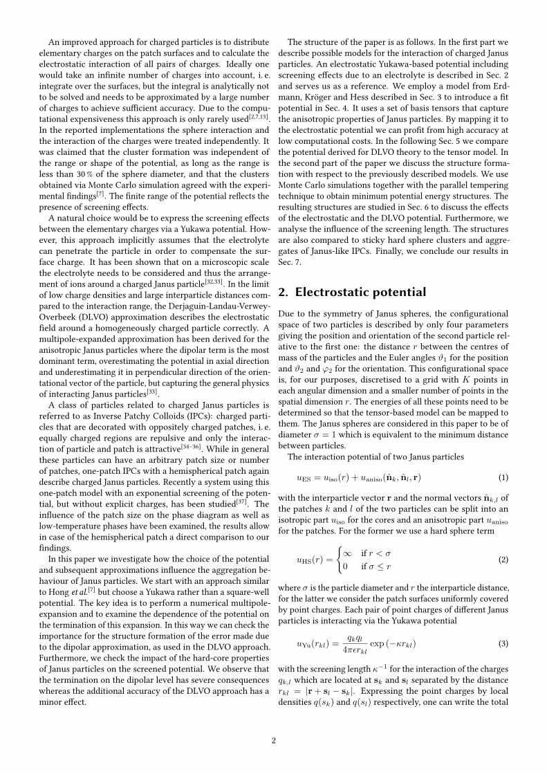
Depending on the type of interaction, like patches eitherattract or repel each other. For an electrostatic interaction,which in this paper we are interested in, oppositely chargedpatches are attractive. Basic conVgurations are shown in Fig. 1.The ns conVguration with the “north pole” of one particlepointing towards the “south pole” of another particle is thepreferred conVguration. By rotating the particles antiparallelytowards their “equators” as in the ee conVguration the interac-tion becomes gradually weaker. For the ee conVguration theinteraction is repulsive, and Vnally the nn conVguration withtouching “north poles” is the most repulsive. The potentialof the not shown conVgurations ne or se is zero as here theinteractions of the two “equators” cancel out each other.
For the simulation of Janus particles in various systems awide number of models reproducing their anisotropic prop-erties are known. The most straightforward approach is tomodel the particles as hard spheres and to use a square-wellpotential that is sensitive to the orientation of the patches, asintroduced by Kern and Frenkel[17]. This potential can easily beimplemented and is used quite often[10,11,18–24]. Also variantswith distance-dependent potentials, such as Lennard-Jones orYukawa, have been employed for the simulation of hard[25]
and soft spheres[9,15,26–31]. For all these potentials an explicitexpression, albeit slightly empirical, is given for the orientationdependence.
ns ee
nn ee
Figure 1. Examples of conVgurations of two Janus particles in-cluding nomenclature. Depending on the type of interaction, likepatches either attract or repel each other.
1
arX
iv:1
512.
0605
3v2
[co
nd-m
at.s
oft]
20
Jul 2
016
An improved approach for charged particles is to distributeelementary charges on the patch surfaces and to calculate theelectrostatic interaction of all pairs of charges. Ideally onewould take an inVnite number of charges into account, i. e.integrate over the surfaces, but the integral is analytically notto be solved and needs to be approximated by a large numberof charges to achieve suXcient accuracy. Due to the compu-tational expensiveness this approach is only rarely used[2,7,13].In the reported implementations the sphere interaction andthe interaction of the charges were treated independently. Itwas claimed that the cluster formation was independent ofthe range or shape of the potential, as long as the range isless than 30 % of the sphere diameter, and that the clustersobtained via Monte Carlo simulation agreed with the experi-mental Vndings[7]. The Vnite range of the potential reWects thepresence of screening eUects.
A natural choice would be to express the screening eUectsbetween the elementary charges via a Yukawa potential. How-ever, this approach implicitly assumes that the electrolytecan penetrate the particle in order to compensate the sur-face charge. It has been shown that on a microscopic scalethe electrolyte needs to be considered and thus the arrange-ment of ions around a charged Janus particle[32,33]. In the limitof low charge densities and large interparticle distances com-pared to the interaction range, the Derjaguin-Landau-Verwey-Overbeek (DLVO) approximation describes the electrostaticVeld around a homogeneously charged particle correctly. Amultipole-expanded approximation has been derived for theanisotropic Janus particles where the dipolar term is the mostdominant term, overestimating the potential in axial directionand underestimating it in perpendicular direction of the orien-tational vector of the particle, but capturing the general physicsof interacting Janus particles[33].
A class of particles related to charged Janus particles isreferred to as Inverse Patchy Colloids (IPCs): charged parti-cles that are decorated with oppositely charged patches, i. e.equally charged regions are repulsive and only the interac-tion of particle and patch is attractive[34–36]. While in generalthese particles can have an arbitrary patch size or numberof patches, one-patch IPCs with a hemispherical patch againdescribe charged Janus particles. Recently a system using thisone-patch model with an exponential screening of the poten-tial, but without explicit charges, has been studied[37]. TheinWuence of the patch size on the phase diagram as well aslow-temperature phases have been examined, the results allowin case of the hemispherical patch a direct comparison to ourVndings.
In this paper we investigate how the choice of the potentialand subsequent approximations inWuence the aggregation be-haviour of Janus particles. We start with an approach similarto Hong et al.[7] but choose a Yukawa rather than a square-wellpotential. The key idea is to perform a numerical multipole-expansion and to examine the dependence of the potential onthe termination of this expansion. In this way we can check theimportance for the structure formation of the error made dueto the dipolar approximation, as used in the DLVO approach.Furthermore, we check the impact of the hard-core propertiesof Janus particles on the screened potential. We observe thatthe termination on the dipolar level has severe consequenceswhereas the additional accuracy of the DLVO approach has aminor eUect.
The structure of the paper is as follows. In the Vrst part wedescribe possible models for the interaction of charged Janusparticles. An electrostatic Yukawa-based potential includingscreening eUects due to an electrolyte is described in Sec. 2and serves us as a reference. We employ a model from Erd-mann, Kröger and Hess described in Sec. 3 to introduce a Vtpotential in Sec. 4. It uses a set of basis tensors that capturethe anisotropic properties of Janus particles. By mapping it tothe electrostatic potential we can proVt from high accuracy atlow computational costs. In the following Sec. 5 we comparethe potential derived for DLVO theory to the tensor model. Inthe second part of the paper we discuss the structure forma-tion with respect to the previously described models. We useMonte Carlo simulations together with the parallel temperingtechnique to obtain minimum potential energy structures. Theresulting structures are studied in Sec. 6 to discuss the eUectsof the electrostatic and the DLVO potential. Furthermore, weanalyse the inWuence of the screening length. The structuresare also compared to sticky hard sphere clusters and aggre-gates of Janus-like IPCs. Finally, we conclude our results inSec. 7.
2. Electrostatic potential
Due to the symmetry of Janus spheres, the conVgurationalspace of two particles is described by only four parametersgiving the position and orientation of the second particle rel-ative to the Vrst one: the distance r between the centres ofmass of the particles and the Euler angles ϑ1 for the positionand ϑ2 and ϕ2 for the orientation. This conVgurational spaceis, for our purposes, discretised to a grid with K points ineach angular dimension and a smaller number of points in thespatial dimension r. The energies of all these points need to bedetermined so that the tensor-based model can be mapped tothem. The Janus spheres are considered in this paper to be ofdiameter σ = 1 which is equivalent to the minimum distancebetween particles.
The interaction potential of two Janus particles
uES = uiso(r) + uaniso(n̂k, n̂l, r) (1)
with the interparticle vector r and the normal vectors n̂k,l ofthe patches k and l of the two particles can be split into anisotropic part uiso for the cores and an anisotropic part uanisofor the patches. For the former we use a hard sphere term
uHS(r) =
{∞ if r < σ
0 if σ ≤ r(2)
where σ is the particle diameter and r the interparticle distance,for the latter we consider the patch surfaces uniformly coveredby point charges. Each pair of point charges of diUerent Janusparticles is interacting via the Yukawa potential
uYu(rkl) =qkql
4πεrklexp (−κrkl) (3)
with the screening length κ−1 for the interaction of the chargesqk,l which are located at sk and sl separated by the distancerkl = |r + sl − sk|. Expressing the point charges by localdensities q(sk) and q(sl) respectively, one can write the total
2
Table 1. Actual number of charges on the surface of a patch corre-sponding to the parameter L
Figure 2. Pearson correlation coeXcient of the electrostatic poten-tial uES for a variable value of L, displayed at the x-axis, and thevalue of L = 150. Here L is the parameter controlling the numberof charges per patch. Notice that the correlation is better for largerr as the values of the energy are lower due to the screening. Theenergies were determined with the screening length κ−1 = 0.1 andwithK = 10 subintervals in the angular dimensions.
interaction for every pair of patches after integration over bothpatch surfaces as
uYu(n̂k, n̂l, r) =
∫∫q(sk)q(sl)uYu(rkl) dsk dsl . (4)
The integration is carried out numerically using the trapezoidalrule and with a suXciently large number L of subintervals inϕ-direction, while in “longitudinal” ϑ-direction the numberis scaled by sinϑ to achieve a uniform coverage. The actualtotal number of charges per patch, as shown in Table 1, isapproximately given by 0.64L2.
As Janus particles have two hemispheres, summation overall four possible combinations of pairs of patches gives thetotal potential uES for each conVguration of two particles.
The accuracy of the resulting potential energy landscapedepends on the number K3 of grid points and the number0.64L2 of charges per patch. To Vnd a reasonable compromisebetween accuracy of the integration and computational time,we calculated the energies for L = 10, 20, 35, 50, 75, 100 andchecked via the Pearson coeXcient
ρ =
∑(u1 − 〈u1〉) (u2 − 〈u2〉)√∑
(u1 − 〈u1〉)2√∑
(u2 − 〈u2〉)2(5)
the correlation between these energies and those for L = 150.Here the sum is over all grid points. It shows that L = 35,i. e. 795 charges per patch, is already large enough to have abasically perfect determination of the integral (Fig. 2). For softJanus spheres with Coulomb interactions between the patches,a number of about 500 point charges per patch is found as theminimum value[13], corroborating our Vndings.
3. EKH potentialIn what follows, the orientation of two interacting Janus par-ticles are characterized by the two unit vectors n̂1,2 pointing
from the south pole to the north pole. The model describedby Erdmann, Kröger and Hess (EKH) makes use of sphericalharmonic tensors to capture the angular dependence of thepatch interaction[38]. These tensors need to fulVl the symmetryconditions
u(n̂1, n̂2, r) = −u(−n̂1, n̂2, r)
u(n̂1, n̂2, r) = −u(n̂1,−n̂2, r)
u(n̂1, n̂2, r) = u(n̂2, n̂1,−r)
(6)
in order to reWect the Janus geometry. The Vrst and secondcondition imply that the energy changes its sign if a particleis Wipped, the third means that the energy keeps its sign ifboth particles swap their positions and orientations. As a sideeUect, the orientational average vanishes for the anisotropicpart, i. e.
∫∫uaniso dn̂1 dn̂2 = 0. For Janus particles, second
rank tensors
ψ1 = (n̂1 · r̂)(n̂2 · r̂)− n̂1 · n̂2
3ψ2 = n̂1 · n̂2
(7)
are used by Erdmann, Kröger and Hess to deVne the scalaranisotropy function
ψEKH(n̂1, n̂2, r) = a1ψ1 + a2ψ2 (8)
via linear superposition. The tensors, coming from the S func-tions derived by Stone[39], are restricted to those compatiblewith conditions (6). The angular dependence of ψ1 correspondsto that of a dipole-dipole interaction and ψ2 acts as a pertur-bation that determines whether the equatorial or the polarconVgurations from Fig. 1 are preferred. An attractive interac-tion of like patches, as for hydrophilic-hydrophobic interaction,is indicated by positive signs of the coeXcients ai, while nega-tive signs indicate repulsive interaction as for charged patches.
As we want to model the previously described electrostaticpotential, we mapped the anisotropy function to the valuesof the electrostatic energies for every point in the discretisedconVgurational space while using the hard sphere potential forthe isotropic part. The distance dependence incorporated inthe Yukawa potential was Vtted with the function
a(r) =exp (−κr)
r3(a0 + a1r + a2r
2)
(9)
to the prefactors of the tensors. The Levenberg-Marquardtalgorithm was implemented to solve the nonlinear least-squareVts.
Within the limits of large screening lengths κ−1 and largeinterparticle distances r, the EKH potential proves to repro-duce the electrostatic potential well (Fig. 3a). However, withstronger screening the deviations get large especially for con-Vgurations where two patches are pointing directly towardseach other (Fig. 3b). These conVgurations have the largestenergy contributions and are therefore most important for theenergy of Janus clusters.
4. Mapping on a systematic tensorexpansion
To overcome the shortcomings of the EKH model a larger setof tensors is needed. Based on the S functions from Stone[39]
3
-0.09
-0.06
-0.03
0
0.03
0.06
0.09
-0.09 -0.06 -0.03 0 0.03 0.06 0.09
ufi
t
uES
uES = ufit
ψEKH (ρ = 0.9904)
(a) Screening length κ−1 = 1.0
-0.009
-0.006
-0.003
0
0.003
0.006
0.009
-0.009 -0.006 -0.003 0 0.003 0.006 0.009
ufi
t
uES
uES = ufit
ψEKH (ρ = 0.9435)
(b) Screening length κ−1 = 0.1
Figure 3. Comparison of electrostatic potential uES and the Vtpotential ufit using the EKH tensors. The energies were determinedfor Vxed interparticle distance r = 1.015 and with K = 10 andL = 50 integration subintervals. The yellow line visualizes an idealVt.
for a dipolar interaction, we get the tensors
ψa = n̂1 · r̂ψb = n̂2 · r̂ψc = n̂1 · n̂2
(10)
as a basis that is suXcient to describe the whole conVgurationalspace. The tensors ψa,b,c unambiguously determine the relatedenergy: if two conVgurations have identical basis tensors, theyalso have an identical energy. Employing the symmetry con-ditions (6), only certain combinations of ψa,b,c are allowed.By Wipping one of the particles the energy changes its sign,which means that in all combinations the normal vector n̂k,l
has to occur with an odd exponent. Furthermore, by swappingthe positions of the particles the sign of the energy needs tobe preserved, which means that the interparticle distance rijneeds to occur with an even exponent in all combinations. Thisyields
ψ =
B∑k
B∑j
B∑i
aijk (ψiaψ
jbψ
kc + ψj
aψibψ
kc ) (11)
as a systematic linear combination where j = i, i+2, i+4, . . .so that i + j is always even. Furthermore i + k has to beodd. The actual number of tensors in the Vnal Vt function isdetermined by the upper bound B of summation, as shown inTable 2.
The next step is to Vnd the smallest number of tensors thatis needed to reproduce the numerically determined electro-static potential uES with suXcient accuracy. Again we use
Table 2. Actual number of tensors used in the Vt function ufit
(a) Correlation between the electrostatic potential uES andthe Vt function ufit for upper bound B that determines theactual number of Vt tensors.
-0.009
-0.006
-0.003
0
0.003
0.006
0.009
-0.009 -0.006 -0.003 0 0.003 0.006 0.009
ufi
t
uES
uES = ufit
B = 3B = 5B = 7
(b) Comparison of electrostatic potential uES and the Vtpotential ufit using a number of tensors corresponding toB. The yellow line visualises an ideal Vt.
Figure 4. Determination of a reasonable number of tensors forthe Vt potential. The energies were determined with interparticledistance r = 1.015, screening length κ−1 = 0.1, and withK = 30and L = 50 integration subintervals.
the Pearson coeXcient and check the correlation between thevalues of the complete electrostatic and the Vtted potentialfor diUerent B (Fig. 4a). It is desirable to keep the number oftensors small for two reasons. First, it enables faster evalua-tion of the potential, which is of importance for time-eXcientsimulations. Second, the more parameters are available to theleast-square Vt algorithm the more numerical data is needed toavoid overVtting the potential. While this holds for the angulardimensions, the Vt of the distance-dependent function a(r)requires only a small number of points. We found that 36 ten-sors, corresponding to B = 5, yield good agreement betweenVt and electrostatic potential (Fig. 4). It is our reference to becompared to the potential with two tensors in the following.
We want to point out that for B = 1 the two tensors are
ψ1 = ψ110 = 2 (n̂1 · r̂)(n̂2 · r̂)
ψ2 = ψ001 = 2 n̂1 · n̂2
(12)
and that these are completely equivalent to the original EKHtensors (7) after straightforward deVnition of the prefactors.
4
Discussion of the potential
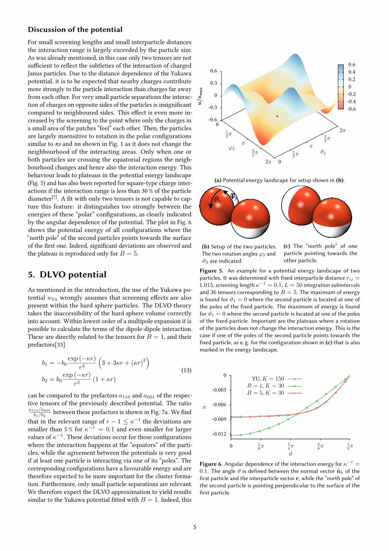
For small screening lengths and small interparticle distancesthe interaction range is largely exceeded by the particle size.As was already mentioned, in this case only two tensors are notsuXcient to reWect the subtleties of the interaction of chargedJanus particles. Due to the distance dependence of the Yukawapotential, it is to be expected that nearby charges contributemore strongly to the particle interaction than charges far awayfrom each other. For very small particle separations the interac-tion of charges on opposite sides of the particles is insigniVcantcompared to neighboured sides. This eUect is even more in-creased by the screening to the point where only the charges ina small area of the patches “feel” each other. Then, the particlesare largely insensitive to rotation in the polar conVgurationssimilar to ns and nn shown in Fig. 1 as it does not change theneighbourhood of the interacting areas. Only when one orboth particles are crossing the equatorial regions the neigh-bourhood changes and hence also the interaction energy. Thisbehaviour leads to plateaus in the potential energy landscape(Fig. 5) and has also been reported for square-type charge inter-actions if the interaction range is less than 30 % of the particlediameter[7]. A Vt with only two tensors is not capable to cap-ture this feature: it distinguishes too strongly between theenergies of these “polar” conVgurations, as clearly indicatedby the angular dependence of the potential. The plot in Fig. 6shows the potential energy of all conVgurations where the“north pole” of the second particles points towards the surfaceof the Vrst one. Indeed, signiVcant deviations are observed andthe plateau is reproduced only for B = 5.
5. DLVO potential
As mentioned in the introduction, the use of the Yukawa po-tential uYu wrongly assumes that screening eUects are alsopresent within the hard sphere particles. The DLVO theorytakes the inaccessibility of the hard sphere volume correctlyinto account. Within lowest order of a multipole expansion it ispossible to calculate the terms of the dipole-dipole interaction.These are directly related to the tensors for B = 1, and theirprefactors[33]
b1 = −b0exp (−κr)
r3
(3 + 3κr + (κr)
2)
b2 = b0exp (−κr)
r3(1 + κr)
(13)
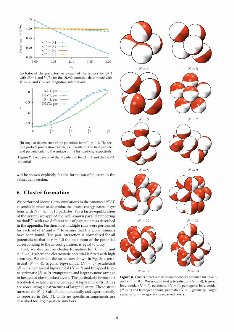
can be compared to the prefactors a110 and a001 of the respec-tive tensors of the previously described potential. The ratioa110/a001
b1/b2between these prefactors is shown in Fig. 7a. We Vnd
that in the relevant range of r − 1 ≤ κ−1 the deviations aresmaller than 5 % for κ−1 = 0.1 and even smaller for largervalues of κ−1. These deviations occur for those conVgurationswhere the interaction happens at the “equators” of the parti-cles, while the agreement between the potentials is very goodif at least one particle is interacting via one of its “poles”. Thecorresponding conVgurations have a favourable energy and aretherefore expected to be more important for the cluster forma-tion. Furthermore, only small particle separations are relevant.We therefore expect the DLVO approximation to yield resultssimilar to the Yukawa potential Vtted with B = 1. Indeed, this
012π
π32π
2π 0
12π
π
32π
2π
-0.6
-0.3
0
0.3
0.6
u/u
max
ϕ2ϑ2
u/u
max 0
-0.6-0.4-0.2
0.20.40.6
(a) Potential energy landscape for setup shown in (b).
(b) Setup of the two particles.The two rotation angles ϕ2 andϑ2 are indicated.
(c) The “north pole” of oneparticle pointing towards theother particle.
Figure 5. An example for a potential energy landscape of twoparticles. It was determined with Vxed interparticle distance rij =1.015, screening length κ−1 = 0.1, L = 50 integration subintervalsand 36 tensors corresponding to B = 5. The maximum of energyis found for ϑ1 = 0 where the second particle is located at one ofthe poles of the Vxed particle. The maximum of energy is foundfor ϑ1 = 0 where the second particle is located at one of the polesof the Vxed particle. Important are the plateaus where a rotationof the particles does not change the interaction energy. This is thecase if one of the poles of the second particle points towards theVxed particle, as e. g. for the conVguration shown in (c) that is alsomarked in the energy landscape.
0
-0.012
-0.009
-0.006
-0.003
0 18π 1
4π 3
8π 1
2π
u
ϑ
YU, K = 150B = 1, K = 30B = 5, K = 30
Figure 6. Angular dependence of the interaction energy for κ−1 =0.1. The angle ϑ is deVned between the normal vector n̂k of theVrst particle and the interparticle vector r, while the “north pole” ofthe second particle is pointing perpendicular to the surface of theVrst particle.
5
0.85
0.90
0.95
1.00
1.05
1.00 1.05 1.10 1.15 1.20
(a110/a
001)/(b
1/b
2)
rij
κ−1 = 0.1κ−1 = 0.2κ−1 = 0.3κ−1 = 1.0
(a) Ratio of the prefactors a110/a001 of the tensors for EKHwith B = 1 and b1/b2 for the DLVO potential, determined withK = 30 and L = 50 integration subintervals.
-0.9
-0.6
-0.3
0.0
0 18π 1
4π 3
8π 1
2π
u
ϑ
B = 1, parDLVO, parB = 1, per
DLVO, per
(b) Angular dependence of the potentials for κ−1 = 0.1. The sec-ond particle points downwards, i. e. parallel to the Vrst particle,and perpendicular to the surface of the Vrst particle, respectively.
Figure 7. Comparison of the Vt potential for B = 1 and the DLVOpotential.
will be shown explicitly for the formation of clusters in thesubsequent section.
6. Cluster formation
We performed Monte Carlo simulations in the canonical NV Tensemble in order to determine the lowest-energy states of sys-tems with N = 4, . . . , 13 particles. For a faster equilibrationof the system we applied the well-known parallel temperingmethod[40] with two diUerent sets of parameters as describedin the appendix. Furthermore, multiple runs were performedfor each set of B and κ−1 to ensure that the global minimahave been found. The pair interaction is normalized for allpotentials so that at r = 1.0 the maximum of the potential,corresponding to the ns conVguration, is equal to unity.
First, we discuss the cluster formation for B = 5 andκ−1 = 0.1 where the electrostatic potential is Vtted with highaccuracy. We obtain the structures shown in Fig. 8: a tetra-hedral (N = 4), trigonal bipyramidal (N = 5), octahedral(N = 6), pentagonal bipyramidal (N = 7) and tricapped trigo-nal prismatic (N = 9) arrangement, and larger systems arrangein hexagonal close-packed layers. The particularly favourabletetrahedral, octahedral and pentagonal bipyramidal structuresare reoccurring substructures of larger clusters. These struc-tures are forN ≤ 8 also found numerically and experimentallyas reported in Ref. [7], while no speciVc arrangements aredescribed for larger particle numbers.
N = 4 N = 5
N = 6 N = 7
N = 8 N = 9
N = 10 N = 11
N = 12 N = 13
Figure 8. Cluster structures with lowest energy obtained forB = 5and κ−1 = 0.1. We notably Vnd a tetrahedral (N = 4), trigonalbipyramidal (N = 5), octahedral (N = 6), pentagonal bipyramidal(N = 7) and tricapped trigonal prismatic (N = 9) geometry. Largersystems form hexagonal close-packed layers.
6
N = 4 N = 5
N = 6 N = 7
N = 8 N = 9
N = 10 N = 11
N = 12 N = 13
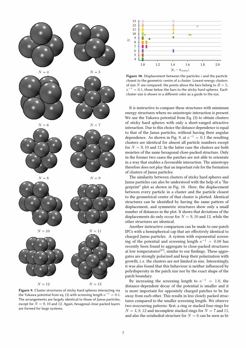
Figure 9. Cluster structures of sticky hard spheres interacting viathe Yukawa potential from eq. (3) with screening length κ−1 = 0.1.The arrangements are largely identical to those of Janus particles,except for N = 9, 10 and 12. Again, hexagonal close-packed layersare formed for large systems.
456789
10111213
1.0 1.2 1.4 1.6 1.8 2.0
N
|ri − rcenter|Figure 10. Displacement between the particles i and the particleclosest to the geometric centre of a cluster. Lowest-energy clustersof size N are compared: the points above the bars belong to B = 5,κ−1 = 0.1, those below the bars to the sticky hard spheres. Eachcluster size is shown in a diUerent color as a guide to the eye.
It is instructive to compare these structures with minimumenergy structures where no anisotropic interaction is present.We use the Yukawa potential from Eq. (3) to obtain clustersof sticky hard spheres with only a short-ranged attractiveinteraction. Due to this choice the distance dependence is equalto that of the Janus particles, without having their angulardependence. As shown in Fig. 9, at κ−1 = 0.1 the resultingclusters are identical for almost all particle numbers exceptfor N = 9, 10 and 12. In the latter case the clusters are bothmoieties of the same hexagonal close-packed structure. Onlyin the former two cases the patches are not able to orientatein a way that enables a favourable interaction. The anisotropytherefore does not play that an important role for the formationof clusters of Janus particles.
The similarity between clusters of sticky hard spheres andJanus particles can also be understood with the help of a “Vn-gerprint” plot as shown in Fig. 10. Here, the displacementbetween every particle in a cluster and the particle closestto the geometrical centre of that cluster is plotted. Identicalstructures can be identiVed by having the same pattern ofdisplacement, and symmetric structures show only a smallnumber of distances in the plot. It shows that deviations of thedisplacements do only occur for N = 9, 10 and 12, while theother structures are identical.
Another instructive comparison can be made to one-patchIPCs with a hemispherical cap that are eUectively identical tocharged Janus particles. A system with exponential screen-ing of the potential and screening length κ−1 = 0.08 hasrecently been found to aggregate to close-packed structuresat low temperatures[37], similar to our Vndings. These aggre-gates are strongly polarized and keep their polarization withgrowth, i. e. the clusters are not limited in size. Interestingly,it was also found that this behaviour is neither inWuenced bypolydispersity in the patch size nor by the exact shape of thepatch boundary.
By increasing the screening length to κ−1 = 1.0, thedistance-dependent decay of the potential is smaller and itis more important for oppositely charged patches to be faraway from each other. This results in less closely packed struc-tures compared to the smaller screening length. We observetwo reoccurring patterns: Vrst, a ring or stacked four-rings forN = 4, 8, 12 and incomplete stacked rings for N = 7 and 11,and also the octahedral structure for N = 6 can be seen as bi-
7
N = 4 N = 6
N = 7 N = 12
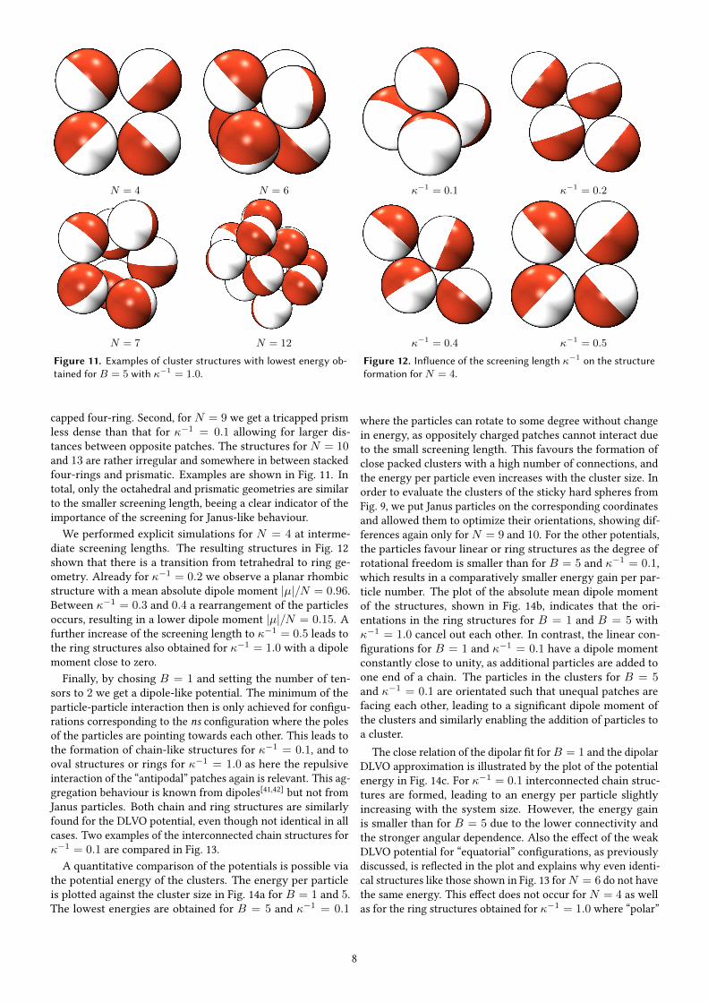
Figure 11. Examples of cluster structures with lowest energy ob-tained for B = 5 with κ−1 = 1.0.
capped four-ring. Second, for N = 9 we get a tricapped prismless dense than that for κ−1 = 0.1 allowing for larger dis-tances between opposite patches. The structures for N = 10and 13 are rather irregular and somewhere in between stackedfour-rings and prismatic. Examples are shown in Fig. 11. Intotal, only the octahedral and prismatic geometries are similarto the smaller screening length, beeing a clear indicator of theimportance of the screening for Janus-like behaviour.
We performed explicit simulations for N = 4 at interme-diate screening lengths. The resulting structures in Fig. 12shown that there is a transition from tetrahedral to ring ge-ometry. Already for κ−1 = 0.2 we observe a planar rhombicstructure with a mean absolute dipole moment |µ|/N = 0.96.Between κ−1 = 0.3 and 0.4 a rearrangement of the particlesoccurs, resulting in a lower dipole moment |µ|/N = 0.15. Afurther increase of the screening length to κ−1 = 0.5 leads tothe ring structures also obtained for κ−1 = 1.0 with a dipolemoment close to zero.
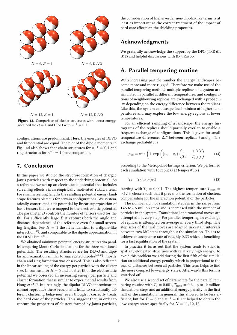
Finally, by chosing B = 1 and setting the number of ten-sors to 2 we get a dipole-like potential. The minimum of theparticle-particle interaction then is only achieved for conVgu-rations corresponding to the ns conVguration where the polesof the particles are pointing towards each other. This leads tothe formation of chain-like structures for κ−1 = 0.1, and tooval structures or rings for κ−1 = 1.0 as here the repulsiveinteraction of the “antipodal” patches again is relevant. This ag-gregation behaviour is known from dipoles[41,42] but not fromJanus particles. Both chain and ring structures are similarlyfound for the DLVO potential, even though not identical in allcases. Two examples of the interconnected chain structures forκ−1 = 0.1 are compared in Fig. 13.
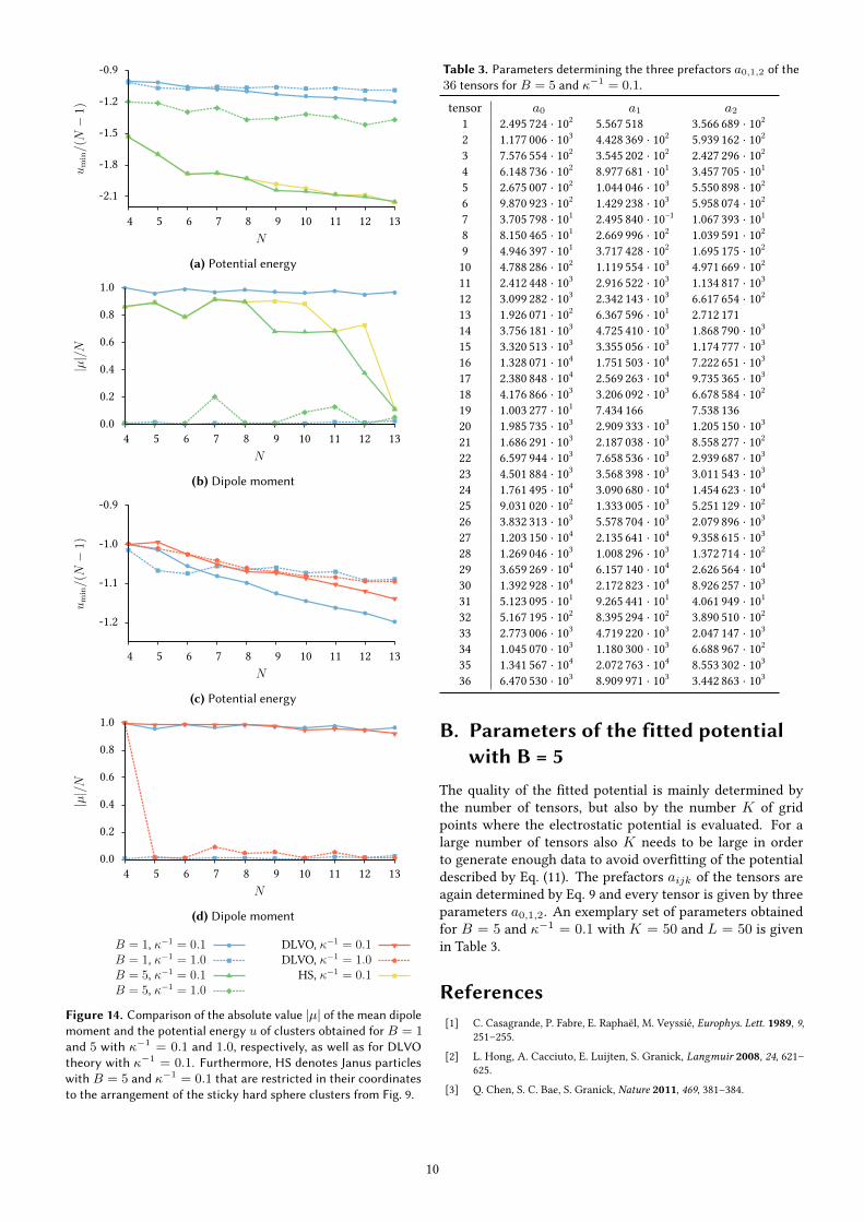
A quantitative comparison of the potentials is possible viathe potential energy of the clusters. The energy per particleis plotted against the cluster size in Fig. 14a for B = 1 and 5.The lowest energies are obtained for B = 5 and κ−1 = 0.1
κ−1 = 0.1 κ−1 = 0.2
κ−1 = 0.4 κ−1 = 0.5
Figure 12. InWuence of the screening length κ−1 on the structureformation for N = 4.
where the particles can rotate to some degree without changein energy, as oppositely charged patches cannot interact dueto the small screening length. This favours the formation ofclose packed clusters with a high number of connections, andthe energy per particle even increases with the cluster size. Inorder to evaluate the clusters of the sticky hard spheres fromFig. 9, we put Janus particles on the corresponding coordinatesand allowed them to optimize their orientations, showing dif-ferences again only for N = 9 and 10. For the other potentials,the particles favour linear or ring structures as the degree ofrotational freedom is smaller than for B = 5 and κ−1 = 0.1,which results in a comparatively smaller energy gain per par-ticle number. The plot of the absolute mean dipole momentof the structures, shown in Fig. 14b, indicates that the ori-entations in the ring structures for B = 1 and B = 5 withκ−1 = 1.0 cancel out each other. In contrast, the linear con-Vgurations for B = 1 and κ−1 = 0.1 have a dipole momentconstantly close to unity, as additional particles are added toone end of a chain. The particles in the clusters for B = 5and κ−1 = 0.1 are orientated such that unequal patches arefacing each other, leading to a signiVcant dipole moment ofthe clusters and similarly enabling the addition of particles toa cluster.
The close relation of the dipolar Vt forB = 1 and the dipolarDLVO approximation is illustrated by the plot of the potentialenergy in Fig. 14c. For κ−1 = 0.1 interconnected chain struc-tures are formed, leading to an energy per particle slightlyincreasing with the system size. However, the energy gainis smaller than for B = 5 due to the lower connectivity andthe stronger angular dependence. Also the eUect of the weakDLVO potential for “equatorial” conVgurations, as previouslydiscussed, is reWected in the plot and explains why even identi-cal structures like those shown in Fig. 13 forN = 6 do not havethe same energy. This eUect does not occur for N = 4 as wellas for the ring structures obtained for κ−1 = 1.0 where “polar”
8
N = 6, B = 1 N = 6, DLVO
N = 12, B = 1 N = 12, DLVO
Figure 13. Comparison of cluster structures with lowest energyobtained for B = 1 and DLVO with κ−1 = 0.1.
conVgurations are predominant. Here, the energies of DLVOand Vt potential are equal. The plot of the dipole moments inFig. 14d also shows that chain structures for κ−1 = 0.1 andring structures for κ−1 = 1.0 are comparable.
7. Conclusion
In this paper we studied the structure formation of chargedJanus particles with respect to the underlying potential. Asa reference we set up an electrostatic potential that includesscreening eUects via an empirically motivated Yukawa term.For small screening lengths the resulting potential energy land-scape features plateaus for certain conVgurations. We system-atically constructed a Vt potential by linear superposition ofbasis tensors that were mapped to the electrostatic potential.The parameter B controls the number of tensors used for theVt. For suXciently large B it captures both the angle anddistance dependence of the reference even for small screen-ing lengths. For B = 1 the Vt is identical to a dipole-likeinteraction[38], and comparable to the dipole approximation inthe DLVO limit[33].
We obtained minimum potential energy structures via paral-lel tempering Monte Carlo simulations for the three mentionedpotentials. The resulting structures are for DLVO and dipo-lar approximation similar to aggregated dipoles[41,42]: mostlychain and ring formation was observed. This is also reWectedin the linear scaling of the energy per particle with the clustersize. In contrast, for B = 5 and a better Vt of the electrostaticpotential we observed an increasing energy per particle andcluster formation that is similar to experimental results fromHong et al.[7]. Interestingly, the dipolar DLVO approximationcannot reproduce these results and leads to structurally dif-ferent clustering behaviour, even though it correctly treatsthe hard core of the particles. This suggest that, in order tocapture the properties of clusters formed by Janus particles,
the consideration of higher-order non-dipolar-like terms is atleast as important as the correct treatment of the impact ofhard core eUects on the shielding properties.
Acknowledgments
We gratefully acknowledge the support by the DFG (TRR 61,B12) and helpful discussions with B.-J. Ravoo.
A. Parallel tempering routine
With increasing particle number the energy landscapes be-come more and more rugged. Therefore we make use of theparallel tempering method: multiple replicas of a system aresimulated in parallel at diUerent temperatures, and conVgura-tions of neighbouring replicas are exchanged with a probabil-ity depending on the energy diUerence between the replicas.Like this, the system can escape local minima at higher tem-peratures and may explore the low energy regions at lowertemperatures.
For an eXcient sampling of a landscape, the energy his-tograms of the replicas should partially overlap to enable afrequent exchange of conVgurations. This is given for smalltemperature diUerences ∆T between replicas i and j. Theexchange probability is
pex = min
(1, exp
((ui − uj)
(1
Ti− 1
Tj
)))(14)
according to the Metropolis-Hastings criterion. We performedeach simulation with 16 replicas at temperatures
Ti = T0 exp (αi) (15)
starting with T0 = 0.001. The highest temperature Tmax =0.12 is chosen such that it prevents the formation of clusters,compensating for the interaction potential of the particles.
The number nsim of simulation steps is in the range from1.65 to 6.5 million steps and is increased with the number ofparticles in the system. Translational and rotational moves areattempted in every step. For parallel tempering an exchangeof replicas is attempted on average in every third step. Thestep sizes of the trial moves are adapted in certain intervalsbetween two MC steps throughout the simulation. This is toachieve an acceptance rate of roughly 0.33 which is beneVtingfor a fast equilibration of the system.
In practice it turns out that the system tends to stick inspatially elongated structures with relatively high energy. Toavoid this problem we add during the Vrst Vfth of the simula-tion an additional energy penalty which is proportional to thesum of distances between all particles. This term helps to Vndthe more compact low-energy states. Afterwards this term isswitched oU.
We also use a second set of parameters for the parallel tem-pering routine with T0 = 0.001, Tmax = 0.3, up to 10 millionsimulations steps and an additional energy penalty in the Vrsthalf of the simulation. In general, this showed to be less ef-Vcient, but for B = 5 and κ−1 = 0.1 it helped to obtain thelow-energy states speciVcally for N = 11, 12, 13.
Figure 14. Comparison of the absolute value |µ| of the mean dipolemoment and the potential energy u of clusters obtained for B = 1and 5 with κ−1 = 0.1 and 1.0, respectively, as well as for DLVOtheory with κ−1 = 0.1. Furthermore, HS denotes Janus particleswith B = 5 and κ−1 = 0.1 that are restricted in their coordinatesto the arrangement of the sticky hard sphere clusters from Fig. 9.
Table 3. Parameters determining the three prefactors a0,1,2 of the36 tensors for B = 5 and κ−1 = 0.1.
The quality of the Vtted potential is mainly determined bythe number of tensors, but also by the number K of gridpoints where the electrostatic potential is evaluated. For alarge number of tensors also K needs to be large in orderto generate enough data to avoid overVtting of the potentialdescribed by Eq. (11). The prefactors aijk of the tensors areagain determined by Eq. 9 and every tensor is given by threeparameters a0,1,2. An exemplary set of parameters obtainedfor B = 5 and κ−1 = 0.1 with K = 50 and L = 50 is givenin Table 3.
References[1] C. Casagrande, P. Fabre, E. Raphaël, M. Veyssié, Europhys. Lett. 1989, 9,
251–255.
[2] L. Hong, A. Cacciuto, E. Luijten, S. Granick, Langmuir 2008, 24, 621–625.
[3] Q. Chen, S. C. Bae, S. Granick, Nature 2011, 469, 381–384.
10
[4] S. K. Smoukov, S. Gangwal, M. Marquez, O. D. Velev, Soft Matter 2009,5, 1285–1292.
[5] S. Sacanna, L. Rossi, D. J. Pine, J. Am. Chem. Soc. 2012, 134, 6112–6115.
[6] J. Yan, M. Bloom, S. C. Bae, E. Luijten, S. Granick, Nature 2012, 491,578–582.
[7] L. Hong, A. Cacciuto, E. Luijten, S. Granick, Nano Letters 2006, 6, 2510–2514.
[8] T. Kaufmann, C. Wendeln, T. Gokmen, S. Rinnen, M. M. Becker, H. F.Arlinghaus, F. du Prez, B. J. Ravoo, Chem. Commun. 2013, 49, 63–65.
[9] W. L. Miller, A. Cacciuto, Phys. Rev. E 2009, 80, 021404.
[10] F. Sciortino, A. Giacometti, G. Pastore, Phys. Chem. Chem. Phys. 2010,12, 11869–11877.
[11] T. Vissers, Z. Preisler, F. Smallenburg, M. Dijkstra, F. Sciortino, J. Chem.Phys. 2013, 138, 164505.